Precise Numerical Solutions of Potential Problems Using Crank-Nicholson Method

Abstract

A new numerical treatment in the Crank-Nicholson method with the imaginary time evolution operator is presented in order to solve the Schrödinger equation. The original time evolution technique is extended to a new operator that provides a systematic way to calculate not only eigenvalues of ground state but also of excited states. This new method systematically produces eigenvalues with accuracies of eleven digits with the Cornell potential that covers non-perturbative regime. An absolute error estimation technique based on a power counting rule is implemented. This method is examined with exactly solvable problems and produces the numerical accuracy down to 10^-11.

Numerical computation of analytically unsolvable Schrödinger equations has been of interest in atomic and molecular physics, quantum chromodynamics, and Bose-Einstein condensation of trapped atomic vapors Mehta ; Vrscay ; Chhajlany ; Chiofalo . Conventionally, a wave function has been represented as a linear combination of plane waves or of atomic orbitals cayley . However, these representations entail high computational cost to calculate the matrix elements for these bases. The plane wave bases set is not suitable for localized orbitals, and the atomic orbital bases set is not suitable for spreading waves. In particular, potential problems such as the Cornell potential Eichten:1978tg ; Eichten:1979ms are difficult to compute precise eigenvalues because they have singularities at the origin and at the infinity, and includes non-perturbative regime when the linear term is significant.

To overcome these problems, numerical methods such as Landé subtraction Norbury and Nystrom plus correction Tang in the momentum space produced eigenvalues with six or seven digits. Others adopted real-space representation Jacobs:1986gv ; Roychoudhury . In these methods, a wave function is discretized by grid points in real space providing from five to seven digits. Also, estimates using the exact solutions of the Killingbeck potential produced eigenvalues with seven digits Chhajlany . Among these real-space methods, a method called Crank-Nicholson (C-N) scheme recipes ; galbrath is known to be especially useful for one-dimensional systems because this method conserves the norm of the wave function exactly and the computation is stable and accurate even in a long time slice. These characteristics are very attractive for solving the Cornell potential in order to compute eigenvalues and eigenstates of the system precisely.

The current numerical precisions in relevant research areas may not be as high as one would hope to achieve. For example, it may forbid one to study fine or hyper-fine structure effects in the atomic system Norbury . Calculation of matrix elements subject to large subtraction may require high accuracy in quantum chromodynamics Bodwin:2006dn ; Bodwin:2006dm . Also, none of the references we compiled for this study contains the serious error estimate on their numerical calculations, which is an important indicator of the reliability of a suggested numerical method.

In this letter, we apply the C-N method to solve the Schrödinger equation and present two new numerical methods. First, the C-N method with the imaginary time evolution operator is re-interpreted by extending its allowed region. This method produces ground-state eigenvalues with numerical accuracies of eleven digits when the Cornell potential is used. We then extend the original time evolution technique to a new operator that provides a systematic way to calculate not only the eigenvalue of the ground state but also those of excited states with less computational time by a factor of 10, while providing the same accuracy as in our re-interpreted C-N method. Our methods will be useful in calculations of eigenstates for the Cornell potential and we discuss some of the results. At the end, we discuss a mathematically simple but rigorous absolute error estimation on the numerical calculations presented in this letter.

C-N method recipes ; galbrath is a finite difference method used for solving diffusive initial-value problems numerically. The main part of this method is the time evolution operation and the evolution operator for the Schrödinger equation may be approximated by Cayley’s form cayley as

$$e^{-i\mathcal{H}t}=\frac{1-\frac{i}{2}\mathcal{H}t}{1+\frac{i}{2}\mathcal{H}t}+\mathcal{O}(\mathcal{H}^{3}t^{3}),$$ (1)

where $\mathcal{H}$ is the Hamiltonian of the problem. This equality is correct up to the second order in $\mathcal{H}t$ and the approximation is valid when $|\mathcal{H}t|$ $\ll$ 1. By multiplying this operator to an initial wave function, one obtains the evolved wave function. The standard C-N method makes use of Eq. (1) in order to study the time evolution of the wave function recipes ; galbrath .

Next, we introduce the imaginary time method Chiofalo to calculate the eigenfunctions and eigenvalues. By a Wick rotation, one replaces $t$ by $-i\tau$ in the time evolution operator Chiofalo . This transforms the original Schrödinger equation into a diffusion equation. Then a wave function evolves in time slice $\Delta t$ as

$$u(\rho,\Delta t)=\sum_{i=1}^{\infty}C_{i}u_{i}(\rho)e^{-i\zeta_{i}\Delta t}=\sum_{i=1}^{\infty}C_{i}u_{i}(\rho)e^{-\zeta_{i}\Delta\tau},$$ (2)

where $u_{i}(\rho)$ and $\zeta_{i}$ are the eigenfunction and the eigenvalue for $i$-th state, respectively. $C_{i}$ is the relative amplitude for $i$-th state and the summation is over all possible eigenstates of the system.

For the imaginary-time version, eigenfunctions decay monotonically in time till the steady state is reached. The ground-state eigenvalue can then be read off from the steady-state eigenfunction as $\tau$ $\rightarrow$ $\infty$ Chiofalo . Therefore, we acknowledge that the time evolution operation itself in the C-N method acts as a tool that selects the ground state only. Here, we advocate that the condition $|\mathcal{H}\tau|\ll$ 1 is not necessary in the calculation of the ground-state eigenvalue. When all the eigenvalues are negative such as the pure Coulomb potential case, where $\zeta_{0}<\cdots<\zeta_{n}<\cdots<0$, the amplification of the ground-state coefficient may happen in the region $-2<\mathcal{H}\tau<0$ as the time evolution continues. On the other hand, when all the eigenvalues are positive such as in problems with the linear and Cornell potentials, where $0<\zeta_{0}<\cdots<\zeta_{n}$, the time evolution operator can amplify the ground-state coefficient in the region $\mathcal{H\tau}<-2$. Note that we relax the condition $|\mathcal{H}\tau|\ll 1$ in order to obtain faster convergence to ground-state eigenfunction even if that region is used in the standard C-N method. We call this approach as a relaxed C-N method.

Once the ground-state wave function is obtained, one can obtain the ground-state eigenvalue from the expectation value of the Hamiltonian of interest. Note that, for the numerical computation of an expectation value, the upper bound of the integral can not be an infinity but a cut-off value, $\rho_{\textrm{max}}$. We will explain how to control the numerical error produced by ignoring the region $(\rho_{\textrm{max}},\infty)$ later.

The spherical Stark effect in hydrogen and a bound state for a heavy quarkonium may be described by the Schrödinger equation with the Cornell potential Eichten:1978tg ; Eichten:1979ms ; Vrscay . The radial part of the Schrödinger equation with orbital-angular-momentum quantum number $\ell$ that is relevant to such problems may be given by

$$\left[-\frac{d^{2}}{d\rho^{2}}+\frac{\ell(\ell+1)}{\rho^{2}}-\frac{\lambda}{\rho}+\rho\right]u(\rho)=\zeta u(\rho),$$ (3)

where the dimensionless wave function $u(\rho)$ and the dimensionless energy eigenvalue $\zeta$ in Eq. (3) are described in Ref. Eichten:1978tg . The parameter $\lambda$ is the relative strength between the Coulomb and the linear potentials. We call it as the coulombic parameter throughout this letter.

The relaxed C-N method is now applied to the Cornell potential problem. The $\lambda$ dependence of the ground-state eigenvalues in Ref. Eichten:1978tg is reproduced with our relaxed C-N method and a comparison of two results is summarized in Table 1. The time evolution in our relaxed C-N method gives eigenvalues over iterations giving stable sixteen-digits and all agree well with the results in Ref. Eichten:1978tg . We also find that the convergence speed is improved by 10 times compared with the standard C-N method that we tested. For excited states, one can in principle obtain the eigenvalues from the lowest to higher states by the Gram-Schmidt orthogonalization procedure. We find that the standard C-N method is not useful in calculating excited states because the convergence speed is practically zero when we require the numerical precision to be 10 digits. However, with the relaxed C-N method, the excited-state eigenvalues are successfully found, with the speed being 10 times slower than the time needed to find the ground state. The amount of time required to calculate excited states is no longer than ten minutes with a Pentium IV CPU with 0.5 GB memory.

$\lambda$	$\zeta$(Ref.Eichten:1978tg )	$\zeta$ (this work)	$\Delta\zeta$
0.0	2.338 107	2.338 107 410 458 750	$1.0\times 10^{-12}$
0.2	2.167 316	2.167 316 208 771 731	$1.0\times 10^{-12}$
0.4	1.988 504	1.988 503 899 749 943	$9.6\times 10^{-13}$
0.6	1.801 074	1.801 073 805 646 145	$8.5\times 10^{-13}$
0.8	1.604 410	1.604 408 543 235 973	$6.6\times 10^{-13}$
1.0	1.397 877	1.397 875 641 659 578	$3.8\times 10^{-13}$
1.2	1.180 836	1.180 833 939 744 863	$2.1\times 10^{-14}$
1.4	0.952 644	0.952 640 495 219 193	$5.8\times 10^{-13}$
1.6	0.712 662	0.712 657 680 462 421	$1.3\times 10^{-12}$
1.8	0.460 266	0.460 260 113 875 977	$2.3\times 10^{-12}$

Table 1: Dependence of the ground-state eigenvalues $\zeta$ on the coulombic parameter $\lambda$. The Cornell potential is used in the calculation. The second column contains the numerical results from Ref. Eichten:1978tg and the third column contains our result with the relaxed C-N method. The number of grid points is set to be $N$ = 300,000 and $\Delta\tau$ = $-$ 5 for the numerical analysis. An estimate on the numerical errors of the computation $\Delta\zeta$ is also listed at the last column and will be discussed later.

We emphasize that the condition $|\mathcal{H}\tau|\ll$ 1 can be relaxed as far as the goal of the numerical computation is to obtain the ground-state eigenfunction. We extend this idea further in order to calculate excited-state eigenvalues and eigenfunctions systematically and more efficiently.

Consider the following operator

$$\frac{1}{\mathcal{H}-\beta},$$ (4)

where $\beta$ is an arbitrary real number in the eigenvalue space. If we apply the operator in Eq. (4) to the wave packet $k$ times,

$$\left(\frac{1}{\mathcal{H}-\beta}\right)^{k}u(\rho)=\sum_{i=1}^{\infty}\frac{C_{i}}{(\zeta_{i}-\beta)^{k}}u_{i}(\rho),$$ (5)

where we assume that the time independent wave packet $u(\rho)$ can be expressed as a linear combination of the infinite number of eigenfunctions $u_{i}(\rho)$ with coefficients $C_{i}$. For $\beta=\zeta_{i}+\epsilon$ such that $|\epsilon|\ll 1$, we have

$$\left|\frac{1}{\zeta_{i}-\beta}\right|\gg\left|\frac{1}{\zeta_{j}-\beta}\right|$$ (6)

if $j\neq i$. Therefore, Eq. (4) plays a role as an amplifier which magnifies the contributions of the term with the nearest eigenvalue from the point $\beta$. In this way, all the eigenvalues within an arbitrary range in $\beta$ can be found systematically, by running $\beta$ within the range. We call this approach as a modified C-N method. Advantages of this method are as follows. First, the calculations of excited states can be carried out systematically by stepping through different values of $\beta$. Second, the computing time for calculating excited-state wave functions or eigenvalues is similar to that needed for the ground state. Furthermore, it does not lose accuracies in the calculation of higher-state eigenvalues while other methods do often. This contrasts the modified C-N method to the relaxed C-N method. With the relaxed C-N method, the Gram-Schumidt orthonormalization slows down the computing speed by ten times, as mentioned before.

First, the modified C-N method is tested on the pure Coulomb potential and to the pure linear potential ($\lambda$ = $0$) where the exact eigenvalues are known for both cases. This is a good benchmark because one directly examines the performance of the algorithm by comparing the exact solutions to the numerical results of the algorithm to be tested. We find that the numerical values of eigenvalues agree well with known analytical values, up to eleven digits. Second, the modified C-N method is applied to the Cornell potential and reproduce the result in Table 1. We find that eleven digits of the eigenvalues are reproduced completely from $\lambda$ = 0.0 to 1.8. This is consistent with our error estimation which will be explained later. Third, the modified C-N method is applied to the calculation of excited states. Table 2 shows the eigenvalues obtained. Note that for the $1S$ state in Table 2, one can compare the eigenvalue with the number in Table 1 and only the last two digits are different, which is again consistent with our error estimation. Again, for the ground state, the relaxed and the modified C-N methods require similar amount of computing time, but for the excited states, the modified C-N method is faster by 10 times. We checked the computing speed for the Coulomb, linear, and Cornell potentials separately and all three give similar performances.

State	$\zeta$	$\Delta\zeta$
$1S$	1.397 875 641 659 581	$3.8\times 10^{-13}$
$2S$	3.475 086 545 392 783	$3.4\times 10^{-12}$
$3S$	5.032 914 359 529 781	$6.3\times 10^{-12}$
$4S$	6.370 149 125 476 954	$9.4\times 10^{-12}$
$5S$	7.574 932 640 578 566	$1.3\times 10^{-11}$
$1P$	2.825 646 640 702 388	$1.2\times 10^{-12}$
$2P$	4.461 863 593 453 813	$3.1\times 10^{-12}$
$3P$	5.847 634 227 299 904	$5.5\times 10^{-12}$
$1D$	3.850 580 006 802 002	$5.9\times 10^{-13}$
$2D$	5.292 984 139 140 243	$2.0\times 10^{-12}$

Table 2: Numerical values of eigenvalues and the error estimation for various excited states with the Cornell potential. The modified C-N method is used to calculate eigenvalues. The coulombic parameter is set to $\lambda=1.0$ and the number of grid points to be $N=300,000$.

There are two sources of errors in our numerical calculation. One is the cut-off ($\rho_{\textrm{max}}$) and the other is the discretization of continuous equations. The cut-off gives the imperfect numerical integration but could in principle be reduced as small as one wishes by increasing the value of $\rho_{\textrm{max}}$. We estimate the error due to the finite value of $\rho_{\textrm{max}}$ for the Coulomb and linear potentials, respectively, by integrating exact eigenfunctions. We find that the error is 10^-15 or smaller when $\rho_{\textrm{max}}$ = 20, for example. In fact, for the practical purpose, we control the value of $\rho_{\textrm{max}}$ in such a way that the numerical error due to finite value of $\rho_{\textrm{max}}$ is smaller than the error from the fact that we deal with discrete processes. This assumes that the error estimates with the Coulomb and linear potentials individually are not significantly different from the errors due to the Cornell potential. Practically, selecting proper values of $\rho_{\textrm{max}}$ is important, because too small values cause large errors and too large values may slow down the computation. We find that $\rho_{\textrm{max}}$ = 30 is an optimal value for most of our applications shown in this letter. Note that $\rho_{\textrm{max}}$ = 30 corresponds to 30 times of the Bohr radius in the hydrogen atom problem, for example.

More serious source of the error is originated from the discretization of continuous differential equations. In this letter, differentiation and integration of wave functions are discretized with the following prescriptions recipes

$$u^{\prime\prime}_{j} = \frac{u_{j+1}-2u_{j}+u_{j-1}}{\Delta\rho^{2}}+\mathcal{O}(\Delta\rho^{2}),$$ (7a)

$$\int d\rho\,u(\rho) = \frac{\Delta\rho}{2}\sum_{j=1}^{N}\left(u_{j+1}+u_{j}\right)+\mathcal{O}(\Delta\rho^{2}),$$ (7b)

where $\Delta\rho$ is the distance between two nearest discrete points in the calculation.

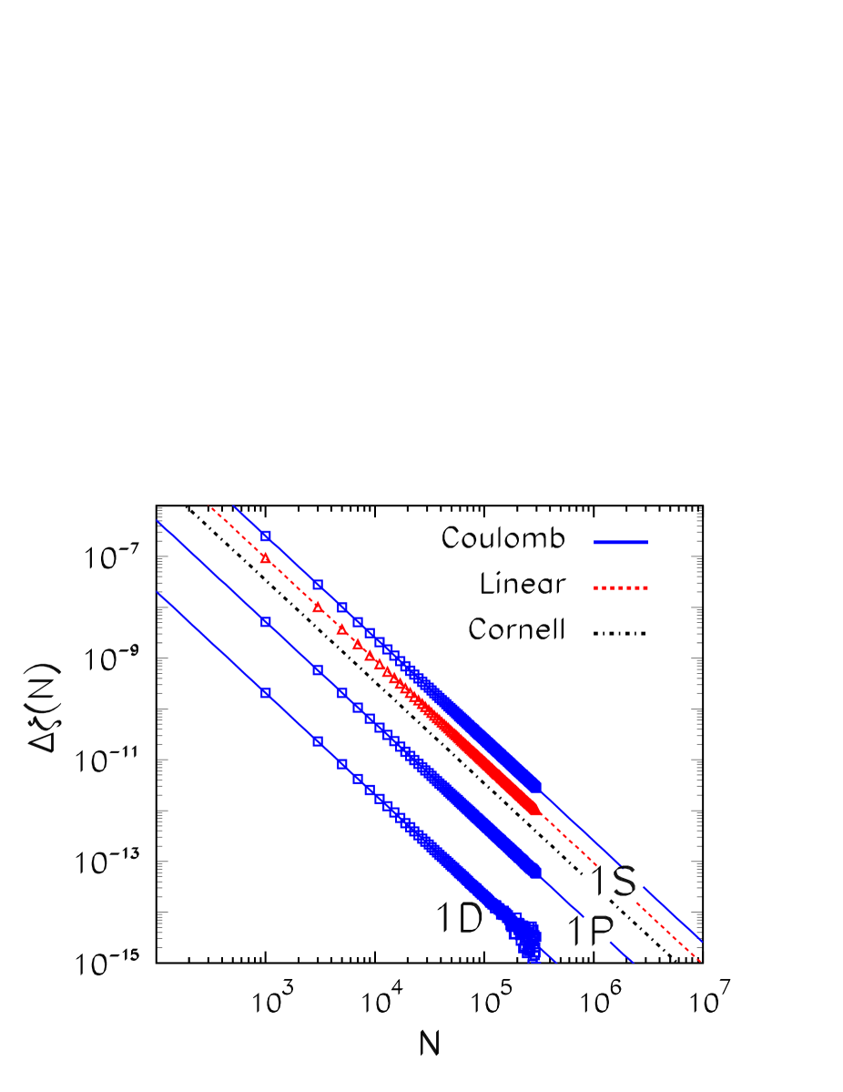
Figure 1: Numerical error estimation for the eigenvalues as a function of the number of grid points. For the Coulomb (linear) potential, $|\zeta_{\textrm{exact}}$ $-$ $\zeta(N)|$ is indicated as open boxes (triangles) for $1S$, $1P$, and $1D$ states ($1S$ state only for the linear potential). The error estimates based on Eq. (8) for the Coulomb, linear, and Cornell potentials are shown in straight, dashed, and dot-dashed lines, respectively. Note that both axes are in logarithmic scales.

From both Eqs. (7a) and (7b), numerical errors contained in the discretization are proportional to $\Delta\rho^{2}=N^{-2}$ where $N$ is the number of grid points in the discretization. Therefore, the error in eigenvalues due to the discretization may be approximated as

$$\Delta\zeta(N)\approx cN^{-2},$$ (8)

where $\Delta\zeta(N)=|\zeta_{\textrm{exact}}-\zeta(N)|$ and the constant $c$ depends on the potential. If we select two arbitrary values in grid points, $N_{1}$ and $N_{2}$, for example, then we can easily obtain the constant $c$ as

$$c\approx\left|\frac{\Delta\zeta(N_{1})-\Delta\zeta(N_{2})}{N_{1}^{-2}-N_{2}^{-2}}\right|=\left|\frac{\zeta(N_{1})-\zeta(N_{2})}{N_{1}^{-2}-N_{2}^{-2}}\right|.$$ (9)

With this, one can estimate the error due to the discretization prescription in Eqs. (7a) and (7b). We refer it as an error estimation from the power counting rule. In Fig. 1, our estimate of the numerical error $\Delta\zeta(N)$ is compared with the true error $|\zeta_{\textrm{exact}}$ $-$ $\zeta(N)|$ for the Coulomb and linear potentials. Here we used our modified C-N method for the error analysis. It is apparent that our error estimate is accurate down to $10^{-11}$ for the $1S$ state under the Coulomb potential, for example, when $N$=300,000. For others, the results are better as in Fig. 1. For the $1D$ state under the Coulomb potential, the true error looks unstable at large value of $N$ and we find that this is due to the limitation in storing significant digits during our computation of $\zeta(N)$. Note that for the Cornell potential, the true errors cannot be calculated because the exact solutions are unknown. Therefore, for the Cornell potential, we estimate that the errors are in the range of $10^{-12}$ as in Fig. 1. We use this error estimation technique throughout this letter and numerical values of the error estimates are included in Tables 1 and 2.

In conclusion, we have presented two numerical methods for calculating Schrödinger equation with the Crank-Nicholson method. In the relaxed C-N method, the time evolution operator is re-interpreted as a weighting operator for finding the ground state eigenfunction more precisely. This idea is extended to a new operator in the modified C-N method that is more efficient in computing not only the ground-state but also excited-state wave functions systematically. An absolute error estimation method is presented based on a power counting rule and is consistent with predictions when exact solutions are known. These two algorithms may be useful when precise numerical results are required. Possible applications may include Cornell potential Eichten:1978tg ; Eichten:1979ms and Bose-Einstein condensation of trapped atomic vapors Chiofalo .

We thank Jungil Lee for his suggestion on this topic and Q-Han Park and Ki-hwan Kim for useful discussion on the numerical treatment. E. W. is indebted to Tai Hyun Yoon for his critical comments on this manuscript. D. K.’s research was supported in part by the Seoul Science Fellowship of Seoul Metropolitan Government and by the Korea Research Foundation Grant funded by the Korean Government (MOEHRD), (KRF-2006-612-C00003). E. W.’s research was supported by grant No. R01-2005-000-10089-0 from the Basic Research Program of the Korea Science & Engineering Foundation.

References

- (1) E. R. Vrscay, Phys. Rev. A 31, 2054 (1985).
- (2) C. H. Mehta and S. H. Datil, Phys. Rev. A 17, 34 (1978).
- (3) S. C. Chhajlany and D. A. Letov, Phys. Rev. A 44, 4725 (1991).
- (4) M. .L. Chiofalo, S. Succi, and M. P. Tosi, Phys. Rev. E 62, 7438 (2000).
- (5) N. Watanabe and M. Tsukada, Phys. Rev. E 62, 2914 (2000).
- (6) E. Eichten, K. Gottfried, T. Kinoshita, K. D. Lane, and T. M. Yan, Phys. Rev. D 17, 3090 (1978); 21, 313(E) (1980).
- (7) E. Eichten, K. Gottfried, T. Kinoshita, K. D. Lane, and T. M. Yan, Phys. Rev. D 21, 203 (1980).
- (8) J. W. Norbury, K. M. Maung, and D. E. Kahana, Phys. Rev. A 50, 2075 (1994).
- (9) A. Tang and J. W. Norbury, Phys. Rev. E 63, 066703 (2001).
- (10) R. Roychoudhury, Y. P. Varshni, and M. Sengupta, Phys. Rev. A 42, 184 (1990).
- (11) S. Jacobs, M. G. Olsson, and C. I. Suchyta, Phys. Rev. D 33, 3338 (1986); 34, 3536(E) (1986).
- (12) W. H. Press, B. P. Flannery, S. A. Teukolsky, and W. T. Vetterling, Numerical Recipes in C: The Art of Scientific Computing, (Cambridge University Press, 1992).
- (13) I. Galbraith, Y. S. Ching, and E. Abraham, Am. J. Phys. 52, 60 (1984).
- (14) G. T. Bodwin, D. Kang, and J. Lee, Phys. Rev. D 74, 014014 (2006) [arXiv:hep-ph/0603186].
- (15) G. T. Bodwin, D. Kang, and J. Lee, arXiv:hep-ph/0603185.