Phase sensitive detection of dipole radiation in a fiber-based high numerical aperture optical system

Abstract

We theoretically study the problem of detecting dipole radiation in an optical system of high numerical aperture in which the detector is sensitive to field amplitude. In particular, we model the phase sensitive detector as a single-mode cylindrical optical fiber. We find that the maximum in collection efficiency of the dipole radiation does not coincide with the optimum resolution for the light gathering instrument. The calculated results are important for analyzing fiber-based confocal microscope performance in fluorescence and spectroscopic studies of single molecules and/or quantum dots.

The confocal microscope is a ubiquitous tool for the optical study and characterization of single nanoscale objects. The rejection of stray light from the optical detector afforded by the confocal microscope, combined with its three-dimensional resolution, makes it an ideal instrument for studying physical systems with weak light emission properties novotnyhecht ; inoue . The electromagnetic dipole is the canonical choice for modeling the radiative properties of most physical systems. And, although the vector-field image of an electromagnetic dipole in a high numerical aperture confocal microscope has been known for some time sheppard2 , only recently have the light gathering properties of the instrument been studied. Specifically, the collection efficiency function for a confocal microscope based on a hard-stop aperture was defined and studied by Enderlein enderlein . Such a confocal microscope is sensitive to field intensity and the detected optical power is obtained by integrating the component of the dipole image field Poynting vector that is perpendicular to the hard-stop aperture over the aperture area.

Confocal microscopes based instead on optical fiber apertures have also been investigated. The image forming properties of both coherentgu1 and incoherentgan1 fiber-based confocal microscopes, as well as the light gathering propertiesgu2 of the microscope with a reflecting object have all been examined assuming the paraxial approximation to scalar diffraction theory. Since high numerical aperture fiber-based confocal microscopes are routinely employed in the study of silicon integrated circuits ippolito2 , single semiconductor quantum dots liu2 and other nanoscale light emitters, it is of great practical interest to understand the light collection properties of the fiber-based instrument. Here, we will extend the previous studies by using the angular spectrum representation (ASR)wolf ; richards ; novotnyhecht to study the coupling of dipole radiation into a single-mode optical fiber confocal .

For the calculation below, we assume the optical system illustrated in Fig. 1 is aplanatic. In what follows, we refer to reference sphere 1 as the collection objective and reference sphere 2 as the focusing objective. Initially, we assume the dipole $\vec{\mathbf{d}}$ is placed at the Gaussian focus of the collection objective. The cylindrical optical fiber facet is assumed to be positioned such that it is coaxial with the optical system axis (in Fig. 1) and its flat face is parallel with the focal plane of the focusing objective. We define the relevant angles and unit vectors in Fig. 1 as follows:

$$\begin{array}[]{c}\hat{\mathbf{n}}_{\phi_{1}}=-\hat{\mathbf{n}}_{\phi_{3}}=-\sin{\phi_{1}}\hat{\mathbf{n}}_{x}+\cos{\phi_{1}}\hat{\mathbf{n}}_{y}\\ \hat{\mathbf{n}}_{\theta_{1}}=-\hat{\mathbf{n}}_{\theta_{3}}=\cos{\theta_{1}}\cos{\phi_{1}}\hat{\mathbf{n}}_{x}+\cos{\theta_{1}}\sin{\phi_{1}}\hat{\mathbf{n}}_{y}-\sin{\theta_{1}}\hat{\mathbf{n}}_{z}\end{array}$$ (1)

where we define the spherical coordinates $(\theta_{1},\phi_{1})$ ($(\theta_{3},\phi_{3})$) in the object space (image space) to describe the orientation of the wavevector $\vec{\mathbf{k}}_{1}$ ($\vec{\mathbf{k}}_{3}$), and ensure that in each section of the optical system all coordinate systems are right-handed. In addition, the sine condition relates the polar angles in the object and image space as $f_{1}\sin{\theta_{1}}=f_{3}\sin{\theta_{3}}$ where we have introduced the focal length $f_{1}$ ($f_{3}$) for the collection (focusing) objective. The geometry implies the azimuthal angles are related according to $\phi_{1}=\phi_{3}-\pi$.

To calculate the vector-wave-optics image of the dipole, we employ the ASR and express the image dipole field as

$$\vec{\mathbf{E}}_{3}(\rho_{3},\varphi_{3},z_{3})=\frac{\omega^{2}}{\epsilon_{o}c^{2}}\frac{i\tilde{M}k_{3}e^{if_{1}(k_{1}-k_{3}\tilde{M})}}{8\pi^{2}}\int_{0}^{\theta^{max}_{3}}\int_{0}^{2\pi}d\theta_{3}\,d\phi_{3}\,\sqrt{\frac{n_{1}\cos\theta_{3}}{n_{3}\cos\theta_{1}}}\sin\theta_{3}$$

$$\times\biggl{\{}-\hat{\mathbf{n}}_{\theta_{3}}[\hat{\mathbf{n}}_{\theta_{3}}\cdot\vec{\mathbf{E}}_{d}(\theta_{3},\phi_{3})]-\hat{\mathbf{n}}_{\phi_{3}}[\hat{\mathbf{n}}_{\phi_{3}}\cdot\vec{\mathbf{E}}_{d}(\theta_{3},\phi_{3})]\biggr{\}}e^{ik_{3}(\rho_{3}\sin\theta_{3}\cos(\phi_{3}-\varphi_{3})+z_{3}\cos\theta_{3})}$$ (2)

where we have defined the focal length ratio $\tilde{M}=(f_{3}/f_{1})$ (the magnification $M$ of the optical system relates to $\tilde{M}$ as $M=\tilde{M}n_{1}/n_{3}$), the magnitude of the wavevectors $k_{i}=|\vec{\mathbf{k}}_{i}|$, and integrate over the polar angle $\theta_{3}$ and the azimuthal angle $\phi_{3}$ in the image space. To arrive at Eq. (Phase sensitive detection of dipole radiation in a fiber-based high numerical aperture optical system), we map the vector electric far field of the dipole across the collection objective and then across the focusing objective according to the unit vector mappings defined in Fig. 1. We find it convenient to integrate over the object space polar angle. Introducing the identity $d\theta_{3}\sin\theta_{3}=(\sin\theta_{1}\cos\theta_{1}/\tilde{M}^{2}\cos\theta_{3})d\theta_{1}$ into Eq. (Phase sensitive detection of dipole radiation in a fiber-based high numerical aperture optical system) and using Bessel function identities novotnyhecht to integrate over the azimuthal angle $\phi_{3}$ we find Sign

$$\vec{\mathbf{E}}^{x}_{3}(\rho_{3},\varphi_{3},z_{3})=C(f_{1},f_{3})d_{x}\left[\begin{array}[]{c}\tilde{I}_{d0}(\rho_{3},z_{3})+\tilde{I}_{d2}(\rho_{3},z_{3})\cos 2\varphi_{3}\\ \tilde{I}_{d2}(\rho_{3},z_{3})\sin 2\varphi_{3}\\ -2i\tilde{I}_{d1,2}(\rho_{3},z_{3})\cos\varphi_{3}\end{array}\right],$$ (6)

$$\vec{\mathbf{E}}^{y}_{3}(\rho_{3},\varphi_{3},z_{3})=C(f_{1},f_{3})d_{y}\left[\begin{array}[]{c}\tilde{I}_{d2}(\rho_{3},z_{3})\sin 2\varphi_{3}\\ \tilde{I}_{d0}(\rho_{3},z_{3})-\tilde{I}_{d2}(\rho_{3},z_{3})\cos 2\varphi_{3}\\ -2i\tilde{I}_{d1,2}(\rho_{3},z_{3})\sin\varphi_{3}\end{array}\right],$$ (10)

and

$$\vec{\mathbf{E}}^{z}_{3}(\rho_{3},\varphi_{3},z_{3})=C(f_{1},f_{3})d_{z}\left[\begin{array}[]{c}2i\tilde{I}_{d1}(\rho_{3},z_{3})\cos\varphi_{3}\\ 2i\tilde{I}_{d1}(\rho_{3},z_{3})\sin\varphi_{3}\\ -2\tilde{I}_{d0,2}(\rho_{3},z_{3})\end{array}\right]$$ (14)

where

$$C(f_{1},f_{3})=\frac{\omega^{2}}{\epsilon_{o}c^{2}}\frac{ik_{3}e^{if_{1}(k_{1}-k_{3}\tilde{M})}}{8\pi\tilde{M}}\sqrt{\frac{n_{1}}{n_{3}}}$$ (15)

and we use the notation $\vec{\mathbf{E}}^{j}_{3}(\rho_{3},\varphi_{3},z_{3})$ for the image field of a $j$-oriented dipole in the object space expressed in terms of Cartesian unit vectors. The integrals $\tilde{I}_{dn}(\rho_{3},z_{3})$ are defined as

$$\begin{array}[]{c}\tilde{I}_{d0}(\rho_{3},z_{3})=\int_{0}^{\theta^{max}_{1}}d\theta_{1}e^{ik_{3}z_{3}g(\theta_{1})}\sqrt{\frac{\cos\theta_{1}}{g(\theta_{1})}}\sin\theta_{1}\biggr{(}1+\cos\theta_{1}g(\theta_{1})\biggl{)}J_{0}\,,\\ \\ \tilde{I}_{d1}(\rho_{3},z_{3})=\int_{0}^{\theta^{max}_{1}}d\theta_{1}e^{ik_{3}z_{3}g(\theta_{1})}\sqrt{\cos\theta_{1}}\sin^{2}\theta_{1}J_{1}\,,\\ \\ \tilde{I}_{d2}(\rho_{3},z_{3})=\int_{0}^{\theta^{max}_{1}}d\theta_{1}e^{ik_{3}zg(\theta_{1})}\sqrt{\frac{\cos\theta_{1}}{g(\theta_{1})}}\sin\theta_{1}\biggr{(}1-\cos\theta_{1}g(\theta_{1})\biggl{)}J_{2}\,,\\ \\ \tilde{I}_{d0,2}(\rho_{3},z_{3})=\int_{0}^{\theta^{max}_{1}}d\theta_{1}e^{ik_{3}z_{3}g(\theta_{1})}\sqrt{\frac{\cos\theta_{1}}{g(\theta_{1})}}\frac{\sin^{3}\theta_{1}}{\tilde{M}^{2}}J_{0}\,,\end{array}$$ (17)

and

$$\begin{array}[]{c}\tilde{I}_{d1,2}(\rho_{3},z_{3})=\int_{0}^{\theta^{max}_{1}}d\theta_{1}e^{ik_{3}z_{3}g(\theta_{1})}\sqrt{\frac{\cos\theta_{1}}{g(\theta_{1})}}\frac{\cos\theta_{1}\sin^{2}\theta_{1}}{\tilde{M}^{2}}J_{1}\end{array}$$ (19)

where $g(\theta_{1})=\sqrt{1-(\sin\theta_{1}/\tilde{M})^{2}}$, the numerical aperture ($NA_{1}$) in the object space defines $\theta^{max}_{1}$ as $NA_{1}=n_{1}\sin\theta^{max}_{1}$ and $J_{m}$ are order $m=0,1,2$ ordinary Bessel functions with argument $(k_{3}\rho_{3}/\tilde{M})\sin\theta_{1}$. Equations (14) - (19) assume the dipole is situated at the Gaussian focus of the collection objective. To express the image of a displaced dipole located at $(\rho_{o},\phi_{o},z_{o}$), we use the imaging property of the optical system and introduce $\rho_{new}=\rho_{3}+M\rho_{o}$, $\varphi_{3}=\varphi_{o}$ and $z_{new}=z_{3}+z_{o}M^{2}(n_{3}/n_{1})$ into Eqs. (14) - (19) where $M$ is the optical system magnification.

We model the case when the phase sensitive detector of the dipole field is a single-mode cylindrical optical fiber situated in the image space of the optical system. We define the collection efficiency $\eta(\vec{\mathbf{r}}_{o},\vec{\mathbf{d}};\tilde{M})$ of the optical fiber as

$$\eta(\vec{\mathbf{r}}_{o},\vec{\mathbf{d}};\tilde{M})=\frac{|\int\int\vec{\mathbf{E}}^{\ast}_{3}(\vec{\mathbf{r}}_{3};\vec{\mathbf{r}}_{o},\vec{\mathbf{d}})\cdot\vec{\mathbf{E}}^{j}_{lm}(\vec{\mathbf{r}}_{3})\,dA_{3}|^{2}}{\int\int|\vec{\mathbf{E}}_{3}(\vec{\mathbf{r}}_{3};\vec{\mathbf{r}}_{o}=0,\vec{\mathbf{d}})|^{2}\,dA_{3}\int\int|\vec{\mathbf{E}}^{j}_{lm}(\vec{\mathbf{r}}_{3})|^{2}\,dA_{3}}$$ (20)

where we make explicit the dependence of $\eta(\vec{\mathbf{r}}_{o},\vec{\mathbf{d}};\tilde{M})$ on the dipole location $\vec{\mathbf{r}}_{o}$ and orientation $\vec{\mathbf{d}}$ in the object space, and on the objective focal length ratio $\tilde{M}$ of the optical system illustrated in Fig. 1 (we condense notation by introducing $\vec{\mathbf{r}}_{3}=(\rho_{3},\varphi_{3},z_{3})$). We point out the collection efficiency, as defined in Eq. (20), depends on the overlap of the dipole image field amplitude with the fiber mode profile and not on the intensity of the dipole image field. For the single-mode optical fiber we make the weakly guiding approximationgloge and assume the cladding refractive index, $n_{cl}$, is nearly equal to the core refractive index, $n_{co}$. The utility of the weakly guiding approximation is that the propagating mode solutions for the fiber, $\vec{\mathbf{E}}^{j}_{lm}(\vec{\mathbf{r}}_{3})$, are linearly polarized (along the direction indexed by $j$). For each propagating solution, characterized by propagation constant $\beta$, there exist two orthogonal, linearly polarized modes typically referred to as the $\mathbf{LP}_{lm}$ modes. Specifically, for a fiber with core radius $a$, the single-mode fiber electric field solutions arebuck

$$\vec{\mathbf{E}}^{x}_{01}(\vec{\mathbf{r}},t)=\left\{\begin{array}[]{c c}\sqrt{\frac{2Z}{\pi a^{2}}\frac{1}{\frac{J^{2}_{1}(u)V^{2}}{w^{2}}}}J_{0}(\frac{ur}{a})e^{i\beta z}\,\mathbf{\hat{n}}_{x}&r\leq a\\ \sqrt{\frac{2Z}{\pi a^{2}}\frac{1}{\frac{J^{2}_{1}(u)V^{2}}{w^{2}}}}\frac{J_{0}(u)}{K_{0}(w)}K_{0}(\frac{wr}{a})e^{i\beta z}\,\mathbf{\hat{n}}_{x}&r\geq a\\ \end{array}\right.$$ (23)

where $u=a\sqrt{n^{2}_{co}k^{2}_{o}-\beta^{2}}$ and $w=a\sqrt{\beta^{2}-n^{2}_{cl}k^{2}_{o}}$ are the transverse wavenumbers in the fiber core and cladding, $V^{2}=u^{2}+w^{2}=ak_{o}\sqrt{n^{2}_{co}-n^{2}_{cl}}$ is the fiber $V$-parameter, $K_{l}$ is the order $l$ modified Bessel function of the second kind, $Z$ is the characteristic impedance of the fiber core and the solution for the orthogonally polarized solution is obtained by interchanging $x$ with $y$ in Eq. (23).

Next, we apply the previous formalism to study the collection efficiency of a fiber-based confocal microscope. First, we position the dipole in a region of refractive index $n_{1}=1.33$ at the focus (equal to the coordinate origin) of a $NA_{1}=1.2\,$ collection objective and calculate the collection efficiency $\eta(\vec{\mathbf{r}}_{o}=0;\tilde{M})$, averaged over a uniform distribution of dipole orientations in the object space, as a function of $\tilde{M}$. In addition, the single-mode fiber core radius is fixed to $0.5\lambda$ ($\lambda$ is the wavelength of the dipole radiation) and the fiber $V$-parameter is equal to 1.03. For the case of the two linearly polarized fiber modes, the collection efficiency is expressible as an incoherent sum of the contribution from each fiber polarization mode $\eta=\eta^{x}+\eta^{y}$ (we assume the modes are linearly polarized along the $x$ and $y$ directions). The result is the solid black line decorated with squares plotted in Fig. 2(a), showing that the maximum collection efficiency is obtained when the ratio of the two objective focal lengths $\tilde{M}=f_{1}/f_{3}=7$ (corresponding to an optical system magnification of $M=9.31$). At this focal length ratio, we calculate a coupling efficiency of approximately fifty-one percent. From our definition of Eq. (20), fifty-one percent of the dipole radiation that enters the microscope image space is coupled into the single-mode optical fiber.

Fixing the magnification to $M=9.31$, and keeping $NA_{1}$ of the collection objective equal to 1.2, we calculate collection efficiency $\eta(\rho_{o}=x,\phi_{o}=0,z_{o}=z;\tilde{M}=7)$ when the dipole is displaced in the object space. The results are presented in Fig. 2(b). The inset of Fig. 2(b) displays linecuts along $x$ $(z_{o}=0)$ and $z$ $(x_{o}=0)$. We find a full width at half maximum (FWHM) of approximately $0.522\lambda$ along the $x$-direction and approximately $2.92\lambda$ along the axis of the microscope. The product of these numbers provides us with a rough estimate of the dipole radiation collection volume (three-dimensional optical resolution) for this fiber-based confocal microscope. In this case the number is approximately $0.795\lambda^{3}$. We also studied the transverse resolution (along the $x$-direction) of the optical system by calculating the FWHM as the focal length ratio was varied around the value that resulted in maximum collection efficiency. The solid black line in Fig. 2(a) is the result of the calculation. We find that the minimum of the FWHM (the optimal resolution) does not coincide with the maximum of collection efficiency. At the focal length ratio $\tilde{M}$ that maximizes the collection efficiency the transverse resolution is approximately nine percent larger than the optimal transverse resolution. Finally, for comparison, the solid vertical line in Fig. 2(a) is both the collection efficiency and transverse resolution when $\tilde{M}=NA_{1}/(n_{1}NA_{3})$ where $NA_{3}=0.13$ for the assumed single-mode fiber. By choosing the focal length ratio to match the refractive index-scaled numerical aperture ratio, the ability of the resulting optical system to collect radiation from the dipole is maximized.

In summary, for a set of fixed optical system constraints, we find that there is a particular value of another system parameter that optimizes the overlap of the conjugated dipole image field amplitude with the fiber mode profile and maximizes the collection efficiency as defined in Eq. (20). In the example here, for fixed collection objective numerical aperture and single-mode fiber characteristics, there is a particular value of the objective focal length ratio $\tilde{M}$ that maximizes the collection efficiency $\eta$. However, Fig. 2(a) makes clear that in constructing a fiber-based confocal microscope there is a compromise between instrument collection efficiency and optical resolution. It is important in system design to determine which figure of merit, collection efficiency or resolution, is most important.

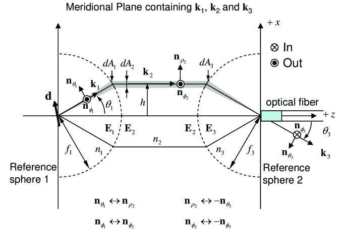
Figure 1: The optical system geometry used to image an arbitrarily oriented dipole $\vec{\mathbf{d}}$. The phase sensitive detector, an optical fiber, is situated in the image space of the microscope.

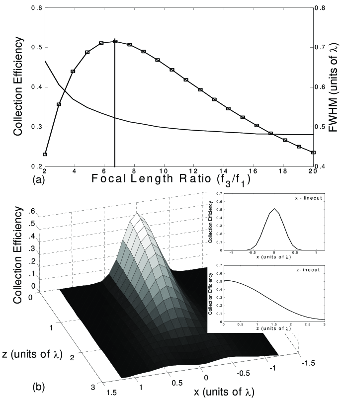
Figure 2: (a) The collection efficiency defined in Eq. (20) and the full width at half maximum (FWHM) of the linecut $\eta(x_{o}=x,z_{o}=0)$ as a function of $\tilde{M}=f_{3}/f_{1}$. The curves make apparent the compromise between collection efficiency and optical resolution. The solid vertical line is the collection efficiency and FWHM for $\tilde{M}=NA_{1}/(n_{1}NA_{3})$ where we use $NA_{3}=0.13$ for the assumed single mode fiber. (b) The collection efficiency defined in Eq. (20) as the dipole is displaced in the object space of the microscope fixing $M=9.31$. The inset of (b) shows linecuts along $(x_{o}=x,z_{o}=0)$ and $(x_{o}=0,z_{o}=z)$. For both (a) and (b) $n_{1}=1.33$, $n_{3}=1$, $a=0.5\lambda$, $V=1.03$, and the collection objective $NA_{1}=1.2$.

References

(1)
L. Novotny and B. Hecht, Principles of Nano-Optics, 1st ed., (Cambridge University
Press, 2006).
(2)
S. Inuoue, in Handbook of Biological Confocal Microscopy, 2nd ed., J. B.
Pawley, ed. (Plenum, New York, 1995), p. 1.
(3)
C.J.R. Sheppard, and T. Wilson, Proc. Roy. Soc. London Ser. A 379, 145
(1982).
(4)
J. Enderlein, Opt. Lett. 25, 634 (2000).
(5)
M. Gu, C.J.R. Sheppard, and X. Gan, J. Opt. Soc. Am. A 8, 1755 (1991).
(6)
X. Gan, M. Gu, and C.J.R. Sheppard, J. Mod. Opt. 39, 825 (1992).
(7)
M. Gu, and C.J.R. Sheppard, J. Mod. Opt. 38, 1621 (1991).
(8)
S.B. Ippolito, B.B. Goldberg, and M.S. Ünlü, J. Appl. Phys. 97,
053105 (2005).
(9)
Z. Liu, B. B. Goldberg, S. B. Ippolito, A. N. Vamivakas, M. S. Ünlü,
and R. P. Mirin, Appl. Phys. Lett. 87, 071905 (2005).
(10)
E. Wolf, Proc. Roy. Soc. London A 253, 349 (1959).
(11)
B. Richards and E. Wolf, Proc. Roy. Soc. London A 253, 358 (1959).
(12)
In our analysis we assume a point emitter and point detector so we refer to the
optical system as a confocal microscope. However, our results can be applied
to other optical systems since there is no assumption on the mechanism for
dipole excitation.
(13)
Our results for the image of the dipole differ from those of Novotny and Hecht novotnyhecht
by a minus sign for the x and y field components of an x-oriented and
y-oriented dipole. The sign difference does not effect physically
important quantities such as energy, power flux or intensity.
(14)
D. Gloge, Appl. Opt. 10, 2252 (1971).
(15)
J. Buck, Fundamentals of Optical Fibers, Ed., (John Wiley and
Sons, New Jersey, 2004).