Optical Feshbach resonances of Alkaline-Earth atoms in a 1D or 2D optical lattice

Abstract

Motivated by a recent experiment by Zelevinsky et al. [Phys. Rev. Lett. 96, 203201], we present the theory for photoassociation and optical Feshbach resonances of atoms confined in a tight one-dimensional (1D) or two-dimensional (2D) optical lattice. In the case of an alkaline-earth intercombination resonance, the narrow natural width of the line makes it possible to observe clear manifestations of the dimensionality, as well as some sensitivity to the scattering length of the atoms. Among possible applications, a 2D lattice may be used to increase the spectroscopic resolution by about one order of magnitude. Furthermore, a 1D lattice induces a shift which provides a new way of determining the strength of a resonance by spectroscopic measurements.

I Introduction

There is a growing experimental effort to study the properties of ultracold alkaline-earth vapours. One of the reasons is that the narrow intercombination resonance of alkaline-earth species (weakly coupling $\,{}^{1}S_{0}$ and $\,{}^{3}P_{1}$ states) can be used to build optical atomic clocks which could be more accurate than the current atomic standard of time Katori et al. (2003); Ido et al. (2005); Ludlow et al. (2006). The Bose-condensation of Ytterbium Takasu et al. (2003), whose atomic structure is close to alkaline-earth species, has also raised the hope of condensing these species. To reach these goals, a good knowledge, and possibly control, of alkaline-earth atomic interactions are needed. Photoassociation, the process of associating pairs of colliding atoms into excited bound states by making them absorb a resonant photon, appears as the best tool to characterize and control these interactions. Indeed, photoassociation can be used as a spectroscopic tool to measure energy levels in excited molecular states Nagel et al. (2005); Takasu et al. (2004); Tojo et al. (2006) and characterize ground-state atomic interactions Mickelson et al. (2005). It can also be regarded as an optical Feshbach resonance Fedichev et al. (1996), analogous to magnetic Feshbach resonances in alkali systems, making it possible to alter these interactions Ciurylo et al. (2005). This is particularly useful for alkaline-earth systems with no hyperfine structure, where magnetic Feshbach resonance is not possible.

Photoassociation near the intercombination resonance is characterized by narrow lines which are sensitive to effects like recoil shifts (due to the momentum of the absorbed photon) and Doppler broadening. These effects can be eliminated by strongly confining the atoms in the direction of propagation of the photoassociation light. This has been demonstrated by trapping the atoms in tight optical lattices Ido and Katori (2003); Takamoto and Katori (2003); Ludlow et al. (2006); Zelevinsky et al. (2006). The wave length of the lattice can be adjusted to its “magic” value Ido and Katori (2003), so that atoms in the ground state and the excited state feel the same trapping potential.

In turn, it is known that strong confinement may affect the collisional properties of the atoms Olshanii (1998); Petrov and Shlyapnikov (2001). We can therefore expect photoassociation to be different in an optical lattice than it is in free space. The purpose of this paper is to investigate how photoassociation spectroscopy and optical Feshbach resonances are affected by a one-dimensional (1D) or two-dimensional (2D) optical lattice. In Section II, we present the general theory of resonant collisions in a 1D and 2D optical lattice, building upon the works of D. S. Petrov and G. V. Shlyapnikov Petrov and Shlyapnikov (2001) and M. Olshanii Olshanii (1998). In section III, we apply the theory to the case of alkaline-earth species. In section IV, we conclude on the possible effects and uses of alkaline-earth photoassociation in optical lattices.

II Optical resonances in a 1d or 2D lattice

An optical lattice is obtained using a standing wave laser which creates a sinusoidal periodic trap. Each cell of this lattice confines the atoms in either a pancake-shaped cloud (for 1D lattices) or cigar-shaped cloud (for 2D lattices). For this reason, we will refer to 1D lattices as a 2D (pancake) geometry, and to 2D lattices as 1D (cigar) geometry. We will assume that there is little transfer between each cloud, so that we can treat each one independently. The atoms in each cloud will be assumed free to move in the directions which are not confined by the lattice, ie, the transverse directions $x,y$ for a 1D lattice, and the axial direction $z$ for a 2D lattice. We will also describe the confinement induced by the lattice near the centre of each cell by a harmonic potential, which is valid if the lattice is tight or strong enough.

To describe optical resonances under such confinement, we use the theories of collisions in 1D or 2D geometries of Refs. Olshanii (1998); Petrov and Shlyapnikov (2001). We express these theories in paragraph II.1 in terms of an energy-dependent scattering length $a(k)$, which is essentially the $K$-matrix for 3D collisions. The original theories were formulated in terms of the usual (energy-independent) scattering length, but taking into account the energy-dependence extends the range of validity of the theories Naidon et al. (2006), and is necessary in the case of resonant collisions. We then give the expression for $a(k)$ in the case of resonant collision in paragraph II.2. Using this expression, we deduce the collisional and photoassociation rates in 1D and 2D geometries.

Similar methods have been used to treat specific cases: a $K$-matrix approach was used in Ref. Wouters et al. (2003) to describe bosonic resonant collisions in a 2D geometry, a multi-channel $K$-matrix approach was used in Ref. Granger and Blume (2004) to describe collisions of spin-polarized fermions in a 1D geometry, and a renormalization approach was used in Refs. Yurovsky (2005, 2006) to describe resonant collisions of bosons in a 1D geometry. All these works relate the effective 1D or 2D scattering properties to the free-space properties. Also closely related are the constructions of pseudo-potentials which can treat confined systems Bolda et al. (2003); Kanjilal and Blume (2004); Stock et al. (2005) and pseudo-potentials in low-dimensional systems Kanjilal and Blume (2004, 2006).

II.1 Collisions in a 1D or 2D confined geometry

Let us briefly review here the method of Refs. Olshanii (1998); Petrov and Shlyapnikov (2001). The stationary states $\psi(\mathbf{r})$ for the relative motion of two atoms confined by a harmonic potential $V(r)$ are given by the Schrödinger equation

$$\left[-\frac{\hbar^{2}}{2\mu}\nabla_{\vec{r}}^{2}+U(r)+V(\vec{r})\right]\psi(\vec{r})=E\psi(\vec{r})$$ (1)

where $\vec{r}=(x,y,z)$ is the relative coordinate between the two atoms with length $r=|\vec{r}|$, $\mu$ is their reduced mass, $U(r)$ is their interaction potential, $E$ is their relative motion energy. In a 2D geometry (1D confinement) the trapping potential is:

$$V(\vec{r})\equiv V_{2D}(\vec{r})=\frac{1}{2}\mu\Omega^{2}z^{2}$$

where $\Omega$ is the frequency of the trap. In a 1D geometry (2D confinement), it is:

$$V(\vec{r})\equiv V_{1D}(\vec{r})=\frac{1}{2}\mu\Omega^{2}\vec{\rho}^{\,2}$$

with $\vec{\rho}=(x,y)$.

At separation $r$ larger than the range $r_{0}$ of the interaction potential $U$, the stationary states can be written as a linear combination of products of a harmonic oscillator eigenstate in the confined direction and a free wave in the weak direction. We choose the conventional basis where each stationary state in the weak direction is asymptotically the sum of an incident plane wave and a scattered wave (which is assumed isotropic for low energies). In 2D and 1D, we have respectively:

$$\psi_{\nu,\vec{q}}^{2D}(\vec{r})\xrightarrow[r>r_{0}]{}\varphi_{\nu}(z)e^{i\vec{q}\cdot\vec{\rho}}+\sum_{\nu}f_{\nu,\nu^{\prime}}^{E}\varphi_{\nu^{\prime}}(z)\sqrt{\frac{i}{8\pi q^{\prime}\rho}}e^{iq^{\prime}\rho}$$ (2)

$$\psi_{n,m,p}^{1D}(\vec{r})\mathop{\to}_{r>r_{0}}\phi_{nm}(\rho)e^{ipz}+\sum_{n^{\prime}m^{\prime}}f_{nm,n^{\prime}m^{\prime}}^{E}\phi_{n^{\prime}m^{\prime}}(\rho)e^{ip^{\prime}|z|}$$ (3)

where $\varphi_{\nu}$, $\phi_{nm}$ are respectively the unit-normalized 1D (2D) harmonic oscillator wave function of vibration index $\nu$ (principal number $n$ and angular momentum number $m$), $p$ is the wave number of the incoming 1D wave, and $\vec{q}$ is the wave vector of the incoming 2D plane wave with wave number $q$. For each state, the total energy $E$ is composed of the oscillator energy in the confined direction, and the free particle energy in the weak direction:

$$E_{2D} = \begin{array}[]{c}\hbar\Omega(\frac{1}{2}+\nu)\end{array}+\frac{\hbar^{2}\vec{q}^{\,2}}{2\mu}$$ (5)

$$= \begin{array}[]{c}\hbar\Omega(\frac{1}{2}+\nu^{\prime})\end{array}+\frac{\hbar^{2}q^{\prime 2}}{2\mu}$$ (7)

$$E_{1D} = \begin{array}[]{c}\hbar\Omega(1+2n+|m|)\end{array}+\frac{\hbar^{2}p^{2}}{2\mu}$$ (9)

$$= \begin{array}[]{c}\hbar\Omega(1+2n^{\prime}+|m^{\prime}|)\end{array}+\frac{\hbar^{2}p^{\prime 2}}{2\mu}$$ (11)

which defines the wave numbers $p$ and $q$ for the incoming plane wave, as well as $p^{\prime}$ and $q^{\prime}$ for the scattered wave. The basis of eigenstates (3) and (2) define respectively the effective 2D (1D) scattering amplitude $f_{\nu,\nu^{\prime}}^{E}$ ($f_{nm,n^{\prime}m^{\prime}}^{E}$) for two atoms colliding with relative energy $E$ in the initial state $\varphi_{\nu}$ ($\phi_{nm}$) to end up in the final state $\varphi_{\nu^{\prime}}$ ($\phi_{n^{\prime}m^{\prime}}$).

At short separations, one can neglect the confining trap in Eq. (1) and the collision recovers the aspects of a usual 3D (free space) collision at energy $E=\frac{\hbar^{2}k^{2}}{2\mu}$. As a result, as long as $kr_{0}\lesssim 1$, there is a region Naidon et al. (2006) where the the wave function is proportional to the usual 3D s-wave scattering wave function

$$\psi(\mathbf{r})\propto\frac{\sin kr}{kr}-a(k)\frac{\cos kr}{r},$$ (12)

where $a(k)$ is the energy-dependent $s$-wave scattering length introduced in Ref. Blume and Greene (2002); Bolda et al. (2002). At very low energy, the scattering length $a(0)$ is simply the usual scattering length $a$. More generally, it is related to the 3D elastic scattering matrix element $S(k)$ by:

$$a(k)=\frac{1}{ik}\frac{1-S(k)}{1+S(k)}$$ (13)

By matching (3) or (2) with (12), one finds the relation between the effective 1D or 2D scattering amplitude and the scattering length Bergeman et al. (2003); Petrov and Shlyapnikov (2001):

$$f_{\nu,\nu^{\prime}}^{E}=-4\pi a(k)\varphi_{\nu^{\prime}}(0)\varphi_{\nu}(0)\,\eta_{2D}\\ \times\theta\left(E-\hbar\Omega(\begin{array}[]{c}\!\frac{1}{2}\end{array}\!\!+\nu^{\prime})\right)\theta\left(E-\hbar\Omega(\!\begin{array}[]{c}\frac{1}{2}\!\!\end{array}+\nu)\right)$$ (14)

$$f_{nm,n^{\prime}m^{\prime}}^{E}=\frac{4\pi a(k)}{2ip^{\prime}}\phi_{n^{\prime}m^{\prime}}(0)\phi_{nm}(0)\,\eta_{1D}\\ \times\theta\left(E-\hbar\Omega(1+2n^{\prime})\right)\theta\left(E-\hbar\Omega(1+2n)\right)$$ (15)

where $\theta$ is the Heavyside function and

$$\eta_{2D}=\frac{1}{1+\frac{a(k)}{a_{0}}\frac{1}{\sqrt{\pi}}w(\frac{\nu}{2}+(\frac{qa_{0}}{2})^{2})}$$ (16)

$$\eta_{1D}=\frac{1}{1+\frac{a(k)}{a_{0}}\zeta(\frac{1}{2},-n-(\frac{pa_{0}}{2})^{2})}$$ (17)

where $a_{0}=\sqrt{\hbar/\mu\Omega}$ is the harmonic oscillator length, $w(x)$ is a function introduced in Ref. Petrov and Shlyapnikov (2001), and $\zeta(\alpha,x)$ is the Hurwitz zeta function (as defined in Ref. Bergeman et al. (2003)). These functions have the following properties:

$$\begin{array}[]{ccll}\frac{1}{\sqrt{\pi}}w(x)&\sim&2i\sqrt{x}&\textrm{for }x\gg 1\\ &\sim&i\sqrt{\pi}&\textrm{for }0.1<x\lesssim 1\\ &\sim&i\sqrt{\pi}+\frac{1}{\sqrt{\pi}}\ln(B/2\pi x)&\textrm{for }x\ll 1\end{array}$$ (18)

$$\begin{array}[]{ccll}\zeta(\frac{1}{2},-x)&\sim&2i\sqrt{x}&\textrm{for }x\gg 1\\ &=&\zeta(\frac{1}{2},1-x)+i/\sqrt{x}&\textrm{for }0<x<1\\ &\sim&\zeta(\frac{1}{2})+i/\sqrt{x}&\textrm{for }x\ll 1\end{array}$$ (19)

where $B\approx 0.915$ and $\zeta(\frac{1}{2})\approx-1.46$. Note that, due to the properties of $\varphi_{\nu}$ and $\phi_{nm}$ Moore et al. (2004), $f_{\nu,\nu^{\prime}}^{E}$ is non-zero only when both $\nu$ and $\nu^{\prime}$ are even, and $f_{nm,n^{\prime}m^{\prime}}^{E}$ is non-zero only when $m=m^{\prime}=0$.

II.2 Optical Feshbach resonances in free space

Usual photoassociation in free space can be modelled by a multichannel scattering theory Bohn and Julienne (1999). In the case of a photoassociation resonance with an isolated molecular state, one finds simple expressions for the scattering properties of atoms under the influence of the laser light. For instance, the s-wave elastic scattering matrix element reads:

$$S(k)=S_{\textrm{bg}}(k)\left(1-\frac{i\Gamma(k)}{E-E_{0}+\frac{i}{2}\left(\Gamma(k)+\gamma\right)}\right)$$ (20)

Here, $S_{\textrm{bg}}(k)$ is the $s$-wave elastic scattering matrix element in the absence of light, $E=\frac{\hbar^{2}k^{2}}{2\mu}$ is the collision energy, $E_{0}$ is the position of the resonance (with respect to the ground-state threshold), $\Gamma(k)$ is the stimulated width of the resonance, and $\gamma$ is the natural width of the resonant molecular state. The stimulated width $\Gamma(k)$ is due to the coupling by the laser between the incoming scattering state and the resonant molecular state, and is proportional to the intensity of the laser light. The natural width $\gamma$ is due to the decay of the resonant molecular state by spontaneous emission. Because of this natural width, the scattering matrix element is no longer unitary $(|S(k)|^{2}<1)$, meaning that the collision is no longer elastic. This accounts for the fact that some photoassociated pairs of atoms can deexcite by spontaneous emission, and do not return to their initial state. In most cases, these pairs of atoms gain enough energy to leave the trap where the system is confined, or form bound molecules Fioretti et al. (1998), so that photoassociation is observed as a loss from the initial atomic cloud. The observed loss serves as a basis for photoassociative spectroscopy.

A magnetic Feshbach resonance is described by a formally similar theory, where spontaneous emission is generally negligible ($\gamma=0$).The following theory is therefore applicable to a magnetic Feshbach resonance by setting $\gamma\to 0$ and $\gamma l_{\textrm{opt}}\to\kappa$, where $\kappa$ is the strength of the magnetic resonance.

From the expression (20) of the scattering matrix element, one can derive the energy-dependent scattering length (13) near a photoassociation resonance:

$$a(k)=\frac{a_{\textrm{bg}}(k)+l_{\textrm{opt}}(k)\left(\frac{E-E_{0}}{\gamma}+\frac{i}{2}\right)^{-1}}{1-k^{2}a_{\textrm{bg}}(k)l_{\textrm{opt}}(k)\left(\frac{E-E_{0}}{\gamma}+\frac{i}{2}\right)^{-1}}$$ (21)

where $a_{\textrm{bg}}(k)=\frac{1}{ik}(1-S_{\textrm{bg}}(k))/(1+S_{\textrm{bg}}(k))$ is the background energy-dependent scattering length in the absence of light, and the optical length $l_{\textrm{opt}}(k)$ is defined by Ciurylo et al. (2005):

$$l_{\textrm{opt}}(k)=\frac{\Gamma(k)}{2\gamma k}.$$ (22)

Wigner’s threshold law

For sufficiently small collisional energies, the incoming scattering state obeys Wigner’s threshold law. Namely, the energy-dependent background scattering length $a_{\textrm{bg}}(k)$ becomes constant

$$a_{\textrm{bg}}(k)\approx a_{\textrm{bg}},$$ (23)

when $\frac{1}{2}k^{2}a_{\textrm{bg}}r_{e}\ll 1$, where $r_{e}$ is the effective range Bethe (1949) of the background interaction (usually on the order of $r_{0}$). Here, $a_{\textrm{bg}}$ denotes the usual zero-energy background scattering length $a_{\textrm{bg}}(0)$. Similarly, for $kr_{e}\ll kr_{C}\ll 1$, where $r_{C}$ is the Condon point of the photoassociation transition, the stimulated width is proportional to the collisional momentum, and the optical length becomes a constant:

$$l_{\textrm{opt}}(k)\approx l_{\textrm{opt}}.$$ (24)

This constant $l_{\textrm{opt}}$ characterizes the strength of the resonance at low energy.

In many cases, $ka_{\textrm{bg}}$ and $kl_{\textrm{opt}}$ are small, so that Eq. (21) simplifies to:

$$a(k)\approx a_{\textrm{bg}}+l_{\textrm{opt}}\left(\frac{E-E_{0}}{\gamma}+\frac{i}{2}\right)^{-1}$$ (25)

which is the usual expression for the scattering length of the atoms modified by the radiative coupling.

II.3 Resonance in a 3D geometry

In a 3D (almost free space) geometry, the number of (collision or photoassociation) events per unit of time is given by:

$$\int\mathcal{K}^{3D}\left(n^{3D}(x,y,z)\right)^{2}dxdydz$$ (26)

where $n^{3D}$ is the density of atoms and $\mathcal{K}^{3D}$ is the usual 3D (collision or photoassociation) rate, which can be calculated from the scattering properties of the atoms, such as the scattering matrix element (20). They are given respectively by:

$$\begin{array}[]{clc}\mathcal{K}_{\textrm{col}}^{3D}&=&{\displaystyle\frac{\pi\hbar}{\mu}}\left\langle\frac{|1-S(k)|^{2}}{k}\right\rangle_{\vec{k}}\\ \mathcal{K}_{\textrm{pa}}^{3D}&=&{\displaystyle\frac{\pi\hbar}{\mu}}\left\langle\frac{1-|S(k)|^{2}}{k}\right\rangle_{\vec{k}}\end{array}$$ (27)

where

$$\Big{\langle}\dots\Big{\rangle}_{\vec{k}}=\int d^{3}\vec{k}\left(\dots\right)\mathcal{P}(\vec{k})$$

denotes statistical average over all the possible collision wave vectors $\vec{k}$, and $\mathcal{P}(\vec{k})$ is the wave vector distribution normalised to 1. One can see in (27) that the photoassociation rate follows from the non-unitarity of the scattering matrix, $|S(k)|^{2}<1$. From Eq. (20), we also note that the photoassociation rate does not depend directly on the background scattering length $a_{\textrm{bg}}$. There is, of course, an indirect dependence through $\Gamma$ or $l_{\textrm{opt}}$ which contain a Franck-Condon factor involving the ground-state wave function, whose nodal structure depends on the background scattering length. This indirect dependence has been used to infer the background scattering length from photoassociation spectra Mickelson et al. (2005); Yasuda et al. (2006).

II.4 Resonance in a 2D geometry

In a 2D geometry, the number of (collision or photoassociation) events per unit of time is given by:

$$\int\mathcal{K}^{2D}\left(n^{2D}(x,y)\right)^{2}dxdy$$ (28)

where $n^{2D}$ is the 2D density of atoms, and the rates of collision or photoassociation $\mathcal{K}^{2D}$ are related to the quasi-2D scattering matrix element $S_{\nu\nu^{\prime}}^{E}=\delta_{\nu\nu^{\prime}}+\frac{i}{2}f_{\nu\nu^{\prime}}^{E}$:

$$\begin{array}[]{cll}\mathcal{K}_{\textrm{col}}^{2D}&=&{\displaystyle\frac{\hbar}{\mu}}\left\langle{\displaystyle\sum_{\nu^{\prime}}}|\delta_{\nu\nu^{\prime}}-S_{\nu\nu^{\prime}}^{E}|^{2}\right\rangle_{\nu,\vec{q}}\\ \mathcal{K}_{\textrm{pa}}^{2D}&=&{\displaystyle\frac{\hbar}{\mu}}\left\langle{\displaystyle\sum_{\nu^{\prime}}}\left(\delta_{\nu\nu^{\prime}}-|S_{\nu\nu^{\prime}}^{E}|^{2}\right)\right\rangle_{\nu,\vec{q}}\end{array}$$ (29)

In these expressions, a sum is performed over all final states $\nu^{\prime}$, and the average

$$\Big{\langle}\dots\Big{\rangle}_{\nu,\vec{q}}=\int\!\!d^{2}\vec{q}\sum_{\nu\textrm{ even}}\left(\dots\right)\mathcal{P}(\nu,\vec{q})$$

denotes the statistical average over all initial states of relative motion. The statistical distribution $\mathcal{P}(\nu,\vec{q})$ is normalised to unity: $\int\!d^{2}\vec{q}\;\sum_{\nu}\mathcal{P}(\nu,\vec{q})=1$.

From Eq. (15) and the properties of $w$, one can derive:

$$\mathcal{K}_{\textrm{col}}^{2D} = \frac{4\hbar}{\mu}\sqrt{\pi}\left\langle\frac{\frac{(\nu-1)!!}{\nu!!}\textrm{Im}\left[\frac{1}{\sqrt{\pi}}w\left(\frac{\nu}{2}+\frac{(qa_{0})^{2}}{4}\right)\right]}{\left|\frac{a_{0}}{a(k)}+\frac{1}{\sqrt{\pi}}w\left(\frac{\nu}{2}+\frac{(qa_{0})^{2}}{4}\right)\right|^{2}}\right\rangle_{\nu,\vec{q}}$$ (30)

$$\mathcal{K}_{\textrm{pa}}^{2D} = \frac{4\hbar}{\mu}\sqrt{\pi}\left\langle\frac{\frac{(\nu-1)!!}{\nu!!}\textrm{Im}\left[\frac{a_{0}}{a(k)}\right]}{\left|\frac{a_{0}}{a(k)}+\frac{1}{\sqrt{\pi}}w\left(\frac{\nu}{2}+\frac{(qa_{0})^{2}}{4}\right)\right|^{2}}\right\rangle_{\nu,\vec{q}}$$ (31)

where we recall that $k^{2}=\frac{2\nu+1}{a_{0}^{2}}+q^{2}$ and $n!!$ is the double factorial of $n$.

II.5 Resonance in a 1D geometry

In a 1D geometry, the number of (collision or photoassociation) events per unit of time is given by:

$$\int\mathcal{K}^{1D}\left(n^{1D}(z)\right)^{2}dz$$ (32)

where $n^{1D}$ is the 1D density of atoms, and the rates of collision or photoassociation $\mathcal{K}^{1D}$ are related to the quasi-1D scattering matrix element $S_{nm,n^{\prime}m^{\prime}}^{E}=\delta_{nn^{\prime}}\delta_{mm^{\prime}}+2f_{nm,n^{\prime}m^{\prime}}^{E}$:

$$\begin{array}[]{cll}\mathcal{K}_{\textrm{col}}^{1D}&=&{\displaystyle\frac{\hbar}{2\mu}}\left\langle{\displaystyle\sum_{n^{\prime}m^{\prime}}}|\delta_{nn^{\prime}}\delta_{mm^{\prime}}-S_{nm,n^{\prime}m^{\prime}}^{E}|^{2}p^{\prime}\right\rangle_{n,m,p}\\ \mathcal{K}_{\textrm{pa}}^{1D}&=&{\displaystyle\frac{\hbar}{2\mu}}\left\langle{\displaystyle\sum_{n^{\prime}m^{\prime}}}\left(\delta_{nn^{\prime}}\delta_{mm^{\prime}}-|S_{nm,n^{\prime}m^{\prime}}^{E}|^{2}\right)p^{\prime}\right\rangle_{n,m,p}\end{array}$$ (33)

In these expressions, a sum is performed over all final states $n^{\prime},m^{\prime}$, and the average

$$\Big{\langle}\dots\Big{\rangle}_{n,m,p}=\int\!\!dp\,\sum_{n,m}\left(\dots\right)\mathcal{P}(n,m,p)$$

denotes the statistical average over all initial states of relative motion. The statistical distribution $\mathcal{P}(n,m,p)$ is normalised to unity: $\int\!dp\,\sum_{n,m}\mathcal{P}(n,m,p)=1$.

From Eq. (15) and the properties of $\zeta$, one can derive:

$$\mathcal{K}_{\textrm{col}}^{1D} = \frac{4\hbar}{\mu a_{0}}\left\langle\frac{\textrm{Im}\left[\zeta\left(\frac{1}{2},-n-\frac{(pa_{0})^{2}}{4}\right)\right]}{\left|\frac{a_{0}}{a(k)}+\zeta\left(\frac{1}{2},-n-\frac{(pa_{0})^{2}}{4}\right)\right|^{2}}\delta_{m,0}\right\rangle_{n,m,p}$$ (34)

$$\mathcal{K}_{\textrm{pa}}^{1D} = \frac{4\hbar}{\mu a_{0}}\left\langle\frac{\textrm{Im}\frac{a_{0}}{a(k)}}{\left|\frac{a_{0}}{a(k)}+\zeta\left(\frac{1}{2},-n-\frac{(pa_{0})^{2}}{4}\right)\right|^{2}}\delta_{m,0}\right\rangle_{n,m,p}$$ (35)

where we recall that $k^{2}=2\frac{1+2n+|m|}{a_{0}^{2}}+p^{2}$.

II.6 Comparison of 2D/1D and 3D theories at thermal equilibrium

The comparison of 2D or 1D rates with the more familiar 3D rates is not direct. It is more easily achieved at thermal equilibrium. First, we can evaluate these rates assuming a Boltzmann distribution in all cases:

$$\mathcal{P}(\vec{k}) = \alpha^{3/2}\exp\left(-\frac{1}{k_{B}T}\frac{\hbar^{2}k^{2}}{2\mu}\right)$$

$$\mathcal{P}(\nu,\vec{q}) = \alpha\beta\exp\left(-\frac{\hbar\Omega\nu+\frac{\hbar^{2}q^{2}}{2\mu}}{k_{B}T}\right)$$

$$\mathcal{P}(n,m,p) = \alpha^{1/2}\beta^{2}\exp\left(-\frac{\hbar\Omega(2n+|m|)+\frac{\hbar^{2}p^{2}}{2\mu}}{k_{B}T}\right)$$

where $\alpha=\frac{\hbar^{2}}{2\pi\mu k_{B}T}$ and $\beta=1-e^{-\frac{\hbar\Omega}{k_{B}T}}$. Secondly, in a strongly confined gas at temperature $T$, the density profile in the confined direction can be assumed to be “frozen” in the Boltzman profile (at least, for a certain time):

$$n^{3D}(x,y,z,t) \approx n^{2D}(x,y,t)\times f_{T}(z)$$

$$n^{3D}(x,y,z,t) \approx n^{1D}(z,t)\times f_{T}(x)f_{T}(y)$$

with the Boltzmann profile:

$$f_{T}(x)=\frac{1}{\sqrt{\pi}L}e^{-\left(\frac{x}{L}\right)^{2}}$$

where $L=a_{0}/\sqrt{2\tanh(\hbar\Omega/2k_{B}T)}$. Note that a thermal distribution of independent distinguishable atoms is assumed here. Then we can state that the number of events per unit of time (28) or (32) is given by the 3D formula (26) with an effective 3D rate $\bar{\mathcal{K}}^{2D}$, or $\bar{\mathcal{K}}^{1D}$ respectively. Integrating out the profile in the confined direction, we can find the relation between the 2D/1D rate and the effective 3D rate:

$$\bar{\mathcal{K}}^{2D} = \sqrt{2\pi}L\;\times\mathcal{K}^{2D},$$

$$\bar{\mathcal{K}}^{1D} = \left(\sqrt{2\pi}L\right)^{2}\times\mathcal{K}^{1D}.$$

The effective 3D rate thus calculated from the 2D or 1D theory can be compared with the usual 3D rate (27). In the following, we consider three regimes identified in Ref.  Petrov and Shlyapnikov (2001), corresponding to the different regions (18) of the function $w$ or $\zeta$.

Free space regime $k_{B}T\gg\hbar\Omega$

In this limit, a large number of incoming $\nu$, or $n,m$ are involved: the states of relative motion in the confined direction form a quasi-continuum as in free space. Thus, we expect to retrieve the free-space results. Indeed, both in the 2D and 1D theory, the effective 3D rates simplify to:

$$\bar{\mathcal{K}}_{\textrm{col}}^{3D} \!\!=\!\! \left\langle\frac{\frac{2h}{\mu}\times k\times|a(k)|^{2}}{\left|1+ika(k)\right|^{2}}\right\rangle_{\vec{k}}$$ (36)

$$\bar{\mathcal{K}}_{\textrm{pa}}^{3D} \!\!=\!\! \left\langle\frac{\frac{2h}{\mu}\times\textrm{Im}(-a(k))}{\left|1+ika(k)\right|^{2}}\right\rangle_{\vec{k}}$$ (37)

One can check that these expressions are exactly the same as the usual 3D rates (27). In particular, if the Wigner’s threshold laws (23-24) apply (ie if the temperature is not too high), the photoassociation rate is given by the standard expression:

$$\mathcal{K}_{\textrm{pa}}^{3D} \!\!=\!\! \int_{0}^{\infty}\!\!\!\frac{\frac{2h}{\sqrt{\pi}\mu}l_{\textrm{opt}}\times e^{-\frac{E}{k_{B}T}}}{\left(\frac{E-E_{0}}{\gamma}\right)^{2}+\left(\frac{1}{2}+kl_{\textrm{opt}}\right)^{2}}\frac{\sqrt{E}dE}{(k_{B}T)^{3/2}}$$ (38)

where $E=\frac{\hbar^{2}k^{2}}{2\mu}$. The term $kl_{\textrm{opt}}$ is responsible for the so-called power-broadening by the laser.

Confinement-dominated regime $0.1\hbar\Omega\lesssim k_{B}T\lesssim\hbar\Omega$

In this regime, very few incoming states in the confined direction contribute to the collision. We can make the approximation that only the $\nu=0$, or $n,m=0$ incoming states make a significant contribution. In a 2D geometry, the effective 3D rates become:

$$\bar{\mathcal{K}}_{\textrm{col}}^{2D} \!\!=\!\! \lambda\left\langle\frac{\frac{2h}{\mu}\times\frac{\sqrt{\pi}}{a_{0}}\times|a(k)|^{2}}{\left|1+i\frac{\sqrt{\pi}}{a_{0}}a(k)\right|^{2}}\right\rangle_{\vec{q}}$$ (39)

$$\bar{\mathcal{K}}_{\textrm{pa}}^{2D} \!\!=\!\! \lambda\left\langle\frac{\frac{2h}{\mu}\times\textrm{Im}\left[-a(k)\right]}{\left|1+i\frac{\sqrt{\pi}}{a_{0}}a(k)\right|^{2}}\right\rangle_{\vec{q}}$$ (40)

where $\Big{\langle}\dots\Big{\rangle}_{\vec{q}}=\int d^{2}\vec{q}\left(\dots\right)\mathcal{P}(\vec{q})$ is the statistical average over all 2D momenta, $\mathcal{P}(\vec{q})=\frac{\hbar^{2}}{2\pi\mu k_{B}T}\exp\left(-\frac{\frac{\hbar^{2}q^{2}}{2\mu}}{k_{B}T}\right)$ is the 2D Boltzmann distribution, $k=\sqrt{a_{0}^{-2}+q^{2}}$, and $\lambda=\sqrt{1-e^{-2\frac{\hbar\Omega}{k_{B}T}}}$ is a correction factor close to 1. Comparison with (36-37) shows that the 1D confinement brings two main effects:

• the 3D momentum integral becomes a 2D integral

• the momenta involved in the integral now have a lower bound given by the “zero-point momentum” $\hbar/a_{0}$. Note that $k$ is replaced by $\sqrt{a_{0}^{-2}+q^{2}}$ in $a(k)$, and by $\sqrt{\pi}/a_{0}$ elsewhere.

In a 1D geometry, the effective 3D rates become:

$$\!\!\!\!\!\!\bar{\mathcal{K}}_{\textrm{col}}^{1D} \!\!\!=\!\! \lambda^{2}\!\left\langle\!\frac{\frac{2h}{\mu}\times\frac{2}{pa_{0}^{2}}\times|a(k)|^{2}}{\left|1+\frac{a(k)}{a_{0}}\zeta(\frac{1}{2},1\!\!-\!\!(\frac{pa_{0}}{2})^{2})+i\frac{2}{pa_{0}^{2}}a(k)\right|^{2}}\!\right\rangle_{p}$$ (41)

$$\!\!\!\!\!\!\bar{\mathcal{K}}_{\textrm{pa}}^{1D} \!\!\!=\!\! \lambda^{2}\!\left\langle\!\frac{\frac{2h}{\mu}\times\textrm{Im}\left[-a(k)\right]}{\left|1+\frac{a(k)}{a_{0}}\zeta(\frac{1}{2},1\!\!-\!\!(\frac{pa_{0}}{2})^{2})+i\frac{2}{pa_{0}^{2}}a(k)\right|^{2}}\!\right\rangle_{p}$$ (42)

where $\Big{\langle}\dots\Big{\rangle}_{p}=\int_{-\infty}^{\infty}dp\left(\dots\right)\mathcal{P}(p)$ is the statistical average over all 1D momenta, $\mathcal{P}(p)=\left(\frac{\hbar^{2}}{2\pi\mu k_{B}T}\right)^{1/2}\exp\left(-\frac{\frac{\hbar^{2}p^{2}}{2\mu}}{k_{B}T}\right)$ is the 1D Boltzmann distribution, and $k=\sqrt{2a_{0}^{-2}+p^{2}}$. Comparison with (36-37) shows that the 2D confinement brings the following effects:

• the 3D momentum integral becomes a 1D integral

• the momenta involved in the integral are now typically larger than the “zero-point momentum” $\sqrt{2}\hbar/a_{0}$. Note that $k$ is replaced by $\sqrt{2a_{0}^{-2}+p^{2}}$ in $a(k)$, and by $2/(pa_{0}^{2})$ elsewhere.

• there is an extra term which is real and proportional to the Hurwitz zeta function.

Both in 1D and 2D geometries, it is interesting to note that the photoassociation rate now depends directly on the background scattering length $a_{\textrm{bg}}$ through $a(k)$ - see Eq. (21), unlike in the free space limit. This dependence involves the ratio $a_{\textrm{bg}}/a_{0}$ of the background scattering length over the harmonic length. In many cases, this ratio is small and can be neglected, so that the Wigner limit (23-24) of Eqs. (40) and (42) simplifies to:

$$\bar{\mathcal{K}}_{\textrm{pa}}^{2D} \!\!= \!\!\lambda\!\!\int_{0}^{\infty}\!\frac{\frac{h}{\mu}l_{\textrm{opt}}\times e^{-\frac{E}{k_{B}T}}}{\left(\frac{E+\frac{1}{2}\hbar\Omega-E_{0}}{\gamma}\right)^{2}+\left(\frac{1}{2}+\sqrt{\pi}\frac{l_{\textrm{opt}}}{a_{0}}\right)^{2}}\frac{dE}{k_{B}T}$$ (43)

$$\bar{\mathcal{K}}_{\textrm{pa}}^{1D} \!\!= \!\!\frac{\lambda^{2}}{\sqrt{\pi}}\!\!\int_{0}^{\infty}\!\frac{\frac{h}{\mu}l_{\textrm{opt}}\times e^{-\frac{E}{k_{B}T}}}{\left(\frac{E+\hbar\Omega-E_{0}}{\gamma}+\frac{l_{\textrm{opt}}}{a_{0}}\zeta(\frac{1}{2},1-\frac{E}{2\hbar\Omega})\right)^{2}+\left(\frac{1}{2}+\sqrt{\frac{2\hbar\Omega}{E}}\frac{l_{\textrm{opt}}}{a_{0}}\right)^{2}}\frac{dE}{\sqrt{k_{B}T}\sqrt{E}}$$ (44)

The result (43) was stated in Ref. Zelevinsky et al. (2006), omitting the factor $\lambda$ and the power-broadening term $\sqrt{\pi}l_{\textrm{opt}}/a_{0}$. It turns out that Eq. (43) can be integrated analytically:

$$\bar{\mathcal{K}}_{\textrm{pa}}^{2D}\!\!=\!\!\lambda\frac{hl_{\textrm{opt}}}{\mu}\left(\frac{\gamma}{k_{B}T}\right)^{2}F\left(\frac{E_{0}-\frac{1}{2}\hbar\Omega}{k_{B}T},\;\frac{\!\begin{array}[]{c}\frac{1}{2}\end{array}\!\!+\sqrt{\pi}\frac{l_{\textrm{opt}}}{a_{0}}}{k_{B}T/\gamma}\right)$$

where $F(x,y)=\frac{1}{y}\textrm{Im}\left[e^{-(x-iy)}(\textrm{Ei}(x-iy)+i\pi)\right]$ and $\textrm{Ei}(z)=-\int_{-z}^{\infty}(e^{-t}/t)dt$ is the exponential integral defined with a branch cut discontinuity from $-\infty$ to 0.

Quasi-2D and quasi-1D regime $\hbar\Omega\gg k_{B}T$

At very low temperature $k_{B}T\ll\hbar\Omega$ in the 2D geometry, we need to include the logarithmic term coming from $w$ - see Eqs. (18) - which gives the character of a true 2D collision Petrov and Shlyapnikov (2001). This leads to:

$$\bar{\mathcal{K}}_{\textrm{col}}^{2D} \!\!=\!\! \left\langle\frac{\frac{2h}{\mu}a_{0}\times\sqrt{\pi}}{\left|\frac{a_{0}}{a(1/a_{0})}+\frac{1}{\sqrt{\pi}}\ln\left(\frac{2B/\pi}{q^{2}a_{0}^{2}}\right)+i\sqrt{\pi}\right|^{2}}\right\rangle_{\vec{q}}$$ (45)

$$\bar{\mathcal{K}}_{\textrm{pa}}^{2D} \!\!=\!\! \left\langle\frac{\frac{2h}{\mu}a_{0}\times\textrm{Im}(\frac{a_{0}}{a(1/a_{0})})}{\left|\frac{a_{0}}{a(1/a_{0})}+\frac{1}{\sqrt{\pi}}\ln\left(\frac{2B/\pi}{q^{2}a_{0}^{2}}\right)+i\sqrt{\pi}\right|^{2}}\right\rangle_{\vec{q}}.$$ (46)

As explained in Refs. Petrov et al. (2000); Petrov and Shlyapnikov (2001), the logarithmic term leads to a “confinement-induced” resonance when it cancels the term $a_{0}/a(1/a_{0})$, which can be interpreted as the appearance of a 2D bound state at threshold. Since we assumed that $a(k)$ already has a resonant character - Eq. (21), we may reinterpret the logarithmic term as a shift in the position of this resonance. Note that Eq. (45) was already considered in Ref. Wouters et al. (2003) to describe a magnetic Feshbach resonance in a quasi-two-dimensional gas.

At very low temperature in the 1D geometry, the zeta term in Eqs. (41-42) becomes close to $\zeta(\frac{1}{2})$:

$$\bar{\mathcal{K}}_{\textrm{col}}^{1D} \!\!=\!\! \left\langle\frac{\frac{2h}{\mu}a_{0}\times\frac{2}{pa_{0}}}{\left|\frac{a_{0}}{a(\sqrt{2}/a_{0})}+\zeta(\frac{1}{2})+i\frac{2}{pa_{0}}\right|^{2}}\right\rangle_{p}$$ (47)

$$\bar{\mathcal{K}}_{\textrm{pa}}^{1D} \!\!=\!\! \left\langle\frac{\frac{2h}{\mu}a_{0}\times\textrm{Im}(\frac{a_{0}}{a(\sqrt{2}/a_{0})})}{\left|\frac{a_{0}}{a(\sqrt{2}/a_{0})}+\zeta(\frac{1}{2})+i\frac{2}{pa_{0}}\right|^{2}}\right\rangle_{p}.$$ (48)

As explained in Refs. Olshanii (1998); Bergeman et al. (2003); Peano et al. (2005), the term $\zeta(\frac{1}{2})$ leads to a “confinement-induced” resonance when it cancels the term $a_{0}/a(\sqrt{2}/a_{0})$. This again can be interpreted as a shift in the position of the optical resonance.

While the logarithmic and zeta terms in Eqs. (46) and (48) cause a shift in the position of the resonance, the imaginary terms $i\sqrt{\pi}$ and $i\frac{2}{pa_{0}}$ cause a broadening of the resonance which reduces the maximal photoassociation rate. Note that in a quasi-2D geometry, the resonance is increasingly shifted by the logarithmic term when the temperature is decreased, and it is broadened by a constant term $i\sqrt{\pi}$. In contrast, in a quasi-1D geometry, the resonance is shifted by a constant term $\zeta(\frac{1}{2})$, but is increasingly broadened by the term $i\frac{2}{pa_{0}}$ as the temperature is decreased.

The reduction of the photoassociation rate caused by this strong broadening in 1D is related to the “fermionization” of bosons Girardeau (1960); Olshanii (1998) at low temperature, and was recently observed experimentally Kinoshita et al. (2005). This can be understood as follows. At very low temperature the 1D photoassociation rate Eq. (48) can be written as

$$\bar{\mathcal{K}}_{\textrm{pa}}^{1D}=\left\langle|\eta_{1D}|^{2}\right\rangle_{p}\times\bar{\mathcal{K}}_{\textrm{pa}}^{3D},$$ (49)

where $\bar{\mathcal{K}}_{\textrm{pa}}^{3D}=\frac{2h}{\mu}\times\textrm{Im}(-a)$ is the 3D photoassociation rate Eq. (37) in the limit $T\to 0$, and $\eta_{1D}$ is the renormalisation factor (17) of the relative wave function at short separation $r$. The average $\left\langle|\eta_{1D}|^{2}\right\rangle_{p}$ therefore corresponds to the pair correlation function $g_{2}$ (of the two-body problem) at short separation. Fermionization occurs when this quantity becomes small, ie the probability of finding atoms at short separation is strongly decreased. As photoassociation typically occurs at these short separations, the photoassociation rate (49) is strongly reduced. For the Boltzmann distribution $\mathcal{P}(p)$ that we have assumed so far, $\left\langle|\eta_{1D}|^{2}\right\rangle_{p}$ actually vanishes at $T=0$. A more proper calculation using the relative momentum distribution Olshanii and Dunjko (2003) in the fermionization regime leads to $\left\langle|\eta_{1D}|^{2}\right\rangle_{p}=\frac{4}{3}\pi^{2}\left(\frac{2|a|}{n_{1D}a_{0}^{2}}\right)^{-2}$, where $n_{1D}$ is the 1D density of the gas, in accordance with the calculation of the pair correlation function $g_{2}$ in the many-body framework of Ref. Gangardt and Shlyapnikov (2003) (note however that $a$ denotes the modified scattering length (25), instead of the background scattering length).

II.7 Position of the resonance

In a typical experiment, the collision or photoassociation rates are measured as a function of the laser frequency. In a lattice, the frequency for which the laser is resonant (ie which gives a peak in the rate) may be shifted from the expected free space resonant frequency. The lattice eliminates the recoil shift but also introduces new shifts. In our equations, the free-space resonance is obtained for $E_{0}=0$, therefore we define the lattice shift $\Delta E$ as the value of $E_{0}$ which maximizes (31) or (35).

There are several contributions to the shift. The first one is the zero-point energy, which can be easily understood as follows. The relative motion of the ground-state atoms is influenced by the confinement, and therefore has the zero-point energy, even for $T=0$. On the other hand, the relative motion in the excited molecular bound state is not affected by the confinement (only the centre-of-mass is). As a result, the transition is shifted by the zero-point energy.

The thermal average in (31) and (35) also shifts the line by a quantity of order $k_{B}T$. Due to the dimensionality of the integral involved in the averaging, this thermal shift will differ from the usual 3D thermal shift.

In the 2D confinement-dominated regime, we find the following shift:

$$\Delta E_{\textrm{CD}}=\frac{1}{2}\hbar\Omega+k_{B}T\times Z\left(\frac{\!\begin{array}[]{c}\frac{1}{2}\end{array}\!\!+\sqrt{\pi}\frac{l_{\textrm{opt}}}{a_{0}}}{k_{B}T/\gamma}\right).$$ (50)

The first term is the zero-point energy shift and the second term is the thermal shift, where $Z(y)\approx 1-(2/y)^{2}$ is the solution of $F(Z,y)=\frac{1}{Z^{2}+y^{2}}$, and $F$ is the function defined previously.

We mentioned that the background scattering length $a_{\textrm{bg}}$ affects the photoassociation rate in a lattice, and in particular it may shift the line if it is large enough (note that this is an intrinsic molecular shift, not a density-dependent shift due to interaction with other atoms Ido et al. (2005)), however we find this shift to be very small in most cases.

Finally, at high intensity and low temperature, the line may be shifted by the logarithmic term in a 2D geometry, or by the zeta term in a 1D geometry. The 2D logarithmic shift is potentially the most easily observable experimentally, because the line is not as broadened as in the 1D case. We find that the following formula gives a good approximation of the shift in the quasi-2D regime at high intensity:

$$\Delta E_{2D}\approx\frac{1}{2}\hbar\Omega+k_{B}T+\frac{l_{\textrm{opt}}}{a_{0}}\frac{\gamma}{\sqrt{\pi}}\left(\frac{1}{2}+\ln\left(\frac{B\hbar\Omega}{\pi k_{B}T}\right)\right)$$ (51)

Interestingly, the “logarithmic shift” is proportional to the optical length $l_{\textrm{opt}}$. In free space, the optical length is usually determined by measuring the rate (38) which is proportional to it. However the rate can typically have a factor of 2 uncertainty as its determination relies on the knowledge of the density of atoms Mickelson et al. (2005); Zelevinsky et al. (2006). Here we propose a determination of $l_{\textrm{opt}}$ which does not require the knowledge of the density and is is simply based on a spectroscopic measurement: by measuring the position of the line for different intensities, one should observe a shift linear with the intensity $I$, and deduce the strength of the resonance $l_{\textrm{opt}}/I$. The major constraint of this method is to be able to reach and measure sufficiently low temperatures $\ll\hbar\Omega$. One should also take into account any possible light shift Ciurylo et al. (2006) (also proportional to the intensity) by measuring it at higher temperatures.

II.8 Line shape and strength

The shape and apparent strength of the line are also modified by the lattice. In the confinement-dominated regime, we saw that the dimensionality of the thermal distribution is reduced. As a result, the corresponding density of states ($\sim 1$ in 2D, and $\sim E^{-1/2}$ in 1D) gives more weight to small energies - compare Eqs. (43) and (44) with Eq. (38). The line is therefore expected to be narrower, especially in the 1D case. The precise strength of the line depends on the density and the thermal averaging, but we can get some qualitative insight by considering the on-resonance rate in the confinement-dominated regime, disregarding the thermal average.

In most cases, species have a small scattering length $a_{\textrm{bg}}\ll a_{0}$. In this limit, the on-resonance rates are essentially:

$$\bar{\mathcal{K}}_{\textrm{pa, res}}^{2D} \sim \frac{4h}{\mu}l_{\textrm{opt}}\frac{1}{\left(1+2\sqrt{\pi}\frac{l_{\textrm{opt}}}{a_{0}}\right)^{2}}$$ (52)

$$\bar{\mathcal{K}}_{\textrm{pa, res}}^{1D} \sim \frac{4h}{\mu}l_{\textrm{opt}}\frac{1}{\left(1+4\frac{l_{\textrm{opt}}}{pa_{0}^{2}}\right)^{2}}$$ (53)

One can see that the power broadening term $kl_{\textrm{opt}}$ in Eq. (38) is enhanced because the momentum $\hbar k$ is now bounded from below by the zero-point momentum $\sim\hbar/a_{0}$. It is even much larger at small temperature in the quasi-1D regime, because of the fermionization effect discussed earlier. It is therefore easier in a lattice to saturate the line with lower laser intensities, even at very small temperature.

On the other hand, certain species may have a large scattering length $a_{\textrm{bg}}\sim a_{0}$. In this case, the rate explicitly depends on the scattering length. For small laser intenstites ($l_{\textrm{opt}}\ll a_{\textrm{bg}},\;a_{0}$), the on-resonance rates are essentially:

$$\bar{\mathcal{K}}_{\textrm{pa, res}}^{2D} \sim \frac{4h}{\mu}l_{\textrm{opt}}\frac{1+(a_{\textrm{bg}}/a_{0})^{2}}{1+\pi(a_{\textrm{bg}}/a_{0})^{2}}$$ (54)

$$\bar{\mathcal{K}}_{\textrm{pa, res}}^{1D} \sim \frac{4h}{\mu}l_{\textrm{opt}}\frac{1+2(a_{\textrm{bg}}/a_{0})^{2}}{\left(1+\frac{a_{\textrm{bg}}}{a_{0}}\zeta(\frac{1}{2})\right)^{2}+\left(\frac{2a_{\textrm{bg}}}{pa_{0}^{2}}\right)^{2}}$$ (55)

We give an illustration of this dependence on $a_{\textrm{bg}}$ in the next Section in the case of Strontium 86.

In principle, this new dependence on the background scattering length could be used as a way to improve its determination when it is large. This would bring complementary information to the usual node method Mickelson et al. (2005) which proves to be difficult for large scattering lengths as it requires a very precise knowledge of the long-range part of the potential. However, the typical uncertainties associated to measured rates in current experiments may limit the interest of this idea.

III Alkaline-Earth photoassociation in a 1D or 2D lattice

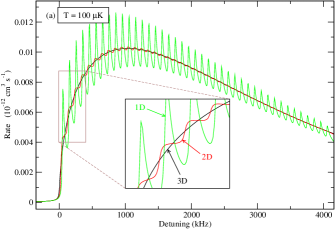
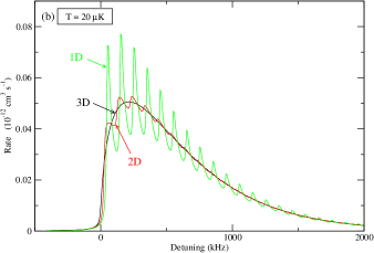
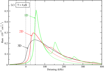
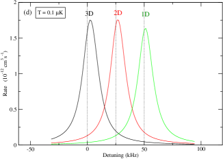
Figure 1: Photoassociation rate of Strontium 88 at low intensity ($l_{\textrm{opt}}=1$ Bohr $\approx$ 0.0529 nm) as a function of laser detuning, comparing free-space (3D), 1D-confinement (2D geometry) and 2D-confinement (1D geometry), with a trapping frequency $\Omega=2\pi\times 50$ kHz. Black curves are the free-space 3D prediction - Eq. (37). Red curves are the effective 3D rate in a 2D geometry - Eq. (31). Green curves are the effective 3D rate in a 1D geometry - Eq. (35). Panel (a) : $T=100\,\mu$K (free-space regime), Panel (b) : $T=20\,\mu$K; Panel (c) : $T=$ 4 $\mu$K (confinement-dominated regime), Panel (d) : $T=$ 0.1 $\mu$K (Quasi-2D or -1D regime). In the confinement-dominated regime, the approximate line shapes calculated from Eqs. (40-42) (considering only the trap ground-state contribution) are represented by dashed curves.

We illustrate the previous theory by considering alkaline-earth intercombination photoassociation in a tight optical lattice. An important feature of the intercombination line is the low spontaneous emission from the photoassociated state. While the natural width for allowed transitions is typically tens of MHz, the width of the intercombination lines is typically tens of kHz. This is on the same order of magnitude as the typical trapping frequency at the centre of each lattice cell. As a result, we expect a clear manifestation of the effects described in the previous section for alkaline-earth intercombination transitions. On the other hand, they should hardly be observable with allowed transitions, as they would be hidden by the large natural width.

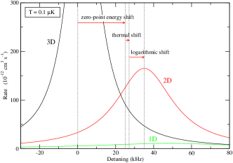
Figure 2: Same as Fig. 1d for higher intensity or stronger resonance ($l_{\textrm{opt}}=500$ Bohr $\approx$ 26.6 nm). The 2D and 1D lines are now saturated (especially the 1D line), in accordance with Eqs. (52) and (53), while the free-space line is not. The 2D line is also shifted according to Eq. (51). We indicated the three contributions to the shift by horizontal arrows.

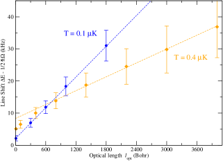
Figure 3: Shift $\Delta E$ of the photoassociation line in a 2D geometry with trap frequency $\Omega=2\pi\times 50$ kHz, as a function of optical length (proportional to photoassociation laser intensity). For convenience, we substracted the zero-point energy shift $\frac{1}{2}\hbar\Omega$ which is constant. The orange diamonds correspond to a temperature $T=0.4\,\mu$K, and the blue dots corresponds to a temperature $T=0.1\,\mu$K. These points are obtained by calculating the line shape using Eq. (46) and finding the shift numerically. For each point, we represented a vertical line whose length corresponds to one sixth of the photoassociation line width; this gives an indication of how accurately the shift can be determined experimentally. The dashed lines are obtained using the approximate formula Eq. (51).

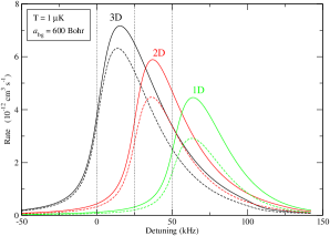
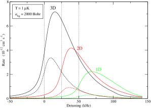
Figure 4: Photoassociation rates for Strontium 86 ($\Omega=2\pi\times 50$ kHz, $l_{\textrm{opt}}=10$ Bohr $\approx$ 0.0529 nm, $T=1\,\mu$K; conditions similar to the experiment of Ref. Zelevinsky et al. (2006)). Black curves are the free-space 3D rate prediction, red and green curves are the effective 3D rate from the 2D and 1D theories, using the effective scattering length (21); the dashed curves are obtained using the more usual expression (25) for the scattering length. Panel (a): assuming $a_{\textrm{bg}}=600$ Bohr $\approx$ 31.75 nm. Panel (b): assuming $a_{\textrm{bg}}=2000$ Bohr $\approx$ 105.8 nm. Note that the free-space rate does not depend on the background scattering length $a_{\textrm{bg}}$.

Figure 1 shows the effective photoassociation rate at different temperatures for a typical intercombination line of Strontium 88 in free space, 1D lattice, and 2D lattice. The scattering length of Strontium is taken to be 10 Bohr Mickelson et al. (2005) (1 Bohr $\approx$ 0.0529177 nm) and the spontaneous emission term $\gamma=15$ kHz Zelevinsky et al. (2006). The trapping frequency $\Omega$ is 2$\pi\times$50 kHz, and the optical length is set to 1 Bohr. The temperatures correspond to the three regimes discussed in Section II.6: free space ($T=100\,\mu$K and $T=20\,\mu$K), confinement-dominated ($T=4\,\mu$K ), and 2D regime ($T=0.1\,\mu$K ).

For $T=100\,\mu$K and $T=20\,\mu$K (Fig. 1a and 1b), one might expect the line shape to be very close to the free-space theory prediction. This is indeed the case in a 2D geometry. However, higher temperatures are needed to reach the free-space regime in a 1D geometry. For the temperatures considered here, we observe a lot of distinct spikes in the 1D photoassociation line. These spikes correspond to contributions from different trap states and are therefore separated by twice the frequency $\Omega$ of the trap - see Eq. (9) with $m=0$. There are similar contributions in the 2D case, but they tend to overlap, due to their width. In contrast, the spikes are very narrow in the 1D case, because the one-dimensional density of states scales like $1/\sqrt{E}$ (see, for instance, Eq.(44)), which enhances low-energy collisions. As a result each spike has a width close to the natural width of the resonance and is well separated from the others, even at relatively high temperatures (tens of $\mu$K) which are more than one order of magnitude larger than the natural width. This feature could be exploited to measure the position of the line at nearly the natural width precision, while operating at temperatures much larger than this width. Note that we have assumed ideal harmonic confinement, which is why the spikes are regularly spaced and well separated. Experimentally, only the first spikes should be visible, due to the anharmonicity of the lattice potential.

In the confinement-dominated regime (Fig. 1c), the line shape is dominated by the first spike (contribution from the trap ground state) and the line is clearly shifted due to the zero-point energy. In the 2D case, the density of states leads to a line which is more symmetric and narrower than in 3D, resulting in an increase of the photoassociation rate on resonance with respect to the free-space rate. This situation corresponds roughly to the experimental conditions of Ref. Zelevinsky et al. (2006). However, the experimental conditions were such that the 2D and 3D theory happened to predict very similar rates, and extra broadening mechanisms made it difficult to observe an unambiguous 2D line shape as in Fig. 1c. In the 1D case, the thermal distribution leads to an even narrower line and higher rate, as small collision energies are enhanced by the density of states.

In the quasi-2D or quasi-1D regime (Fig. 1d), the line is almost unbroadened by temperature and recovers its natural Lorentzian shape in all theories. The temperature is so low that there is almost one collision energy in the system: 0 in the 3D theory, $\frac{1}{2}\hbar\Omega$ in the 2D theory, and $\hbar\Omega$ in the 1D theory.

In Fig. 2, we consider a higher optical length ($l_{\textrm{opt}}=500$ Bohr), which can be reasonably attained using the intercombination lines close to thresold, or by increasing the photoassociation laser intensity. The line is now power-broadened, as predicted by Eqs. (52-53), while the free-space line is not. As explained before, the broadening is due to the zero-point momentum in the 2D case, and to fermionization in the 1D case. In the quasi-2D regime, the line is also shifted by the logarithmic term, according to Eq. (51). As suggested in Section II.7, this shift could be used as a way to measure the optical length. However, the line is progressively power-broadened as it is shifted. In Fig. 3, we plot the shift and width as a function of the optical length. Although the experiment may not be easy, this graph suggests that the shift should be observable.

We now illustrate the theory with the intercombination lines in Strontium 86. The background scattering length of this species has been found to be quite large, between 610 and 2300 Bohr Mickelson et al. (2005). As a result, the photoassociation line in the lattice is notably modified by the scattering length. In Fig. 4, we plotted the photoassociation rate for $a_{bg}=600$ Bohr and $a_{bg}=$ 2000 Bohr. The effect of the scattering length is clearly noticeable, as predicted qualitatively by Eqs. (54-55). As noted previousy, measurements of the rate for different lattice wave lengths might be able to give a better constraint on the scattering length.

We also plotted on Fig. 4 the effective rate obtained if one replaces the effective scattering length (21) by the more usual resonant scattering length (25). The latter appears to be insufficient to predict the correct rate for large scattering length, showing that in this particular case, one cannot simply extrapolate the original work of Refs. Petrov and Shlyapnikov (2001); Olshanii (1998) by replacing the scattering length by the resonant scattering length (25).

IV Conclusion

We investigated how photoassociation is affected by the confinement of a 1D or 2D optical lattice. We showed that effects are expected to be observable in the case of narrow resonances, like the intercombination lines found in alkaline-earth species. The main effects of confinement are: shift of the resonance (most importantly by the zero-point energy of the lattice), narrower lines, increase of power-broadening at low temperature, and direct sensitivity to a large value of the scattering length of the atoms. More specifically, a 2D confinement could significantly increase the spectroscopic resolution, making it possible to observe the natural line width at relatively high temperatures. At low temperature, a 1D confinement induces a shift of the line which is proportional to the intensity of the photoassociation laser. This shift could be used to determine the strength of a resonance, without having to measure the density of the system.