Phase transition and hysteresis in scale-free network traffic

Abstract

We model information traffic on scale-free networks by introducing the node queue length $L$ proportional to the node degree and its delivering ability $C$ proportional to $L$. The simulation gives the overall capacity of the traffic system which is quantified by a phase transition from free flow to congestion. It is found that the maximal capacity of the system results from the case of the local routing coefficient $\phi$ slightly larger than zero, and we provide an analysis for the optimal value of $\phi$. In addition, we report for the first time the fundamental diagram of flow against density, in which hysteresis is found, and thus we can classify the traffic flow with four states: free flow, saturated flow, bistable and jammed.

Complex networks can describe many natural and social systems in which lots of entities or people are connected by physical links or some abstract relations. Since the discovery of small-world phenomenon by Watts and Strogatz WS , appeared in Nature in 1998, and scale-free property by Barabási and Albert BA one year later in Science, complex networks have attracted growing interest among physics community BA2 ; BA3 ; Newman ; Newman2 ; Boccaletti . As pointed out by Newman, the ultimate goal of studying complex networks is to understand how the network effects influence many kinds of dynamical processes taking place upon networks Newman . One of the dynamical processes, traffic of information or data packets is of great importance to be studied for the modern society. Nowadays we rely greatly on networks such as communication, transportation, the Internet and power systems, and thus ensuring free traffic flow on these networks is of great significance and research interest. In the pass several decades, a great number of works on the traffic dynamics have been carried out for regular and random networks. Since the increasing importance of large communication networks with scale-free property such as the Internet PS , the traffic flow on scale-free networks has drawn more and more attention Sole ; Arenas ; Tadic ; Zhao ; Mukherjee ; Guimera ; Guimera2 ; Echen ; Wang ; Wang2 ; Yin ; YanGang ; deMenezes ; deMenezes2 ; Germano .

Researchers have proposed some models to mimic the traffic on complex networks by introducing the random generation and the routing of packets Sole ; Arenas ; Tadic ; Zhao ; Mukherjee ; Guimera ; Guimera2 . Arenas et al. suggest a theoretical measure to investigate the phase transition by defining a quantity Arenas , so that the state of traffic flow can be classified to the free flow state and the jammed state, where the free flow state corresponds to the number of created and delivered packet are balanced, and the jammed state corresponds to the packets accumulate on the network.

Many recent studies have focused on two aspects to control the congestion and improve the efficiency of transportation: modifying underlying network structures or developing better route searching strategies in a large network Kleinberg . Due to the high cost of changing the infrastructure, the latter is comparatively preferable. In this light, Echenique et al., Wang et al. and Yin et al. suggest traffic models based on the local information or the local integration of static and dynamic information Echen ; Wang ; Wang2 ; Yin . Yan et al. propose a efficient routing strategy based on the knowledge of the whole topology YanGang . They find that the efficient path results in the redistributing traffic loads from central nodes to other noncentral nodes, and the network capability in handling traffic flow is improved more than 10 times by optimizing the efficient path.

However, previous studies usually assumed that the capacity of each node, i.e., the maximum queue length of each node for holding packets, is unlimited and the node handling capability, that is the number of data packets a node can forward to other nodes each time step, is either a constant or proportional to the degree of each node. But, obviously, the capacity and delivering ability of a node are limited and variates from node to node in real systems, and in most cases, these restrictions could be very important in triggering congestion in the traffic system.

Since the analysis on the effects of the node capacity and delivering ability restrictions on traffic efficiency is still missing, we propose a new model for the traffic dynamics of such networks by taking into account the maximum queue length $L$ and handling capacity $C$ of each node. The phase transition from free flow to congestion is well captured and, for the first time, we introduce the fundamental diagram (flux against density) to characterize the overall capacity and efficiency of the networked system. Hysteresis in such network traffic is also produced.

To generate the traffic network, our simulation starts with the most general Barabási-Albert scale-free network model which is in good accordance with real observation of communication networks BA2 . In this model, starting from $m_{0}$ fully connected nodes, one node with $m$ links is added at each time step in such a way that the probability $\Pi_{i}$ of being connected to the existing node $i$ is proportional to the degree $k_{i}$ of the node, i.e. $\Pi_{i}={k_{i}\over\Sigma_{j}k_{j}}$, where $j$ runs over all existing nodes.

The capacity of each node is restricted by two parameters: (1) its maximum packet queue length $L$, which is proportional to its degree $k$ (a hub node ordinarily has more memory): $L=\alpha\times k$; (2) the maximum number of packets it can handle per time step: $C=\beta\times L$. Here $0<\beta\leq 1$ simply shows that the maximum number of handled packets is less than the maximum packet queue length $L$. Motivated by the previous models Sole ; Arenas ; Tadic ; Zhao ; Echen ; Wang ; Wang2 , the system evolves in parallel according to the following rules:

1. Add Packets - Packets are added with a given rate $R$ (packets per time step) at randomly selected nodes and each packet is given a random destination.

2. Navigate Packets - Each node performs a local search among its neighbors. If a packet’s destination is found in its nearest neighborhood, its direction will be directly set to the target. Otherwise, its direction will be set to a neighboring node $h$ with preferential probability: $P_{h}={k^{\phi}_{h}\over\Sigma_{i}k^{\phi}_{i}}$. Here the sum runs over the neighboring nodes, and $\phi$ is an adjustable routing parameter in that the packets are more likely to be forwarded to high degree nodes when $\phi>0$. It is assumed that the nodes are unaware of the entire network topology and only know the neighboring nodes’ degree $k_{i}$.

3. Deliver Packets – At each step, all nodes can deliver at most $C$ packets towards its destinations and FIFO (first-in-first-out) queuing discipline is applied at each node. When the queue at a selected node is full, the node won’t accept any more packets and the packet will stay at the site and wait for the next opportunity to be forwarded. Once a packet arrives at its destination, it will be removed from the system. As in other models, we treat all nodes as both hosts and routers for generating and delivering packets.

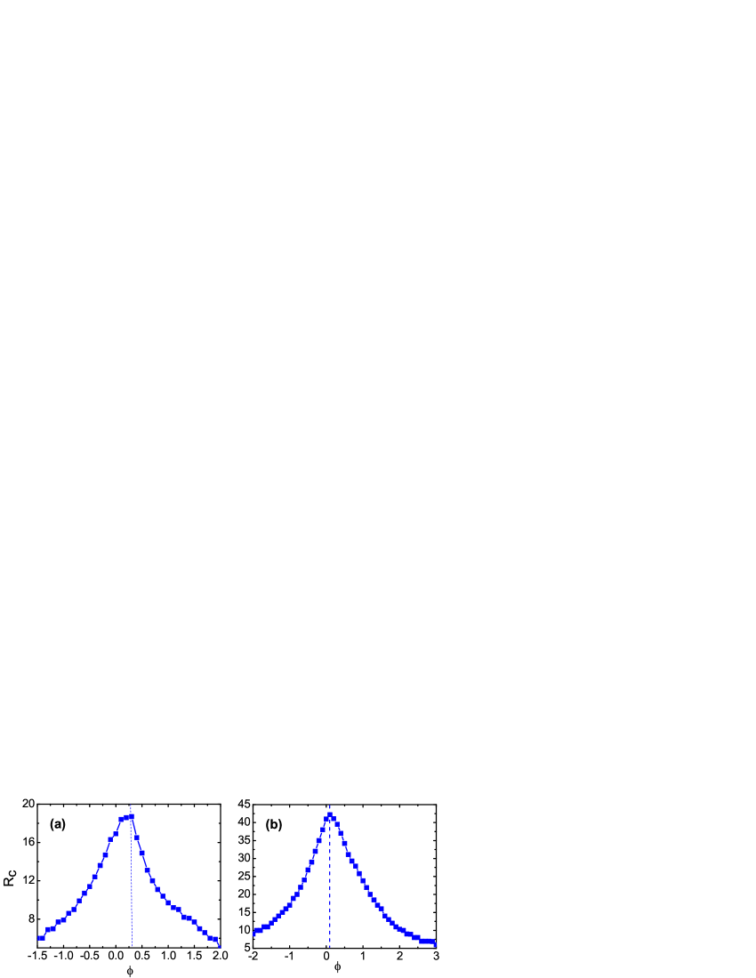
Figure 1: (color online). The overall capacity of a network with $N=1000$, $m0=m=5$, $\alpha=1$(a), $\alpha=2$(b) and $\beta=0.2$. The capacity is characterized by the critical value of $R_{c}$ for different $\phi$. In (a), $\alpha=1$, $\phi_{optimal}=0.3$ and $R_{c}^{max}=18.7$. In (b), $\alpha=2$, $\phi_{optimal}=0.1$ and $R_{c}^{max}=42.2$. In both cases, the maximum of $R_{c}$ corresponds to a $\phi$ slightly greater than zero marked by a dash line. The data are obtained by averaging $R_{c}$ over 10 network realizations.

We first simulate the traffic on a network of $N=1000$ nodes with $m0=m=5$. To characterize the system’s overall capacity, we first investigate the increment rate $\eta$ of the number of packets in the system: $\eta(R)=\lim_{t\rightarrow\infty}{\langle\Delta N_{p}\rangle\over\Delta t}$. Here $\Delta N_{p}=N_{p}(t+\Delta t)-N_{p}(t)$ with $\langle...\rangle$ takes average over time windows of width $\Delta t$. Obviously, $\eta(R)=0$ corresponds to the cases of free flow state, which is attributed to the balance between the number of added and removed packets at the same time. As $R$ increases, there is a critical $R_{c}$ at which $N_{p}$ runs quickly towards the system’s maximum packet number and $\eta(R)$ increases suddenly from zero, which indicates that packets accumulate in the system and congestion emerges and diffuses to everywhere.

Hence, the system’s overall capacity can be measured by the critical value of $R_{c}$ below which the system can maintain its efficient functioning. Fig.1 depicts the variation of $R_{c}$ versus $\phi$. The maximum overall capacity occurs at $\phi$ slightly greater than $0.0$ with $R_{c}^{max}=18.7$ at $\phi=0.3$ for $\alpha=1$ (a) and $R_{c}^{max}=42.2$ at $\phi=0.1$ for $\alpha=2$ (b). The results are averaged from 10 simulations.

The analytical estimation of $R_{c}$ is too complicated for our routing model. In a recent paper Germano , Germano and de Moura present analytical work on the rather simple traffic of particle hopping in complex networks. In the following, we provide an analysis for the optimal value of $\phi$ corresponding to the peak value of $R_{c}$. In the case of $\phi=0$, packets perform random-like walks if the maximum queue length restriction of each node is neglected. The random walk process in graph theory has been extensively studied. A well-known result valid for our analysis is that the time the particle spends at a given node is proportional to the degree of such node in the limit of long times Bollob . Similarly, in the process of packet delivery, the number of received packets (load) of a given node averaging over a period of time is proportional to the degree of that node. Note that the packets delivering ability $C$ of each node assumed to be proportional to its degree, so that the load and delivering ability of each node are balanced, which leads to a fact that no congestion occurs earlier on some nodes with particular degree than on others. Since in our traffic model, an occurrence of congestion at any node will diffuse to the entire network ultimately, no more easily congested nodes brings the maximum network capacity. However, taking the maximum queue length restriction into account, short queue length of small degree nodes make them more easily jammed, so that routing packets preferentially towards large degree nodes slightly, i.e., $\phi$ slightly larger than zero, can induce the maximum capacity of the system.

This also explain the difference in the position of $R_{c}^{max}$ of Fig.1(a) and Fig.1(b). Comparing with the case of $\alpha=2$, the small degree nodes are more easy to jam when $\alpha=1$, so a greater $\phi$ is needed to achieve a more efficient functioning of the system. One can also conclude that the optimal $\phi$ will be zero if $\alpha$ is large enough.

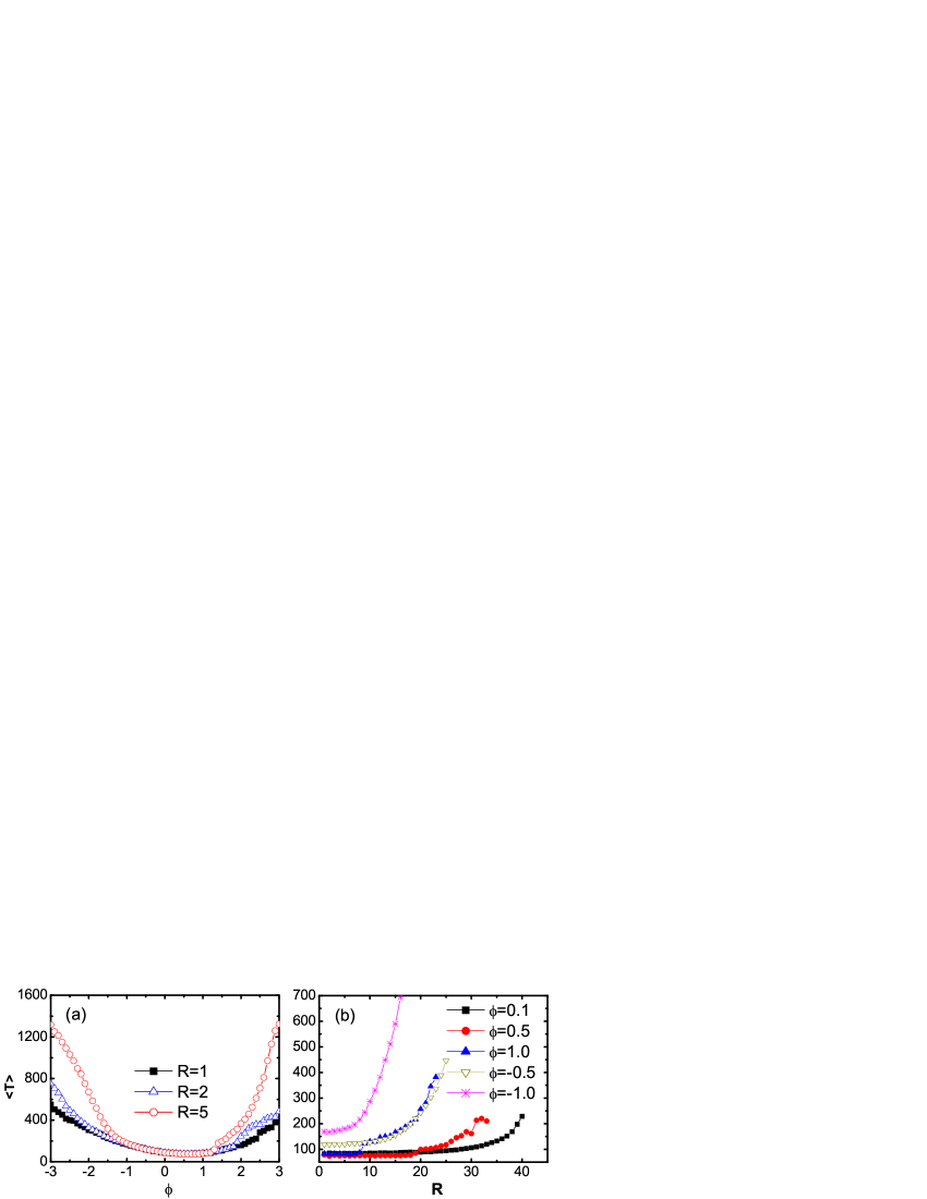
Figure 2: (color online). Average travel time for a network with $N=1000$, $m_{0}=m=5$, $\alpha=2$ and $\beta=0.2$. (a) Average travel time $\langle T\rangle$ versus $\phi$ for $R=1$, $2$ and $5$. The data are truncated because the system jams when $\phi$ is either too large or too small. (b) The variation of $\langle T\rangle$ versus $R$ when $\phi$ is fixed. The data are also truncated when the system jams.

Then we simulate the packets’ travel time which is also important for measuring the system’s efficiency. In Fig.2(a), we show the average travel time $\langle T\rangle$ versus $\phi$ under the conditions of $R=1$, $2$ and $5$. In the free-flow state, almost no congestion on nodes occurs and the time for packets waiting in the queue is negligible, therefore, the packets’ travel time is approximately equal to their actual path length in map. But when the system approaches a jammed state, the travel time will increase rapidly. One can see that when $\phi$ is slightly greater than zero, the minimum travel time is obtained. In Fig.2(b), the average travel time is much longer when $\phi$ is negative than it is positive. These results are consistent with the above analysis that a maximum $R_{c}$ occurs when $\phi$ is slightly greater than zero. Or, in other words, this can also be explained as: when $\phi>0$, packets are more likely to move to the nodes with greater degree (hub nodes), which enables the hub nodes to be efficiently used and enhance the system’s overall capability; but when $\phi$ is too large, the hub nodes will more probably get jammed, and the efficiency of the system will decrease.

Finally, we study the fundamental diagram of network traffic with our model. Fundamental diagram (flux-density relation) is one of the most important criteria that evaluates the transit capacity for a traffic system. Obviously, if the nodes are not controlled with the queue length $L$, the network system will not have a maximum number of packets it can hold and the packet density can not be calculated, so that the fundamental diagram can not be reproduced.

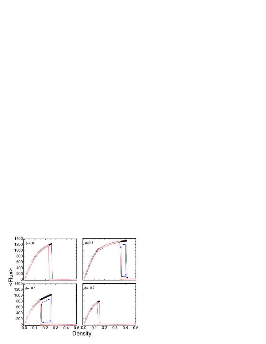
Figure 3: (color online). Fundamental diagram for a $N=1000$ network with $m0=m=5$, $\alpha=1$, $\beta=0.2$, and different $\phi$. The data are averaged over 10 typical simulations on one realization of network. In each chart, the solid square line shows the flux variation when adding packets to the system (increase density), while the empty circle line shows the flux variation when drawing out packet from the system (decrease density). The sudden transition density values are: 0.26 and 0.23 ($\phi=0.0$), 0.40 and 0.34($\phi=0.3$), 0.26 and 0.15($\phi=-0.5$), 0.15 and 0.13($\phi=-0.7$). For different realizations of network, the fundamental charts are similar, but with small difference in the transition values. The arrows in charts of $\phi=0.3$ and $-0.5$ are showing the hysteresis for guide of eyes.

To simulate a conservative system, we count the number of removed packets at each time step and add the same number of packets to the system at the next step. The flux is calculated as the number of successfully delivered packets from node to node through links per step. In Fig.3, the fundamental diagrams for $\phi=0.0,0.3,-0.5$ and $-0.7$ are shown.

The curves of each diagram show four flow states: free flow, saturate flow, bistable and jammed. For simplicity, we focus on the $\phi=0.3$ chart with the maximum $\langle Flux\rangle=1319$ in the following description. As we can see, when the density is low (less than $\approx 0.10$), all packets move freely and the flux increases linearly with packet density, which is attributed to a fact that in the free flow state, all nodes are operated below its maximum delivering ability $C$. Then the flux’s increment slows down and the flux gradually comes to saturation ($0.10\sim 0.34$), where the flux is restricted mainly by the delivering ability $C$ of nodes.

At the region of medium density, the model reproduces an important character of traffic flow - “hysteresis”, which can be seen that two branches of the fundamental diagram coexist between $0.34$ and $0.40$. The upper branch is calculated by adding packets to the system, while the lower branch is calculated by removing packets from a jammed state and allowing the system to relax after the intervention. In this way a hysteresis loop can be traced (arrows in Fig.3), indicating that the system is bistable in a certain range of packet density. As we know so far, it is the first time that the hysteresis phenomenon is reported in the scale-free traffic system.

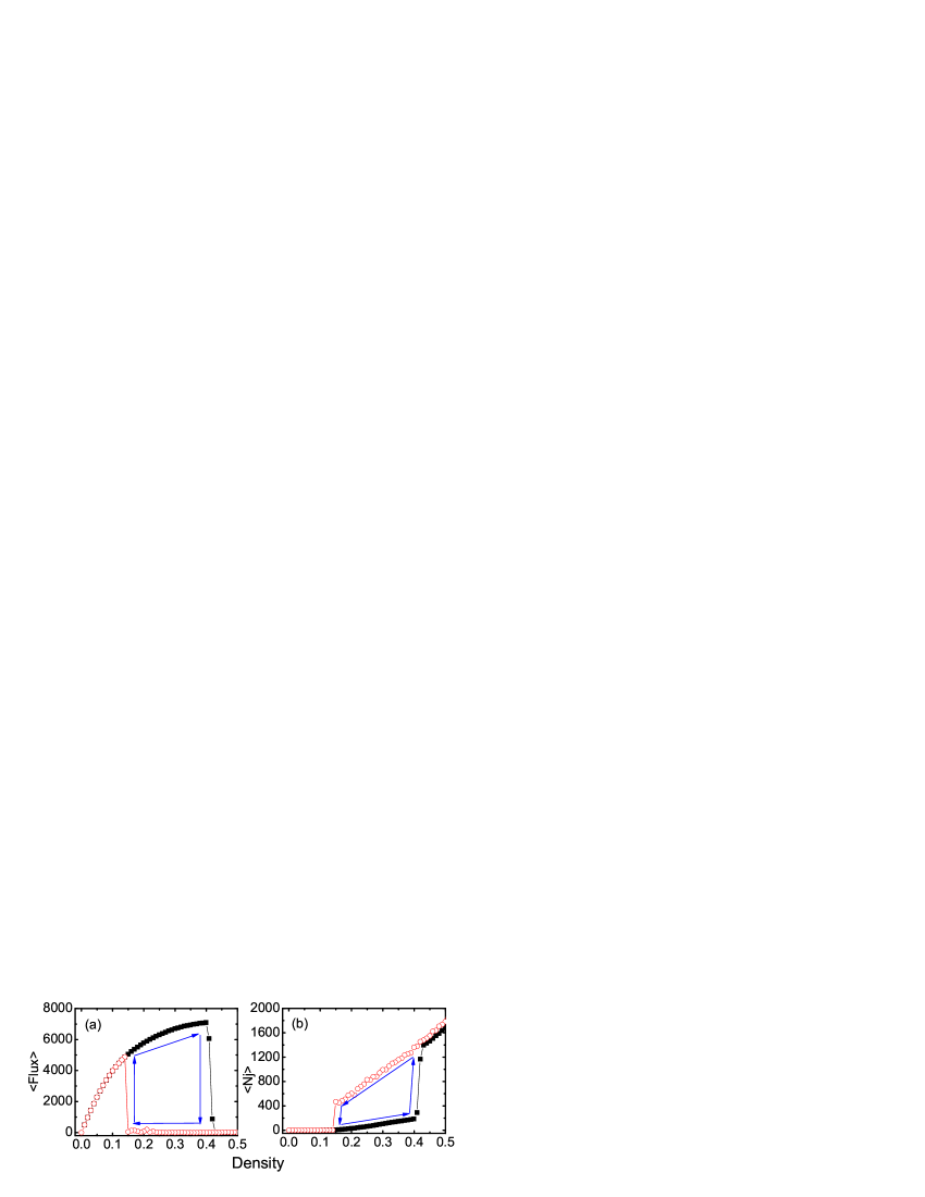
Figure 4: (color online). (a) Fundamental diagram for a $N=5000$ network with $m0=m=5$, $\alpha=1$, $\beta=0.2$ and $\phi=0.1$. (b) The averaged number of jammed nodes $\langle N_{jv}\rangle$. The symbols for increasing/decreasing density are the same as in Fig.3. One can see that the two sudden change points $0.40$ and $0.14$ in both charts are equal. The arrows are showing the hysteresis for guide of eyes.

One can also notice that when $\phi=0.3$, the maximum saturated $\langle Flux\rangle$ is higher than others, and the saturated flow region is much boarder than the cases of $\phi=0.0,-0.5$ and $-0.7$. All these results show that the system can operate better when $\phi$ is slightly greater than zero, which is also in agreement with the simulation result of $R_{c}$ in Fig.1.

In order to test the finite-size effect of our model, we simulate some systems with bigger size. The simulation shows similar phase transition and hysteresis in fundamental diagram as shown in Fig.4(a).

The flux’s sudden drop to a jammed state from a saturated flow indicates a first order phase transition, which can be explained by the sudden increment of full (jammed) nodes in the system (See Fig.4(b)). According to the evolutionary rules, when a given node is full, packets in neighboring nodes can not get in the node. Thus, the packets may also accumulate on the neighboring nodes and get jammed. This mechanism can trigger an avalanche across the system when the packet density is high. As shown in Fig.4(b), the number of full nodes increase suddenly at the same density where the flux drop to zero and almost no packet can reach its destination. As for the lower branch in the bistable state, starting from an initial jammed configuration, the system will have some jammed nodes that are difficult to dissipate. Clearly, these nodes will decrease the system efficiency by affecting the surrounding nodes until all nodes are not jammed, thus we get the lower branch of the loop.

In conclusion, a new model for scale-free network traffic is proposed to consider the nodes’ capacity and delivering ability. In a systemic view of overall efficiency, the model reproduces several significant characteristics of network traffic, such as phase transition, and for the first time, the fundamental diagram for networked traffic system. Influenced by two factors of each node’s capability and navigation efficiency of packets, the optimal routing parameter $\phi$ is found to be slightly greater than zero to maximize the whole system’s capacity. A special phenomenon - the “hysteresis” - is also reproduced in the typical fundamental diagram, indicating that the system is bistable in a certain range of packet density. It is the first time that the phenomenon is reported in networked traffic system. For different packet density, the system can self-organize to four different phases: free-flow, saturated, bistable and jammed.

Our study may be useful for evaluating the overall efficiency of networked traffic systems, and the results may also shed some light on alleviating the congestion of modern technological networks.

This work is funded by National Basic Research Program of China (No.2006CB705500), the NNSFC under Key Project No.10532060, 10635040, Project Nos.70601026, 10672160, 10404025, the CAS President Foundation, and by the Chinese Postdoctoral Research Foundation (No.20060390179). Y.-H. Wu acknowledges the support of the Australian Research Council through a Discovery Project Grant.

References

- (1) D.J. Watts and S.H. Strogatz, Nature(London) 393,440 (1998).
- (2) A.-L. Barabási, R. Albert, Science 286, 509 (1999).
- (3) R. Albert, H. Jeong, and A.-L. Barabási, Nature (London) 401, 103(1999).
- (4) R. Albert, A.-L. Barabási, Rev. Mod. Phys. 74, 47(2002).
- (5) M.E.J. Newman, Phys. Rev. E 64, 016132 (2001).
- (6) M.E.J. Newman, SIAM Review 45, 167(2003).
- (7) S. Boccaletti, V. Latora, Y. Moreno, M. Chavez, D.-U. Hwang, Physics Reports 424, 175(2006).
- (8) R. Pastor-Satorras and A. Vespignani, Evolution and Structure of the Internet: A Statistical Physics Approach (Cambridge University Press, Cambridge, 2004).
- (9) R.V. Sole, S. Valverde, Physica A 289, 595 (2001).
- (10) A. Arenas, A. Díaz-Guilera, and R. Guimerá, Phys. Rev. Lett. 86, 3196 (2001).
- (11) B. Tadić, S. Thurner, G.J. Rodgers, Phys. Rev. E 69, 036102 (2004).
- (12) L. Zhao, Y.C. Lai, K. Park, N. Ye, Phys. Rev. E 71, 026125 (2005).
- (13) G. Mukherjee, S.S. Manna, Phys. Rev. E 71, 066108 (2005).
- (14) R. Guimerà, A. Díaz-Guilera, F. Vega-Redondo, A. Cabrales, and A. Arenas, Phys. Rev. Lett. 89, 248701 (2002).
- (15) R. Guimerà, A. Arenas, A. Díaz-Guilera, F. Giralt, Phys. Rev. E 66, 026704 (2002).
- (16) P. Echenique, J. Gómez-Gardeñes, Y. Moreno, Phys. Rev. E 70, 056105 (2004); P. Echenique, J. Gómez-Gardeñes, Y. Moreno, Europhys. Lett. 71(2), 325(2005).
- (17) W.X. Wang, B.H. Wang, C.Y. Yin, Y.B. Xie, T. Zhou, Phys. Rev. E. 73, 026111 (2006).
- (18) W.X. Wang, C.Y. Yin, G. Yan, B.H. Wang, Phys. Rev. E 74, 016101 (2006).
- (19) C.Y. Yin, B.H. Wang, W.X. Wang, G. Yan, H.J. Yang, Eur. Phys. J. B 49, 205 C211 (2006).
- (20) G. Yan, T. Zhou, B. Hu, Z.Q. Fu, B.H. Wang, Phys. Rev. E 73, 046108 (2006).
- (21) M.A. deMenezes, A.-L. Barabási, Phys. Rev. Lett. 92, 028701(2004).
- (22) M.A. deMenezes, A.-L. Barabási, Phys. Rev. Lett. 93, 068701(2004).
- (23) R. Germano, A.P.S. de Moura, Phys. Rev. E 74, 036117 (2006).
- (24) J.M. Kleinberg, Nature(London) 406, 845(2000).
- (25) B. Bollobás, Modern Graph Theory (Springer-Verlag, New York, 1998).