Numerical calculation of classical and non-classical electrostatic potentials

Abstract

We present a numerical exercise in which classical and non-classical electrostatic potentials were calculated. The non-classical fields take into account effects due to a possible non-zero photon rest mass. We show that in the limit of small photon rest mass, both the classical and non-classical potential can be found by solving Poisson’s equation twice, using the first calculation as a source term in the second calculation. Our results support the assumptions in a recent proposal to use ion interferometry to search for a non-zero photon rest mass.

I Introduction

Although classical electromagnetism forbids electrostatic fields inside empty conducting shells, quantum mechanics suggests that small fields might exist. In the spirit of Yukawa’s particle-exchange theory of forces Yukawa (1964), a modified version of Maxwell’s equations was derived to account for a possible non-zero rest mass of the photon, the exchange particle of the Coulomb force Jackson (1975). Because a finite photon mass would limit the range of the Coulomb force, these equations violate Gauss’s law and make these fields possible.

The experimental search for deviations from Coulomb’s inverse-square law goes back as early as 1769 Cavendish (1879); Jackson (1975); Elliott (1966). Although no field has been found at the sensitivity level of these experiments, based on the predicted sensitivity of the experiments an upper limit on the photon rest mass has been determined. The most recent tests of Coulomb’s law were limited by the sensitivity of the voltage-measurement electronics and possible back-action of the measurement process on the potentials being measured Crandall (1983); Williams et al. (1971).

Progress on these experiments has been slow — the limit on the rest mass of a photon from these types of experiments has decreased by only a factor of 2.5 in the last 35 years. We recently proposed to use ion interferometry to improve this measurement by several orders of magnitude Neyenhuis et al. (2006). In this experiment, a voltage would be applied across a concentric pair of conducting cylindrical shells. A beam of ions traveling through the inner shell would be split and recombined using either physical gratings or laser beams. A non-zero electric field in the shell would induce a phase shift between the arms of the interferometer, resulting in a shift in the interference pattern.

While investigating the feasibility of the experiment, we performed several numerical calculations of classical and non-classical electrostatic potentials in the proposed apparatus. In this paper we discuss the methods and results of these calculations.

II Definition of the Problem

In the proposed experiment, a non-zero electric field will be searched for inside the inner of two concentric cylindrical conductors held at different voltages. The inner conductor’s end caps would have several small holes to allow passage of the ions and to allow laser beams and/or wires to enter. For the experiment to work, the fringing fields "leaking" through these holes must be small compared to the non-classical field under study. In addition, the calculations in Neyenhuis et al. (2006) assume that the non-classical part of the potential between the interferometer gratings is approximately that of an infinite cylinder. To verify that these conditions are met, we performed several numerical calculations.

The setup assumed for these calculations is illustrated in Fig. 1. The inner conducting shell was assumed to be a thin-walled 2.6 m long cylinder, 27 cm in radius. It is capped on either end with conducting disks, also 27 cm in radius. These disks are 20 cm long to reduce fringing fields through the holes. This inner shell is surrounded by a second conducting tube with end caps. The outer tube is 3.06 m long with an inner radius of 30 cm, giving a 3 cm clearance between the inner and outer shells on all sides. The inner shell was assumed to be at a voltage $V$ relative to the outer shell, which was assumed to be grounded. In an actual experiment, $V$ will likely be hundreds of kV. But because all of the potentials we calculated scale linearly with $V$, we set $V=1\textrm{ V}$ for our calculations, and then scaled the results.

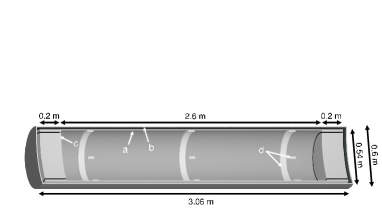
Figure 1: Layout of conductors. This scale figure gives a cut-away perspective view of the conductors which enforce the boundary conditions assumed in our calculations. Arrows point out (a) the inner conducting cylinder, (b) the outer conducting cylinder, (c) the disk which caps one end of the inner conductor, and (d) one of the three sets of additional conductors inserted into our calculation to explore the effect of mounting objects inside the inner conductor.

For simplicity we performed our calculations for a cylindrically-symmetric geometry, replacing the holes in the inner conductor’s end caps with radial slices generated by rotating a 1 cm hole about the axis at a radius of 25 cm. As such, the fringing fields that we calculate will be significantly larger than the actual fields in the real apparatus, and the calculation should be considered a “worst case” estimate.

III Equations for Classical and Non-classical Potentials

To find the classical fringing-field potential $\phi_{c}$ from a given set of static boundary conditions we use Laplace’s equation. For the non-classical field, we use the counterpart to Laplace’s equation for massive photons:

$$\nabla^{2}\phi-\mu^{2}\phi=0.$$ (1)

The constant $\mu$ in this equation is related to the photon rest mass $m_{\gamma}$ by the relation $\mu=m_{\gamma}c/\hbar$.

For the non-classical calculation, instead of solving for $\phi$, we solved for the deviation from the classical potential $\phi_{p}=\phi-\phi_{c}$. With this definition, Eq. 1 becomes

$$\nabla^{2}\phi_{c}+\nabla^{2}\phi_{p}-\mu^{2}\phi_{c}-\mu^{2}\phi_{p}=0.$$ (2)

Laplace’s equation states that $\nabla^{2}\phi_{c}=0$, so the first term in the above equation is zero. Also, since $\mu$ is known to be very small, we expect $\phi$ to be approximately equal to $\phi_{c}$. This implies that $\phi_{p}$ will be very small compared to $\phi_{c}$. As such, we can drop the last term. And since we don’t know a-priori what $\mu$ is equal to, we will normalize our equation by defining a new parameter $\phi_{s}=\phi_{p}/\mu^{2}$. Making this substitution and cancelling out the $\mu^{2}$ in both terms we get

$$\nabla^{2}\phi_{s}=\phi_{c}$$ (3)

Equation 3 is simply Poisson’s equation with $\phi_{c}$ playing the part of the charge distribution. As such, our simulation need only to be able to solve one equation,

$$\nabla^{2}\phi_{x}=y.$$ (4)

To calculate the classical potential $\phi_{c}$, we simply replace $\phi_{x}$ with $\phi_{c}$ and insert $y=0$ into this equation. To calculate the non-classical part of the potential, we first calculate $\phi_{c}$. Then we then replace $\phi_{x}$ with $\phi_{s}$, and insert our previously calculated values for $\phi_{c}$ as the source term $y$. For an axially-symmetric system, Eq. 4 can be written as a two-dimensional equation in cylindrical coordinates:

$$\frac{1}{r}\frac{\partial\phi_{x}}{\partial r}+\frac{\partial^{2}\phi_{x}}{\partial r^{2}}+\frac{\partial^{2}\phi_{x}}{\partial z^{2}}=y,$$ (5)

where $r$ and $z$ are the radial and axial coordinates.

Note that if $\mu\neq 0$, a constant potential is not a solution to Eq. 1, and we are not free to arbitrarily define the outer conductor to be at $V_{g}=0$. But if this conductor is Earth grounded, due to the huge capacitance of the Earth it is reasonable to assume that $V_{g}$ will remain fairly constant as the voltage on the inner conductor is changed. In the proposed experiment the inner conductor’s voltage relative to the outer conductor would be periodically reversed. Rather than measuring the field inside the conductor, the difference between the field before and after the reversal would be measured. In this measurement the the unknown voltage offset $V_{g}$ will cancel. As such, setting $V_{g}=0$ in our calculations still gives us meaningful results.

IV Methodology

We did our calculations using a finite difference method, in which the potential is calculated at points on a grid. Derivatives are approximated to second order from adjacent points on the grid. Our grid was evenly spaced in both dimensions, with points separated by a distance $a$. The potential $\phi_{x}$ at each point on the grid will be written as $\phi_{i,j}$ and the source term $y$ at each point as $y_{i,j}$, where $i$ and $j$ are integers labeling the point. We will define $i=j=0$ at the center of the conducting shells, such that the actual coordinates of each grid point are equal to $r_{i}=ai$ and $z_{j}=aj$. Using these definitions, Eq. 5 can be approximated by the equation

$$\frac{\phi_{i+1,j}-\phi_{i-1,j}}{2ar_{i}}+\frac{\phi_{i+1,j}-2\phi_{i,j}+\phi_{i-1,j}}{a^{2}}$$

$$+\frac{\phi_{i,j+1}-2\phi_{i,j}+\phi_{i,j-1}}{a^{2}} = y_{i,j}.$$ (6)

This can be solved for $\phi_{i,j}$ in terms of the known quantity $y_{i,j}$ and the value of $\phi_{x}$ at adjacent grid points:

$$\phi_{i,j} = \frac{1}{4}\bigg{[}\left(1+\frac{a}{2r_{i}}\right)\phi_{i+1,j}+\left(1-\frac{a}{2r_{i}}\right)\phi_{i-1,j}$$ (7)

$$\,\,\,\,\,\,\phi_{i,j+1}+\phi_{i,j-1}-a^{2}y_{i,j}\bigg{]}.$$

We began our simulation with an arbitrary value of $\phi_{i,j}$ at each grid point. Then using Gauss-Seidel iteration Press et al. (1992), this equation was evaluated at each point to produce an updated value of $\phi_{i,j}$. After many iterations, $\phi_{i,j}$ eventually converged to the correct values to solve Eq. 6. To accelerate convergence, we used the successive over-relaxation method Press et al. (1992).

One group of points which requires attention are the points for which $i=0$. Because $r$ is always positive in cylindrical coordinates, $\phi_{i,j}$ is not defined for negative values of $i$. But there is effectively no difference between cylindrical and Cartesian coordinates for the row of points along the axis. So for these points we calculated derivatives using Cartesian coordinates knowing that the points directly below the axis and just into or out of the two-dimensional grid should have the same value as the point directly above each point on the axis. This gives the equation

$$\phi_{0,j}=\frac{1}{6}\left(4\phi_{1,j}+\phi_{0,j+1}+\phi_{0,j-1}\right).$$ (8)

In addition to axial symmetry, the conductors have mirrored symmetry about their center. This allows us to throw away all of the grid points with $j<0$, cutting the number of grid points in half. Doing this requires us to treat the $j=0$ points differently, because our grid no longer contain values for $\phi_{i,-1}$. By symmetry we know that $\phi_{i,j}=\phi_{i,-j}$. This allows us to replace $\phi_{i,-1}$ with $\phi_{i,1}$ in Eq. 7. The point $\phi_{0,0}$ is a special point, being both a member of the $r=0$ and $z=0$ groups of points. For this point we use Eq. 8, but substitute $\phi_{0,1}$ for $\phi_{0,-1}$.

After every 100 iterations, the program calculated an estimated error at each point by evaluating Eq. 7 at each point without changing any values on the grid. We defined the estimated fractional error to be

$$\left|\frac{\phi_{i,j}-\Phi_{i,j}}{\phi_{i,j}}\right|,$$

where $\phi_{i,j}$ is the actual value at grid point ($i$,$j$) and $\Phi_{i,j}$ is the value calculated from Eq. 7. If there were no points on the grid with a fractional error larger than $10^{-8}$, the simulation terminated.

While experimenting with different conductor geometries, we significantly decreased the required computation time by successively reducing the size of the grid in the axial direction. This was done by finding columns which had already converged near their final value and then using these values as the new boundary conditions for a problem involving a smaller grid. To do this the program used a variable $jmax$, initialized to the largest $j$ index on the grid, and only updated points with $j\leq jmax$. After each set of 100 iterations the program stopped and calculated the fractional error for each of the points with $j=jmax$. If the fractional error at every point in this column was smaller than $10^{-8}$, the program would reduce $jmax$ by one, thereby reducing the effective size of the grid. The program then repeated this process until it found a column which contained at least one point who’s fractional error was larger than the specified value. Then the over-relaxation parameter was re-calculated and the next set of 100 iterations was performed. This process is illustrated in Fig. 2.

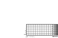
Figure 2: Reducing the grid size. In this process the fractional error of the outermost column of points (the dark grey column) is evaluated. If the fractional error for each of these points is less than a set value, the grid size is reduced and the next column of points (the medium grey column) is evaluated. If the error for each point in this column is smaller than the set value, the grid is reduced again and the next column (the light grey column) is evaluated. This process continues until a column is found which has at least one point with a fractional error larger than the specified limit. In this example, the right-most white column was the first column found to have a point with a fractional error above the set limit, and the grid was reduced in the direction of the arrow to the dashed line.

The error introduced by stepping in should be negligible; if a column has converged to within a factor $f$ of its final value, the error introduced onto other points by “freezing” this column should be of order $f$. Therefore, for a grid with $N_{z}$ columns, the largest fractional error introduced anywhere on the grid by this method should be on the order of $f\sqrt{N_{z}}$ if the errors are assumed to be random, and on the order of $fN_{z}$ or smaller otherwise.

Because we have not done a rigorous theoretical study of this method, once we had decided on the final geometry for our conductors we verified our calculations by performing additional computations which did not use this “stepping in” method. The result of these calculations were identical to those done with the stepping-in technique to the seven digits of precision saved at the end of the calculations.

V Classical Fringing-Field Potential

For the classical fringing-field calculation we are mainly interested in how the potential inside the inner conductor varies from $V$, the voltage of the inner conductor. To keep round-off error from completely masking these variations, we made use of the fact that classical electromagnetism allows us to arbitrarily add a constant potential. So rather than solving Laplace’s equation for $\phi_{c}$, we instead solved for $\Delta\phi_{c}=\phi_{c}-V$ using the same equation but different boundary conditions — $-V$ on the outer conductor and $0$ on the inner conductor. This way we found small deviations from zero rather than a finite potential.

The results of this calculation are shown in Fig. 3(a). We have verified that the errors due to a finite grid are negligible by performing this calculation with other grid spacings. If the grid spacing $a$ is increased by a factor of 3, $\Delta\phi_{c}$ at the center of the conductors changes by 9%. If $a$ is increased by a factor of 1.5, it changes by only 1.3%. We fit these three results to a power law, and found that the fit is in good agreement with a fourth data set data in which $a$ is increased by a factor of 6. From this fit we estimate an error on the order of 0.3%.

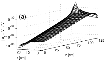
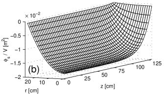
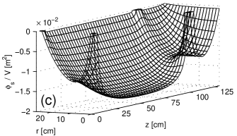
Figure 3: The results of the numerical calculations. All calculations were done with a grid spacing of $a=1.67\times 10^{-2}$ cm. Only the region inside the inner conductor is shown. In (a) a semi-log plot of the classical fringing-field potential is shown. The peak in the upper right-hand corner is at the location of the radial slice in the end cap. In (b) the non-classical potential $\phi_{s}$ is plotted. Frame (c) shows the effect of additional conducting objects inside the inner shell.

To verify the validity of our results we used a series solution to calculate the field inside of the inner conductor assuming that the inner conductor was grounded, and that the potential inside of the radial slices in the end caps was a fixed constant. This calculation showed that the potential at the center of the tube would be $4.5\times 10^{-7}$ times the potential inside the radial slices, in good agreement with our numerical calculation. We also found a series solution for the field between two grounded cylinders with a fixed potential applied to the gap at the ends. The length of the cylinders was assumed to be equal to the sum of the lengths of the two end caps, with a gap between them equal in size to the radial slice in the end caps. The field in the center of the gap turned out to be $2\times 10^{27}$ times smaller than the potential at the end, also in agreement with our numerical calculation.

VI Non-Classical Potential

To calculate $\phi_{s}$, we set $y=\phi_{c}$ in Eq. 3 and used the same methods discussed above. Since the potential on the conducting surfaces is given, the deviation from the classical potential should be zero on these surfaces. So the boundary conditions for the $\phi_{s}$ calculation were that $\phi_{s}=0$ on both of the conductors.

The source term $y$ in this calculation is equal to $\phi_{c}$. We can obtain this by adding $V$ to our already completed calculation of $\Delta\phi_{c}$. Inside the inner conductor, where $\Delta\phi_{c}$ is very small, this results in values accurate to the total precision allowed by the double-precision floating-point format. But between the two conductors, adding $V$ to $\Delta\phi_{c}$ results in lost precision. We are only interested in the fields inside the inner conductor, which should not be affected by this lost precision — the non-classical potential is predominantly generated by the local source term $y$ rather than from fringing fields generated outside the inner conductor. But to be extra careful we also calculated $\phi_{c}$ directly using the correct boundary conditions (the inner conductor at $V$ and the outer one at $0$), and used these values wherever $\phi_{c}$ was less than $V/2$.

The results of this calculation are shown in Fig. 3(b). Figure 3(c) shows the results of a similar calculation in which additional conductors were added to simulate optics and other objects inside the inner shell. These conductors consisted of a ring and a cylinder at the three locations where gratings would be positioned in the interferometer. The rings were assumed to be 6 cm wide and 1.5 cm thick, just touching the inner shell, and the cylinders to be 6 cm long and 1.5 cm in radius, centered on the axis of the inner shell, as shown in Fig. 1. These conductors were assumed to be at the same potential as the inner shell.

We estimate the error in these calculation to be very small — to the seven digits output by our program there was no change in $\phi_{s}$ when we increased the grid spacing by a factor of 3.

VII Implications

The fields are compared in Fig. 4. While this figure shows the potential at each point moving radially from the axis, for the proposed ion interferometer experiment, all that is important is the field at the location of the ion beam. As such, the most important information in this figure is the radial slope of the potential at $r=25\textrm{ cm}$.

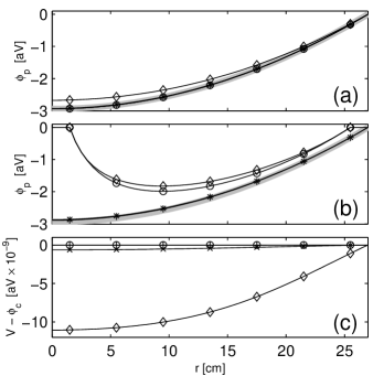
Figure 4: Comparing the different potentials. The potential is plotted as a function of radius at four different points along the axis. In (a) the non-classical field is shown. In (b) the non-classical field is shown for the case in which additional conductors have been placed inside the inner shell. In (c) the classical field is shown. The lines marked with circles and diamonds are at axial distances of 0 and 100 cm from the center of the conductors — the locations of the gratings. The lines marked with $+$ and $\times$ are at axial distances of 33 and 67 cm, respectively. All potentials were plotted assuming that $V=200\,\textrm{kV}$ and $\mu=2.8\times 10^{-11}\textrm{ m}^{-1}$. The thick grey lines in (a) and (b) represent the analytical solution for the non-classical field inside of an infinite cylinder.

In Fig. 4(a) we see that the non-classical field is approximated very well by the field of an infinite cylinder. In Fig. 4(b) we see that although the effect of small objects inside the shell on the non-classical potential is not negligible, it should not greatly change the sensitivity of the experiment as long as care is taken. Because axial symmetry is assumed, the additional conductors took the form of large rings rather than small rectangles which would better approximate an optical mount, and this plot can be considered an extreme “worst-case” estimate.

Note that the vertical axis in Fig. 4(c) is about $2.4\times 10^{8}$ times smaller than in (a) and (b), indicating that the fringing-fields inside the inner conductor should be completely negligible for values of $\mu$ much smaller than $2.8\times 10^{-11}\textrm{ m}^{-1}$(corresponding to a photon rest mass of $1\times 10^{-53}\textrm{ kg}$, over 600 times smaller than the current experimental limit measured in Crandall (1983)). Consequently, fringing fields should not be a problem in the proposed experiment.

VIII Conclusions

In conclusion, we have conducted a numerical study of classical and non-classical electrostatic potentials in an axially-symmetric nested conductor configuration. The results show that the assumptions in our recently proposed ion-interferometry experiment are valid. The calculations show that for values of $\mu$ much smaller than the current experimental limit, non-classical fields should still dominate over fringing fields. Furthermore, we have shown that the non-classical field approximates the simple field of an infinitely long set of conductors.

We would like to acknowledge Ross Spencer for his help on every aspect of this study. This work was funded by BYU’s Office of Research and Creative Activities.

References

- Yukawa (1964) H. Yukawa, in Nobel Lectures, Physics 1942-1962 (Elsevier, 1964).
- Jackson (1975) J. D. Jackson, Classical Electrodynamics (Wiley, New York, 1975), 2nd ed.
- Cavendish (1879) H. Cavendish, The Electrical Researches of the Honourable Henry Cavendish (Cambridge University Press, Cambridge, 1879).
- Elliott (1966) R. S. Elliott, Electomagnetics (McGraw-Hill, New York, 1966).
- Crandall (1983) R. E. Crandall, Am. J. Phys. 51, 698 (1983).
- Williams et al. (1971) E. R. Williams, J. E. Faller, and H. A. Hill, Phys. Rev. Lett. 26, 721 (1971).
- Neyenhuis et al. (2006) B. Neyenhuis, D. Christensen, and D. S. Durfee, ArXiv: physics/0606262 (2006).
- Press et al. (1992) W. H. Press, S. A. Teukolsky, W. T. Vetterling, and B. P. Flannery, Numerical Recipes in C (Cambridge University Press, New York, 1992).