Synchronization Properties of Network Motifs

Abstract

We address the problem of understanding the variable abundance of 3-node and 4-node subgraphs (motifs) in complex networks from a dynamical point of view. As a criterion in the determination of the functional significance of a $n$-node subgraph, we propose an analytic method to measure the stability of the synchronous state (SSS) the subgraph displays. We show that, for undirected graphs, the SSS is correlated with the relative abundance, while in directed graphs the correlation exists only for some specific motifs.

Recent empirical evidences indicate that complex networks, among other common properties, are characterized by the presence of various length cycles and specific motifs  [1, 2, 3]. A motif $M$ is a pattern of interconnections occurring either in a undirected or in a directed graph $G$ at a number significantly higher than in randomized versions of the graph, i.e. in graphs with the same number of nodes and links (and eventually degree distribution) as the original one, but where the links are distributed at random. As a pattern of interconnections, is usually meant a small connected (undirected or directed) $n$-node graph $M$ which is a subgraph of $G$. The concept of motifs was originally introduced by U. Alon and coworkers, who studied motifs in biological and non-biological networks [4, 5, 6, 7, 8]. The research of the significant motifs in a graph $G$ is based on matching algorithms counting the total number of occurrences of each $n$-node subgraph $M$ in the original graph and in the randomized ones. The statistical significance of $M$ is then described by the $Z$-score, defined as: $Z_{M}=\frac{\#_{M}-\langle\#_{M}^{rand}\rangle}{\sigma_{\#_{M}}^{rand}}$, where $\#_{M}$ is the number of times the subgraph $M$ appears in $G$, and $\langle\#_{M}^{rand}\rangle$ and $\sigma_{\#_{M}}^{rand}$ are, respectively, the mean and standard deviation of the number of appearances in the randomized network ensemble [5, 7]. The reasons of the variable frequency of different $n$-node subgraphs in a specific network are still poorly understood. There are at least two possible explanations. On the one hand, it is possile that certain constraints on the growth mechanism of a network as a whole determine which motifs become abundant [9, 10]. On the other hand, it is well known that the structure has important consequences on the network dynamics and functional robustness. So that a particular $n$-node graph can become overrepresented because, due to its structure, it possesses some relevant functional properties [5].

In this letter, we address the question of network motifs in biological networks from a dynamic systems point of view. Naturally, a comprehensive analysis of the dynamics of networks is considerably more complicated than the corresponding analysis of their structure. This is due to the potentially complex functional dependencies between nodes, and to lack of knowledge of the specific interaction parameters. For such a reason, instead of modeling in details one particular biological network, we analyze the generic dynamic properties that arise from the topology of a $n$-node graph. In particular, we focus on the emergence of collective dynamic behaviors, such as synchronization, that is relevant in many biological systems, and we propose an analytic method to estimate the stability of the synchronous state (SSS) displayed by a $n$-node graph. We finally show that the SSS, potentially, can help explaining why certain network motifs are overrepresented in some real biological networks, while others are not.

We assume that the dynamics of a $n$-node motif $M$ can be represented as a system of $n$ ODE’s:

$$\begin{array}[]{l l}\dot{\bf x}_{i}={\bf f}_{i}({\bf x}_{1},{\bf x}_{2},\ldots,{\bf x}_{n})&~{}~{}~{}~{}~{}i=1,\ldots,n\end{array}$$ (1)

where ${\bf x}_{i}\in{R}^{m}$ is the $m$-dimensional vector describing the state of node $i$ (for instance the concentration of molecule $i$ in a metabolic reaction, or the polarization state of neuron $i$ in a neural network), and ${\bf f}_{i}:{R}^{m\times n}\to{R}^{m}$ is the function representing the effects on ${\bf x}_{i}$ of all the nodes connected to $i$. In particular, we are neglecting the influence of the other nodes of the graph $G$ on the $n$-node motif $M$, and we are assuming that the ${\bf f}_{i}$’s do not contain an explicit dependence on time. The issue of the stability of the steady states of Eqs. (1), i.e. the sets of values $({\bf x}^{*}_{1},{\bf x}^{*}_{2},\ldots,{\bf x}^{*}_{n})$ such that $\dot{\bf x}^{*}_{1}=\dot{\bf x}^{*}_{2}=\ldots=\dot{\bf x}^{*}_{n}=0$, has been investigated in Ref. [11]. Here we focus on the stability of the synchronized dynamics of Eqs. (1), which can be treated analytically within the context of the so-called Master Stability Function approach [12, 13, 14, 3]. In particular, we restrict to the case in which the equations of motion can be written as:

$$\begin{array}[]{l l}\dot{\bf x}_{i}={\bf F}_{i}({\bf x}_{i})+\sigma\sum_{j=1}^{n}{a}_{ij}[{\bf H}_{ij}({\bf x}_{j})-{\bf H}_{ii}({\bf x}_{i})]~{}~{}~{}~{}i=1,\ldots,n.\end{array}$$ (2)

where ${\bf F}_{i}({\bf x}):{R}^{m}\to{R}^{m}$ is the function governing the local dynamics of node $i$, ${\bf H}_{ij}({\bf x}_{j}):{R}^{m}\to{R}^{m}$ describes the influence of node $j$ on node $i$, $\sigma>0$ is the coupling strength, and ${a}_{ij}$ are the elements of the $n\times n$ adjacency matrix of graph $M$. In the case of a undirected $n$-node motif $M$, ${a}_{ij}={a}_{ji}=1$ iff there is an edge joining node $i$ and node $j$, and ${a}_{ij}={a}_{ji}=0$ otherwise. In the case of a directed motif, we assume ${a}_{ij}=1$ iff there is a directed edge from node $j$ to node $i$, while ${a}_{ij}=0$ otherwise. Equations (2) can be rewritten as:

$$\begin{array}[]{l l}\dot{\bf x}_{i}={\bf F}_{i}({\bf x}_{i})-\sigma\sum_{j=1}^{n}{l}_{ij}{\bf H}_{ij}({\bf x}_{j})~{}~{}~{}~{}i=1,\ldots,n.\end{array}$$ (3)

where ${l}_{ij}=\delta_{ij}(\sum_{l}a_{il})-a_{ij}$ are the elements of a zero row-sum ($\sum_{j}l_{ij}=0\ \forall i$) $n\times n$ matrix $L$ with strictly positive diagonal terms ($l_{ii}>0\ \forall i$). In the case of a undirected motif $M$, $L$ is symmetric and coincides with the standard Laplacian matrix of the graph $M$ [3]. In the case of a directed graph, the off-diagonal elements $l_{ij}$ of $L$ are respectively equal to $-a_{ij}$, while the $i$-th diagonal entry is equal to the in-degree of node $i$, $k_{i}^{in}=\sum_{l}a_{il}$. In order to proceed with the analytic treatment, we make the explicit assumption that the network is made of $n$ identical and identically coupled dynamical systems. This corresponds to take in Eqs. (2) and Eqs. (3) ${\bf F}_{i}({\bf x}_{i})\equiv{\bf F}({\bf x})~{}\forall i$, and ${\bf H}_{ij}({\bf x}_{j})\equiv{\bf H}({\bf x})~{}\forall i,j$. This assumption and the fact that $L$ is zero-row sum, ensure the existence of an invariant set ${\bf x}_{1}(t)={\bf x}_{2}(t)=\cdots={\bf x}_{n}(t)\equiv{\bf x}_{s}(t)$, representing the complete synchronization manifold $\cal S$. The main idea, first proposed by Pecora and Carrol [12], is that the linear stability analysis of the synchronized state of Eqs. (3) can be divided into a topological and a dynamical part [12, 14]. Since the coupling term of Eqs. (3) vanishes exactly on $\cal S$, a necessary condition for the stability of the synchronous state is that the set of $(n-1)*m$ Lyapunov exponents corresponding to phase space directions transverse to the synchronization manifold are entirely made of negative values. Considering, then, the $m\times n$ column vectors $\mathbf{X}=(\mathbf{x}_{1},\mathbf{x}_{2},\ldots,\mathbf{x}_{n})^{T}$ and $\delta\mathbf{X}=(\delta\mathbf{x}_{1},\ldots,\delta\mathbf{x}_{n})^{T}$, where $\delta{\bf x}_{i}(t)={\bf x}_{i}(t)-{\bf x}_{s}(t)$ is the deviation of the $i^{\tx th}$ vector state from the synchronization manifold, one gets the variational equation:

$$\delta\dot{\mathbf{X}} = \left[{I}_{n}\otimes{\tx J}\mathbf{F}(\mathbf{x}_{s})-\sigma{L}\otimes{\tx J}\mathbf{H}(\mathbf{x}_{s})\right]\delta\mathbf{X},$$ (4)

where $I_{n}$ is the $n\times n$ identity matrix, $\otimes$ stands for the direct product between matrices, and ${\tx J}$ denotes the Jacobian operator. The first term in Eq. (4) is block diagonal with $m\times m$ blocks, while the second term can be treated by diagonalizing $L$.

We first concentrate on the case of undirected motifs, i.e. on symmetric and thus diagonalizable laplacian $L$. Let $\lambda_{i}$ be the set of $n$ real eigenvalues of $L$ ($L{\bf v}_{i}=\lambda_{i}{\bf v}_{i}$, $i=1,\ldots,n$), and ${\bf v}_{i}$ the associated orthonormal eigenvectors ($\mathbf{v}_{j}^{T}\cdot\mathbf{v}_{i}=\delta_{ij}$). If $L$ is symmetric, all its eigenvalues are real, and they can be ordered by size as: $0=\lambda_{1}\leq\lambda_{2}\leq\ldots\leq\lambda_{n}$. The arbitrary state $\delta\mathbf{X}$ can be written as $\delta\mathbf{X}=\sum_{i=1}^{n}\mathbf{v}_{i}\otimes\zeta_{i}(t)$, where $\zeta_{i}\equiv(\zeta_{1,i},\ldots,\zeta_{m,i})$. By substituting into Eq. (4), and using the condition that the eigenvectors are linearly independent, one is finally left with a block diagonalized variational equation, with each of the $n$ blocks having the form of a variational equation for the coefficient $\zeta_{k}(t)$:

$$\frac{d\zeta_{k}}{dt}=\mathbf{K}_{k}\zeta_{k},~{}~{}~{}~{}k=1,\ldots,n$$ (5)

where $\mathbf{K}_{k}=\left[{\tx J}\mathbf{F}(\mathbf{x}_{s})-\sigma\lambda_{k}{\tx J}\mathbf{H}(\mathbf{x}_{s})\right]$ is the evolution kernel. Each equation in (5) corresponds to a set of $m$ conditional Lyapunov exponents along the eigenmode corresponding to the specific eigenvalue $\lambda_{k}$. For $k=1$, $\lambda_{1}=0$, and we have the variational equation for the synchronized manifold ${\cal S}$. The $m$ corresponding conditional Lyapunov exponents equal those of the single uncoupled system $\dot{\bf x}={\bf F}({\bf x})$, therefore no conditions on them will be imposed (in principle, the synchronized state itself can well have positive Lyapunov exponents and be chaotic).

Notice that the Jacobian ${\tx J}\mathbf{F}(\mathbf{x}_{s})$ and ${\tx J}\mathbf{H}(\mathbf{x}_{s})$ are the same for each block $k$, since they are evaluated on the synchronized state. Consequently, the form of each of the blocks in Eqs. (5) is the same, with the only difference being in the multiplier $\lambda_{k}$. This leads one to replace $\sigma\lambda_{k}$ by $\nu$ in Eq. (5), and to consider the generic $m$-dimensional variational equation:

$$\dot{\zeta}=\mathbf{K}_{\nu}\zeta=\left[\tx{J}{\bf F}({\bf x}_{s})-\nu\tx{J}{\bf H}({\bf x}_{s})\right]\zeta,$$ (6)

from which one can extract the set of $m$ conditional Lyapunov exponents as a function of the real parameter $\nu\geq 0$. The parametrical behavior of the largest of such exponents, $\Lambda(\nu)$, is called Master Stability Function [12, 13, 14]. In fact, given a coupling strength $\sigma$, one can locate the point $\sigma\lambda_{k}$ on the positive $\nu$ axis, and the sign of $\Lambda$ at that point will reveal the stability of that eigenmode. If $\Lambda(\sigma\lambda_{k})<0~{}\forall k=2,...,n$, then the synchronous state is stable at the coupling strength $\sigma$.

In order to evaluate whether the stability of the synchronous state is favoured by the topology in a given $n$-node graph more than in another, we adopt the following measures of stability. First, we assume that $\Lambda(\nu=0)>0$, meaning that the uncoupled systems $\dot{\bf x}={\bf F}({\bf x})$ support a chaotic dynamics. For $\nu>0$, there are three possible behaviors of $\Lambda(\nu)$, defining three possible classes for the choice of the functions ${\bf F}({\bf x})$ and ${\bf H}({\bf x})$. Case I (II) corresponds to a monotonically increasing (decreasing) $\Lambda(\nu)$. Case III admits negative values of $\Lambda(\nu)$ in the range $\nu_{c_{1}}<\nu<\nu_{c_{2}}$ (see Fig 5.1 of Ref.[3]). For systems in class I, one can never stabilizes synchronization in any graph topology. In fact, for any $\sigma$ and any eigenvalues’ distributions, the product $\sigma\lambda_{k}$ always leads to a positive maximum Lyapunov exponent, and therefore the synchronization manifold $\cal S$ is always transversally unstable. Class II systems always admits synchronization for a large enough $\sigma$. In fact, given any eigenvalue distributions (any graph topology) it is sufficient to select $\sigma>\nu_{c}/\lambda_{2}$ ($\lambda_{2}\neq 0$ in a connected graph [15]) to warrant that all transverse directions to $\cal S$ have associated negative Lyapunov exponents. The synchronous state will be stable for smaller values of $\sigma$ in a graph with a larger $\lambda_{2}$, so that $\lambda_{2}$ can be used as a measure of the stability of the synchronous state (SSS). For systems in class III, the stability condition is satisfied when $\sigma>\nu_{c_{1}}/\lambda_{2}$ and $\sigma<\nu_{c_{2}}/\lambda_{N}$, indicating that the more packed the eigenvalues of $L$ are, the higher is the chance of having all Lyapunov exponents into the stability range [14]. Consequentely, the ratio $\lambda_{2}/\lambda_{n}$ can be used as a measure of SSS. Classes II and III include a large number of functions $F$, describing several relevant dynamical systems, as the Lorenz and Rössler chaotic oscillators, and the Chua oscillator. It is important to notice that not only $F$, but also $H$ has a role in determining to which class a specific dynamical system belongs to. As an example, a nearest neighbor diffusive coupling on the Rössler chaotic system yields a class II (class III) Master Stability Function, when the function $H$ extracts the second (the first) component of the vector field [16]. In Fig. 1 (panel a and b) we report the two indices of SSS, namely $\lambda_{2}$ (class II) and $\lambda_{2}/\lambda_{4}$ (class III), for the six 4-node undirected motifs. We observe a general increase in the SSS’s as the number of the edges in the motif increases. Such an increase in SSS is in agreement with the decrease of the synchronization threshold observed numerically in the Kuramoto model by Moreno et al. [17]. The two measures of SSS we propose are also in good agreement with the natural conservation ratio (NCR) for the same 4-node motifs in the the yeast protein interaction network reported in panel c). The NCR is a measure proposed in Ref.[18] to quantity the conservation of a given motif in the evolution across species, and is highly correlated to the motif Z-score. In panel d) and e) we show that SSS’s and NCR are linearly correlated: we have obtained a correlation coefficient respectively equal to 0.94 and 0.93. This is an indication that motifs displaying an improved stability of cooperative activities (as synchronous states) are preserved across evolution with a higher probability.

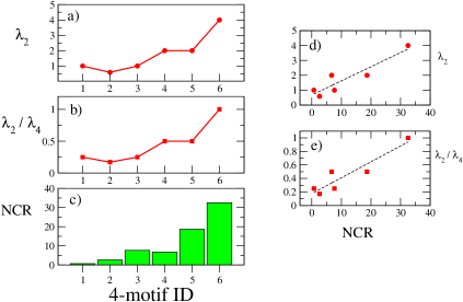
Figure 1: The value of SSS for each of the six 4-node undirected motifs are reported in panel a) for class II systems and in panel b) for class III, and compared with the natural conservation rates (NCR) in the yeast protein interaction network  [18]. The motif identification number is the same as in Ref. [7]. In panel d) and e) we plot the values of SSS as function of the NCR (symbols), and the linear fittings obtained (dashed lines).

We now turn our attention to directed motifs. In a directed graph, the matrix $L$ is asymmetric and in general not always diagonalizable. Nevertheless, $L$ can be transformed into a Jordan canonical form, and it has been proven that the same condition valid for diagonalizable networks ($\Lambda(\sigma\lambda_{k})<0~{}\forall k=2,...,n$) also applies to non-diagonalizable networks [19]. In addition, the spectrum of $L$ is either real or made of pairs of complex conjugates. Because of the zero row-sum condition, $L$ always admits $\lambda_{1}=0$, and the other eigenvalues $\lambda_{k}=\lambda^{R}_{k}+i\lambda^{I}_{k},\ k=2,\ldots,n$ (having non negative real parts according to the Gerschgorin’s circle theorem [20]) can be ordered by increasing real part ($0\leq\lambda^{R}_{2}\leq\ldots\leq\lambda^{R}_{n}$). Consequently, the parametric equation (6) has to be studied for complex values of the parameter $\nu=\nu^{R}+i\nu^{I}$. This yields a master stability function $\Lambda(\nu)$ as a surface over the complex plane $\nu$, that generalizes the plots for the case $\nu$ real. By calling $\cal R$ the region in the complex plane where $\Lambda(\nu)$ provides a negative Lyapunov exponent, the stability condition for the synchronous state is that the set $\{\sigma\lambda_{k},k=2,\ldots,n\}$ be entirely contained in $\cal R$ for a given $\sigma$. This is best accomplished for connection topologies that make ${\lambda^{R}_{2}}$ as large as possible for class I systems, and for topologies that simultaneously make $\frac{\lambda^{R}_{2}}{\lambda^{R}_{N}}$ as large as possible and $\displaystyle\max_{k\geq 2}\{\mid\lambda^{I}_{k}\mid\}$ as small as possible, for class II systems.

In Fig. 2, we consider the thirteen 3-node directed motifs. Two of them, namely motifs #3 and motif #11 give rise to non-diagonalizable $L$. Motif #8 is the only case where the eigenvalues are not real. In the left (right) panels we report $\lambda^{R}_{2}$ for class II systems ($\lambda^{R}_{2}/\lambda^{R}_{3}$ for class III systems).

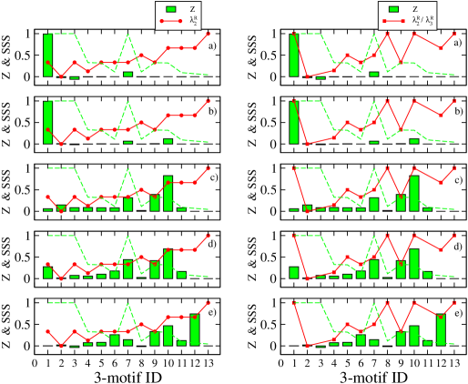
Figure 2: The SSS of each of the thirteen 3-node directed motifs is reported (continuous line) for class II (left panels), and class III systems (right panels). For class III system the SSS values has been normalized to the maximum value so to vary in the range [0,1]. The SSS values are compared with the Z-score (hystograms) and with a measure of the stability of stationary states (dashed line) from Ref.[11], in five different biological networks: the transcriptional regulatory networks of E. coli (panels a) and S. cerevisiae (panel b), the signal transduction knowledge environment (STKE) network (panel c), the developmental transcriptional network of Drosophila melanogaster (panel d), and the neural connection map of C. elegans (panel e).

The SSS measures are compared with the Z-score profile obtained for five different real biological networks, and shown as hystograms in the figure. Both class I and class II systems exhibit an average increase of SSS as a function of the number of links in the motif. However, the overall agreement of the SSS and the Z-score profiles is not as good as in the case of undirected 4-motifs. Here, we have obtained rather small values (ranging from 0.1 to 0.3) of the correlation coefficient, with a better agreement found in the case of the STKE network (panels c), Drosophila (panels d) and C.elegans (panels e), rather than in the transcriptional regulatory networks (panels a and b). This might be due to the fact that synchronization processes are more important in neural systems than in other biological systems as transcriptional networks, especially the simplest ones (E. coli and S. cerevisiae). We have also reported in figure, as dashed lines, the measure of the stability of stationary states proposed by Prill et al. [11]. Such a measure seems to be better indicated for those systems where the stability of stationary states can be a more relevant dynamical quantity to investigate than the stability of synchronous states. Fig. 2 clearly indicates that in some motifs, SSS and Z-score are better correlated than in others. Hence, for each motif $M$, we have defined an overlap coefficient $O_{M}$ as: $O_{M}=SSS_{M}\times Z_{M}$. The maximum possible value $O_{M}=1$ indicates a perfect correlation between SSS and Z-score. The overlap coefficients obtained for the five studied systems are reported in Fig. 3.

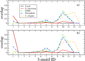
Figure 3: The overlap coefficients for each of the thirteen 3-node directed motifs, and the five biological networks considered, are reported for class II (panel a) and class III systems (panel b).

For both class II and class III systems we have high values of the overlap for motifs: 1, 7, 10, 12.

Finally, we have considered the 199 4-node directed motifs. Here we report the results for three of the most statistically relevant motifs found in biological networks: the bifan, the biparallel and the feedback loop (see Ref. [5]). Such three motifs correspond all to cases in which $L$ can be diagonalized. The biparallel graph, that is abundant in the C. elegans and in transcriptional networks, has real eigenvalues and a relatively high value of SSSs: $\lambda^{R}_{2}=1$ and $\lambda^{R}_{2}/\lambda^{R}_{4}=0.5$. The same is true for the 4-node feedback loop (also found abundant in electric circuits [5]), having $\lambda^{R}_{2}=1$, $\lambda^{R}_{2}/\lambda^{R}_{4}=0.5$ and $\max_{k\geq 2}\{\mid\lambda^{I}_{k}\mid\}=1$. Conversely, the bifan is not compatible with synchronization for any choice of ${\bf F}({\bf x})$ and ${\bf H}({\bf x})$, and for any value of $\sigma$, since $\lambda_{2}=0$ and we have assumed the case of networked chaotic systems ($\Lambda(\nu=0)>0$). In fact, $\lambda^{R}_{2}\neq 0$ iff the graph embeds an oriented spanning tree, (i.e., there is a node from which all other nodes can be reached by following directed links) [21, 19] and this condition, that generalizes the notion of connectedness for undirected graphs [15] to directed graphs, is not valid in the case of the bifan.

We warmly thank R.J. Prill and A. Levchenko for having provided us with their results on the stability of stationary states, and G. Russo for useful comments. S.B. acknowledges the Yeshaya Horowitz Association through the Center for Complexity Science.

References

- [1] R. Albert and A.-L. Barabási, Rev. Mod. Phys. 74, 47 (2002).
- [2] M.E.J. Newman, SIAM Review 45, 167 (2003).
- [3] S. Boccaletti, V. Latora, Y. Moreno, M. Chavez and D.-U. Hwang, Phys. Rep. 424, 175 (2006).
- [4] S. Shen-Orr, R. Milo, S. Mangan and U. Alon, Nature Genetics 31, 64 (2002).
- [5] R. Milo, S. Shen-Orr, S. Itzkovitz, N. Kashan, D. Chklovskii, and U. Alon, Science 298, 824 (2002).
- [6] S. Mangan and U Alon, Proc Natl Acad Sci USA 100, 11980 (2003).
- [7] R. Milo, S. Itzkovitz, N. Kashtan, R. Levitt, S. Shen-Orr, I. Ayzenshtat, M. Sheffer, and U. Alon, Science 303, 1538 (2004).
- [8] N. Kashtan, S. Itzkovitz, R. Milo, and U. Alon, Bioinformatics 20, 1746 (2004).
- [9] S. Valverde and R. V. Solé, Phys. Rev. E72, 026107 (2005).
- [10] A. Vázquez et al., PNAS 101, 17940 (2004).
- [11] R.J. Prill, P.A. Iglesias and A. Levchenko, PLoS Biology 3, 1881 (2005).
- [12] L.M. Pecora and T.L. Carroll, Phys. Rev. Lett. 80, 2109 (1998)
- [13] K.S. Fink, G. Johnson, T.L. Carroll, D. Mar and L.M. Pecora, Phys. Rev. E61, 5080 (2000).
- [14] M. Barahona and L.M. Pecora, Phys. Rev. Lett. 89, 054101 (2002).
- [15] M. Fiedler, Czech. Math. J. 23 (1973) 298.
- [16] D.-U. Hwang et al., Phys. Rev. Lett. 94, 138701 (2005). M. Chavez et al, Phys. Rev. Lett. 94, 218701 (2005).
- [17] Y.Moreno, M. Vázquez-Prada, and A. F. Pacheco, Physica A343, 279 (2004).
- [18] S. Wuchty, Z. N. Oltvai, and A.-L. Barabási, Nat. Genet. 35, 176-179 (2003).
- [19] T. Nishikawa and A. E. Motter, Phys. Rev. E73, 065106R (2006).
- [20] S. A. Gerschgorin, Izv. Akad. Nauk. SSSR, Ser. Mat. 7, 749 (1931).
- [21] C. W. Wu, Linear Algebr. Appl. 402, 207 (2005).