On the reliability of voting processes: the Mexican case

Abstract

Analysis of vote distributions using current tools from statistical physics is of increasing interest. While data considered for physics studies are subject to a careful understanding of error sources, such analysis are almost absent in studies of voting process. As a way to test reliability in electoral processes we choose to investigate the July 2006 presidential election in Mexico. We use records which appeared in the Programa de Resultados Preliminares, PREP, the program which offers electoral results as soon as they are captured. In order to contrast the results we used the congressional election data-set and the July 2000 presidential record. We demonstrate the existence of correlations in the percentage of votes and, we offer evidence of the strong influence of the PRI in the curious results in the presidential case. Distributions of errors in the data-sets are analyzed for all the elections and no large deviations were found. That is, even when the sum of errors is around 45% in all cases, their global behavior is similar. This result gives support to the thesis of no large fraud for the July 2006 presidential election. Distribution of votes in all cases is obtained for all the parties. Parties and candidates with few votes, annulled votes and non-registered candidates follow a power law distribution, and the corporate party follows a daisy model distribution. Parties and candidates with many votes show a mixed behavior.

1 Introduction

Elections are an important matter for humanity. Analysis of how we vote is an important subject in political, social and economical sciences. In recent year, physicists and mathematicians became interested in looking if some of the dynamics and universal behaviors found in statistical mechanics, complex systems and other fields can be used to understand the voting process and the way we form our opinion. Such an area has its own name: sociophysics. The book of Ph. Ball [3] offers a clear and readable introduction to the physicists’ and mathematicians’ incursion in social and economical subjects, meanwhile the report  [9] is a much more technical approach.

In this context, several theoretical models have been successfully applied in order to explain some characteristics on how we take decisions and, in particular, how we vote. However, studies of actual electoral data with the current tools in physics are scarce [5, 6, 7, 8, 13] [17, 21, 24]. The current work is part of an effort to fulfill such an absence and contribute to characterize the statistical properties of actual databases. Certainly, all these approaches are complimentary to the vast literature and studies done in political, social, economical and anthropological sciences.

Here, we are interested in a particular kind of electoral forensics related with the reliability of vote processes. The faithfulness of the data is an important issue, since the record of social processes is subject to all kinds of uncontrollable factors. Furthermore, while data considered for analysis in physics are subject to a careful understanding of the sources of error, such analysis are almost absent in studies of voting process even though election forensics is a current subject in political sciences.

In this work, we present an approach to two problems: we analyze the real time results obtained during the federal election in Mexico in the year of 2006, and we offer an analysis of the distribution of errors obtainable from this public database. Both problems contribute to clarify the dynamics in the Mexican electoral processes, where a misunderstanding of the data give place to suspicious of the existence of a large fraud (Mega-fraud). We present statistical arguments that limit such a suspicious, gives a better perspective of the peculiarities of the Mexican processes where the nonexistence of widespread fraud does not necessarily mean absence of irregularities. We offer, as well, evidence that usual statistical assumptions are not necessarily fulfilled by the electoral processes. The reported forensics in the peer reviewed literature does not consider the tests analyzed here. On the other hand, we do not consider the pre-election events and how they influenced the final result.

We focus the present study on data obtained from the “Program of Preliminary Electoral Results”, or PREP, after its acronym in Spanish [29], which is the system implemented by the electoral authorities (Instituto Federal Electoral, IFE) in order to present the first results as the information arrives to the headquarters. In Mexico, the election is performed using electoral cabins (polling stations) that admit, by construction, around $750$ voters and that are, approximately, uniformly distributed over the population with the right to emit a vote. The PREP works with certificates stamped on the packets of ballots (named electoral packets). In those certificates the citizens who staff polling places write, by hand, the number of votes received for each party, total number of those votes, etc., at the end of the electoral day. Later, the authorities of each electoral cabin deliver the electoral packets and their certificates to the capture centers. The time of arrival is captured as well as the results stamped on the electoral packets. The records are sent to Mexico City headquarters and published on the electoral authorities’ website [25]. The final results are recorded in a public file [29]. The analysis presented here is based on such a file. During the next days IFE admits and discusses objections and appellations. The final results are published in the final count named “Conteo Distrital” or District Count. Disputes about electoral practices are solved by the autonomous Federal Electoral Tribunal. Analysis on statistical aspects of distrital count results are in progress and some have been published [21, 22, 23].

Federal elections in Mexico are performed each six years on the first Sunday of July, including presidential change and renewal of both chambers. For details on how the Mexican electoral systems works see the note of Klesner [27]. An important result is the conformation of the chambers, that depends in a complicated way on the alliances and the relative strength of each political current, see Crespo for an explanation [15].

The political parties who participated in the July 2006 election are grouped in two alliances and several parties. The first party is Partido Acción Nacional (PAN) postulating as candidate to Felipe Calderón Hinojosa (FCH); the first alliance corresponds to Alianza por México composed of the Partido Revolucionario Institucional (PRI) and the Partido Verde Ecologista de México (PVEM), they postulated Roberto Madrazo Pintado (RMP); the second alliance was Alianza por el bien de todos composed of the following political parties: Partido de la Revolución Democrática (PRD), Partido del Trabajo (PT) and Convergencia, with candidate Andrés Manuel López Obrador (AMLO); the last parties are Partido Nueva Alianza with Roberto Campa Cifrián (RCC) and, Partido Alternativa to Patricia Mercado Castro (PMC). The certificates report votes for non registered candidates and annulled votes as well. For the alliances we shall use the main party to identify them, that is we shall call PRI instead of Alianza por México and PRD instead of Alianza por el bien de todos.

The rest of the paper is organized as follows: In the next section, we clarify our lines of argument. We establish the working hypothesis and the alternative one. In section 3, we analyze correlations in the real-time behavior of PREP data. For section 4, we perform an analysis on the six independent self-consistent error distributions that can be build up with the PREP data. As bonus we describe the vote distribution for all the cases in section 5. Conclusions appear in section 6 and some additional information in an appendix.

2 The argumentative line

The Mexican presidential election in 2006 was controversial and suspicions of a large (Mega) fraud has been present since election day. This was at the origin of our interest in analyzing electoral data. However, our lack of expertise in electoral matters shall rule the statistical approach we use. Even when we have experience analyzing statistical properties of complex physical systems, we do not have a clear idea of how a Mega-fraud in elections must looks like. Under this premise, a serious working hypothesis is to depart from the idea that no fraud exists and to perform as many test as we are able, in order to find a qualitative difference in the results of all the cases we shall present.

As pointed out by Good and Harding [18], it is a source of error to “[use] the same set of data to formulate hypothesis and then to test those hypothesis”. Since the data set under suspicion is the presidential election of 2006, we shall contrast all our test with the chambers election of the same year. We complement our results with the analysis of presidential election in Mexico during 2000.

Hence, our working hypothesis is established as:

$H_{1}:$ Data from PREP for the Mexican elections of 2006, presidential and both chambers, present the same qualitative statistical behavior.

The alternative hypothesis is:

$H_{0}:$ Data from PREP for the Mexican elections of 2006, presidential and both chambers, present a qualitative different statistical behavior.

This means, that manipulation in a large scale is present in one of the cases. The meaning of “qualitative difference” will be clear in the section of error distributions. Notice that these hypothesis do not depend on what we expect or not, according to our prejudices. For instance, for physicists it is natural to expect error distributions with a Gaussian or a Lorentzian shape. But, in the present case, we are not dealing with the same objects (particles) or interactions. So, deviations from the canonical, uncorrelated, behavior do not to be assumed as a signature of fraud when appear in different processes.

The philosophy is that before we look what is out of place, we look, first, what is in place. Hence, our study is of a phenomenological nature.

3 Time behavior of PREP

Around $20:00$ hrs on July 2nd, 2006, the Program of Preliminary Electoral Results (PREP) of IFE [29] began to publish on its website the vote percentages for the presidential election of that day. The update was every $5$ minutes and the news services reproduced it. A very close election, according to opinion polls, was expected between the two main candidates of PAN and PRD. (Recall we shall use the names of the main political parties in a coalition). At the beginning, the tendency showed a decrease in the number of votes for the PAN’s candidate and an increase for the candidate of PRD. At first sight, a crossing seemed to be imminent between the percentage of votes obtained by the two candidates. For this reason, several scientists as well as laymen started the capture of real-time data using different methods, some captured by hand, others captured automatically with programs like perl [34, 4].

In Fig. 1(a) we show the plot of the real-time data given by the PREP for the three main candidates captured in election day [4] as well as the data obtained from the PREP file (in lines at the figure). This plot shows roughly two tendencies for the percentage obtained by the candidate of PRD. The increasing tendency changed to a decreasing one around 3:00 AM (around $70\%$ of the processed vote certificates in Fig. 1) of July 3rd. As can be seen in the same figure, the PRI candidate increased its vote percentage changing the tendencies of the candidates of PAN and PRD, respectively.

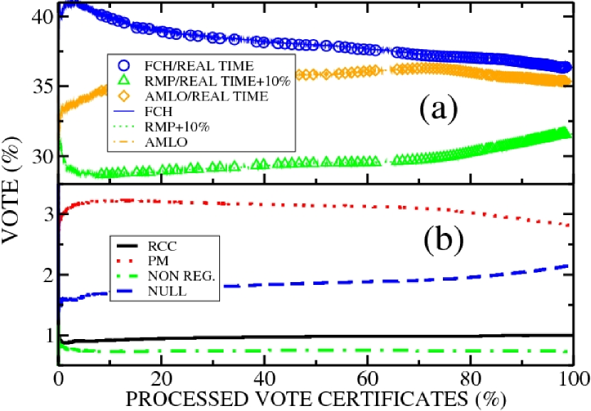
Figure 1: (Color on-line) Real-time data given by the Program of Preliminary Electoral Results (PREP) for (a) the three main presidential candidates and (b) the other two candidates, the votes for non registered candidates and the annulled votes (NULL). The plots in (a) show the percentage of votes obtained per candidate against the percentage of processed vote certificates. The blue circles correspond to Felipe Calderón Hinojosa (FCH), candidate of PAN, the green triangles to Roberto Madrazo Pintado (RMP) for PRI, and the orange diamonds to Andrés Manuel López Obrador for the PRD party. The data were taken from the Internet [34, 4] and correspond to the real time data published by IFE’s web page. We added 10% of votes to RPM in order to show all the results in a smaller window. Notice the change in the slope of this party after the $70\%$ of processed certificates. We show the complete data from the PREP file[29] as well, they are indicated by the corresponding lines. From the same data set we plot, in (b), the percentages obtained for Roberto Campa Cifrián (RCC) for PANAL, Patricia Mercado for Partido Alternativa, we included the vote for non registered candidates (NON REG.) and annulled votes (NULL). Notice that the change in the percentages, for these cases, is small.

As a result, no crossing between the vote percentage of the two main candidates was found with the PREP in real time. In order to test the suspicious that real time data published in the web page of IFE is not coincident with the reported data in the PREP file, we plotted both of them in Figure 1(a), and they agree.

A common belief is to consider that the behavior of a graph like Figure 1 reaches its final value in a direct way, and a change like the presented here looks suspicious. However, one must be careful, since we cannot consider a priori uncorrelated behavior. The graph shows vote percentage and, evidently, this fact introduces correlations between the variables as we shall explain. For the sake of clarity we drop the multiplication by $100$. The percentage of votes for party 1, for instance, at certain time $t$ or percentage of processed vote certificates is calculated by

$$\%V_{1}(t)=\frac{V_{1}(t)}{\sum_{i}^{N}V_{i}(t)},$$ (1)

and for party 2,

$$\%V_{2}(t)=\frac{V_{2}(t)}{\sum_{i}^{N}V_{i}(t)}.$$ (2)

Here $V_{i}(t)$ corresponds to the number of votes received by party $i$ at time $t$. Eliminating the common expression $\sum_{i}^{N}V_{i}(t)$ between both equations we have

$$\%V_{1}(t)=\frac{V_{1}(t)}{V_{2}(t)}\times\%V_{2}(t).$$ (3)

This correlates the percentage $\%V_{1}(t)$ with the precentage $\%V_{2}(t)$, not mattering that the variables $V_{1}(t)$ and $V_{2}(t)$ are random or not. The same is true for the rest of the percentages and for all times. Additionally, the percentage of all the parties must sum $100\%$ as well, hence, it is natural that a “mirror” effect appears in normalized quantities. In Figure 1(b) we show the percentage of vote for the rest of the parties, notice that the values do not present significant changes, hence, the changes are due to the three main parties.

Moreover, the temporal data are not taken from a uniform sample and so we do not expect a fast convergence to the final results. Assuming a clean election, the first data that arrived to the capture centers were from sites with better transport networks and/or a better vote counting performance. In Ref. [37], correlation with an official marginalization index [11] is presented and confirms this assertion: Reports from polling stations inside regions with a low marginalization index arrived early to capture centers. In an earlier version of this paper we presented examples of how the sampling of polling stations rules the shape of the percentage vote graph [2]. Evidently, the final values are the same.

The question that remains is: Does it show some peculiar behavior the number of votes? A way to answer it is to calculate the correlation matrix, and particularly the auto-correlation. In Table 1 we report both, the correlations for percentage of votes in the lower triangular matrix and the correlations for the number votes in the upper triangular matrix. Recall that correlation matrices are symmetric. In the diagonal we report the result of auto-correlations for percentage of votes, the corresponding auto-correlation in number of vote are equal to one in all the cases.

For the lower triangular matrix, the correlation in percentage of votes shows the obvious relation between them, the vast majority is far from zero and near one or minus one. An exception in the case of the presidential candidate of PANAL, RCC, whose auto-correlation is $0.08$(i.e. it is not auto-correlated!). Other anomalies appear with this party and are reported below. Note that not all the auto-correlations in Table 1 are unity, since the percentage and its momenta are calculated prior to calculating each correlation and a large variability in the PREP records exists. These statistics are reported in section 4.

The correlation matrix of percentage of votes for deputies and senators election are presented in the appendix in Tables 3 and 4. The results are similar to those presented in 1: percentage of votes are correlated (or anti-correlated). An interesting point is that PANAL’s percentage of vote auto-correlation is $0.71$ and $0.62$ for deputies and senators, far from the $0.08$ for presidential election.

For the number of votes, as expected, the story is different. The vast majority of correlations reported are close to zero and all the auto-correlations of votes are one. Even the correlation of PANAL with other parties is around zero. The values calculated for the chambers are all consistent with this result: There is no a qualitative difference in the presidential and chambers elections.

A test on the statistical significance of the correlation coefficients can be done using a re-sampling method [19]. However we found much more instructive to show the behavior of the errors in the database. Which is the matter of the next section.

	PAN	PRI	PRD	PANAL	Alter	N.R.	N.V.
PAN	1.00	-0.05	-0.23	0.07	0.35	0.08	-0.06
PRI	-0.77	1.00	-0.15	0.10	-0.17	0.07	0.18
PRD	-0.74	0.15	1.02	-0.02	0.34	0.01	0.00
PANAL	-0.26	0.17	0.22	0.08	0.12	0.07	0.08
Alter	0.70	-0.96	-0.07	-0.16	1.00	0.12	-0.06
N.R.	0.11	0.06	-0.25	-0.03	-0.04	0.82	0.03
N.V.	-0.95	0.81	0.62	0.25	-0.78	-0.19	1.00

Table 1: Correlation matrix of vote percentage, lower triangular matrix, and number of votes, upper triangular, for the presidential election in 2006. Diagonal corresponds to auto-correlation of vote percentage. Notice the anomalous value of the auto-correlation in the PANAL case. N.R. stands for non registered candidates and N.V. for annulled votes.

Returning to the percentage of votes behavior, we analyze the deputies and senators behavior. In Figure  2 we report the equivalent plots of Fig. 1 for the Chambers. In Fig. 2(a) and(c) for deputies meanwhile in (b) and (d) for Senators. The behavior reported for the presidential data is similar in the current case, except that the apparent crossover is not present since the percentages of vote are different. For the 2000 election the behavior is similar and the results for the three main candidates is presented in Fig.  9 at the appendix. It is interesting that a shift (not shown) on the data reproduce the global behavior in the 2006 case, i.e. the growth of the PRI percentage of vote around $70\%$ of vote certificates and the falling of percentage of votes for PRD and PAN before that.

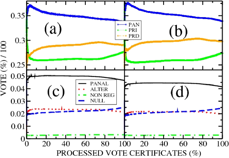
Figure 2: (Color on-line) Same as the previous figure but for election of both chambers. Here the data were obtained from PREP file and we do not have the results published in real time in IFE’s web page. In (a) percentage of votes for the three main parties/coalitions for the deputies election and in (b) for the high chamber. Except for the scales the behavior is similar to the presidential case. A shift (not shown) of the percentage of votes for PAN and PRD for both chambers present the same non-crossing effect as in previous figure. Notice, as well, that PRI have a revival around the $70\%$ of processeed vote certificates in both cases. In (c) and (d) we plot the results for the rest of the parties, non registered and annulled votes for deputies and senators, respectively. Notice that the global behavior in (a) and (b) is similar to figure 1(a). That is: vote for the chambers follows the presidential behavior.

4 Conservation laws in elections

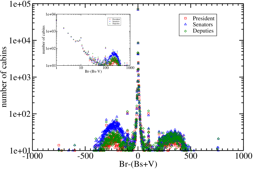
Figure 3: (Color on-line) Error distributions, in logarithmic scale, of the difference between the total ballots received Br and the sum of the remaining ballots Bs and the total number of voters V per cabin, E${}_{1}=$ Br-(Bs+V), for all the cases in July 2006 election. Negative values in the horizontal axis mean more votes than ballots, i.e. there were more voters than documents which certified this fact, and positive values mean appearance of ballots, but in both cases there is no conservation of the total number of received ballots Br per cabin. The inset shows the left branch of the distribution in log-log scale. This shows a power law decay. Note the several sharp peaks in the distribution along the horizontal axis between the values $10$ to $100$. We assume that these peaks are related with typos, but further analysis is required. We note that the distribution for senators show a slightly different behavior in its left branch, compared with the corresponding distributions for president and deputies. The distributions are not normalized.

Another way to test the reliability of the electoral processes is to check the self-consistency of the data-base. In the cabin certificates several data are recorded and several of them must agree. For instance the total number of ballots received the election day must be equal to the number of the remaining ballots plus the used ones. In an ideal election such kind of quantities must give zero for all the cabin records, however we are dealing with an actual process performed by people and some errors could occur, intentional or not. In many processes Gaussian or lorentzian distributions of error appear but in the current case we have no a priori knowledge about the distribution or if the whole amount of votes are enough to reach the limit distribution, if it exists. So, as explained in the argumentative line section, we define and explore the errors that could give us self-consistency in the database and contrast all of them.

The PREP database is composed from the data stamped in the electoral package by the citizens sorted by IFE to conduct the election at the polling station, several of them are easily subject to human error or to intentional alteration and, its distributions must be object of study. The data are: Total number of received ballots at the beginning of the electoral process (Br), number of remaining (not used) ballots (Bs), number of voters (V), number of deposited ballots per cabin (Bd) and the number of votes received for each party/candidate (V_i, $i=$ PAN, PRI, PRD, PANAL, ALTENATIVA, non-registered candidates and annulled votes). The conservation laws that we checked, for self-consistency, are six and they are summarized in table  2.

E1	B. received $-$ (B. not used $+$ Number of voters)	Br - (Bs + V)
E2	B. received $-$ (B. not used $+$ B. deposited)	Br - (Bs + Bd)
E3	B. received $-$ (B. not used $+$ Votes for each party)	Br - (Bs+$\sum_{i}$ Vi)
E4	Number of voters $-$ B. deposited	V - Bd
E5	Number of voters $-$ Votes for each party	V - $\sum_{i}$ Vi
E6	B. deposited $-$ Votes for each party	Bd - $\sum_{i}$ Vi

Table 2: Table of errors considered for a self consistency test of the PREP database. The quantities considered are those that were calculated and registered independently by the electoral authorities (citizens) when the votes were counted. In this sense, they are non-trivial. We use B. as a shorthand for Ballots. The variable $i$ stands for the number of votes obtained for each party/candidate.

The error distribution is build up by calculating the error E_k on each cabin and, then, make the histogram of the values obtained, i.e., how many cabins have values of E_k equal to 0,1,2,$\cdots$. Certainly the values can be negatives as well. In the current work we do not normalize the distributions.

We start the analysis with E₁, that is, the total number of ballots, Br, against the sum of the number of remaining ballots, Bs, and the number of voters per cabin, V, i.e ., E${}_{1}=$ Br-(Bs+V). As seen in Fig. 3, the distribution of E₁ is peaked around zero but is neither the expected Dirac delta function $\delta(x)$, nor a Gaussian nor a Lorentzian. Data on the positive axis mean appearance of ballots, meanwhile data on the negative axis indicate lost of them. In plain English, in the latter case there are more registered people who voted than documents that certified their existence. Zooms in different parts of this distribution show the following facts: (1) The PREP preserve this number for only $\sim 45\%$ of the cabins. This result is unfortunate for the electoral authorities (IFE) since it says that PREP reliability is less than $50\%$. This is even worse since, as we shall see later, the same occurs for the rest of the error distributions considered and in the distributions for both chambers. (2) The distribution is not completely symmetric. In particular the peak around $-250$ is higher than the peak at $250$. (3) There are inconsistencies larger than $750$ votes for several cabins. (4) There are peaks at $\pm 10,\pm 20,\dots$ and also at $\pm 100,\pm 200,\dots$. These peaks, we assume, are related with capture typos, but it is not proved. (5) The peak at the left side of the distribution shows a different behavior for senators than the other cases. (6) The distribution between $1$ and $100$ decays as a power law as can be seen in the insert of figures 3 to 5.

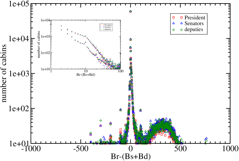
Figure 4: (Color on-line) Error distributions, in logarithmic scale, of the difference between the total ballots received Br minus the sum of the ballots remained Bs plus the ballots deposited in urns Bd by cabin, i.e., E${}_{2}=$ Br-(Bs+Bd). Notice that the asymmetry between the both branches for the three distributions is similar, but it is different from that in previous figure. Again, the left branch of this probability distributions shows the sharp peaks we associated to capture mistakes. The inset shows both branches of the distributions in log-log scale.

In Figs. 4 and 5 we show the distributions of E₂ and E₃ conservation laws. Both distributions should give a delta function $\delta(x)$ in the ideal case. But, as seen in Figure 4, it is very asymmetric and present extreme values around $750$ as in Fig. 3. In the insets we show that typos are also present and that power laws appear. The results for E₄ and E₅ are similar.

In the previous analysis all the cabins were considered, notwithstanding the fact that a selection is required, since many records present alterations as was documented by Crespo [14]. However, statistical analysis, like the present one are valid, since the universal source of error must be studied for future references. Other errors, random or systematic, require future analysis as well.

The result of presidential 2006 election caused a debate about the existence or not of a Mega-fraud against the candidate of PRD and this section offers a new insight into the question. Since the error distributions of all the cases have a similar behavior, we have only two options: i) There was no large fraud in presidential election, or ii) There was a large fraud in all the cases, including both chambers.

In order to differentiate between the previous options we calculated the same error distributions for the PREP corresponding to the presidential election in 2000. We summarize the results in Fig. 6. As can be seen, the main characteristics of whole election in 2006 are present in the 2000 election. Nobody mentioned a fraud or a mega-fraud then, but certainly the present results tell something about the dynamics in Mexican elections. The large amount of errors and vicious practices certainly are present in both elections, and requires of a separate analysis. It is important to remark that it is not only the amount of errors important, the distributions show the dynamics and hopefully an analysis of them will provide us a better understanding of the human processes that an election imply. Aparicio [1] reports that the percentage of errors are similar in the presidential elections in 2000 and 2006, but here we offer new tools to understand such a behavior. For instance, even when the amount of received ballots at each cabin is around 750, the reported quantity present large deviations, many of them, probably, due to carelesnes of the citizen authorities record. If this is of a malicious origin is unclear but opens the opportunity for new analysis. Another point is that performing sums under pressure could be a no trivial matter. Measuring the distribution of such behaviors is an open task to social scientists and suggest the performance of experiments as well. allows to perform experiments as well. For example, to design an experiment to obtain the distribution of typos under pressure in the capture line. To the knowledge of the authors this distribution has not been reported in the literature. The meaning of the lobes with maximum around $\pm 250$ must be analyzed as well as the power law decay in all the studied cases.

As a final remark of this section, we note that with the large amount of errors the result in the presidential election of 2006 could remain unclear and a technical tie. However, analysis similar to the presented here, including the chambers election and comparison with other electoral but equivalent processes, is useful in order to clarify the forensics of fraud or not in future elections, in Mexico or in any democracy.

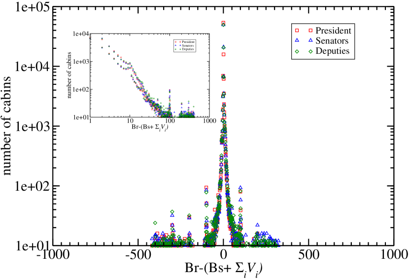
Figure 5: (Color on-line) Error distributions, in logarithmic scale, for the difference between the total ballots received Br minus the sum of the ballots remaining Bs plus the sum of votes obtained by each political party, including null votes $\sum_{i}$ V_i, that is E${}_{3}=$ Br-(Bs+$\sum_{i}$ V_i). The meaning of the right and the left distribution branches is similar to that in figure 3. Notice that the three distributions are similar. The inset shows both branches of the distributions in log-log scale.

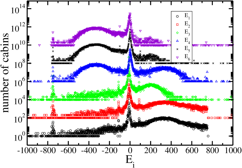
Figure 6: (Color on-line) All error distributions for the presidential election in 2000. The meaning of E_i are reported in Table 2. Date were taken from the corresponding PREP file. In order to see all the cases in the same plot we multiply resulting distribution by a factor of one hundred each time. As seen in the plot the global behavior is similar to those appeared in the whole 2006 electoral process. The scale in $y$-axis is logarithmic.

5 Distribution of the votes

As a final study we deal with the histograms of the number of electoral cabins (polling stations) with a certain number of votes shown in Fig. 7. These histograms are the non normalized vote distribution for each party/candidate. The results for PAN,PRI and PRD presidential candidates appear in Fig. 7(a) and the corresponding results for deputies and senators in panels (b) and (c). Panel (d) of this figure corresponds to PANAL, Alternativa, non-registered candidates and null votes for the presidential election.

Histograms for the votes of PRI change very slowly in the three cases (Fig. 7(a) to (c)). The tail of these distributions looks exponential (a fit is shown in Fig. 8). This is not the case for the distributions of the two main presidential candidates (Fig. 7(a)). The distribution of the votes for FCH/PAN shows a very different behavior for electoral cabins with less than $\sim 40$ votes, since it starts flat. The distribution for AMLO/PRD is also irregular. It shows three different regimes. It appears like a distribution in which realizations between 60 and 300 votes are missing. This could be due to two reasons: the first, is that the data were manipulated; the second, is that the distribution of the votes for PRD is composed of two or more distributions corresponding to several voter dynamics [32]. As an example, a weighted sum of two distributions

$$P=pP_{Daisy}(\langle v_{1}\rangle,\sigma_{1})+(1-p)P_{log-normal}(\langle v_{2}\rangle,\sigma_{2})$$ (4)

with different centroids, $\langle v_{1}\rangle$ and $\langle v_{2}\rangle$, like a Daisy model (see below) and a log-normal distribution could give place to such deformed distributions. Both functions correspond to different groups of voters, the first one to corporate voters  [21] and the other to certain proportional elections [17]. The distributions for the senators and deputies present similar behavior as seen in Fig. 7 (b) and (c). In fact, the participation of a uniform group of voter in important elections is, a priori, unlikely; so, it is enough to have two kind of voters following distribution with different maxima to have such a behavior. This topic is matter of current research by one of us.

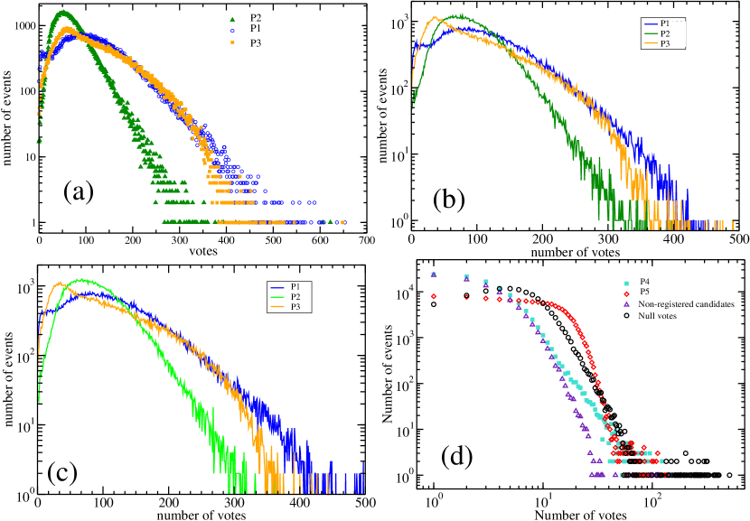
Figure 7: Histograms showing the number of electoral cabins whith given number of votes for the three main parties, (a) president, (b) deputies, (c) senators. In (d) the results votes for president by the small parties are given. Note that the P2 distribution have an exponential tail while the distribution of the small parties show a shifted power-law.

The histograms for the parties with a small number of votes are given in Fig. 7(d). As seen, all histograms have a similar behavior, except for a small numbers of votes. All are shifted power-laws, except for the PANAL presidential candidate which presents deviations. The results for deputies and senators for the same parties are similar (not shown). These results can be explained with several models of cluster growth in complex networks [13, 17], for instance, and appear in other electoral processes [12, 24] for proportional votes. All these stidies are in search of a universal dynamics in voting processes. A research along these lines for the Mexican elections is in progress. We found an inconsistency in the tail of the annulled votes. This distribution shows several electoral cabins with more than 100 annulled votes. The probability of having such results is negligible, so that these results are not statistical, i.e., they are the result of negligence or of a malicious act.

Finally, we return to the PRI case. The distribution of votes for this party is clearly smooth and a fit using the so called Daisy models [20] was performed previously on the final records (Distrital count) for Mexican elections in 2000, 2003 and 2006 [21]. The corresponding fit for the presidential PREP data corresponds to a rank $r=3$ model

$$P_{3}(s)=\frac{4^{4}}{3!}s^{3}\exp(-4s),$$ (5)

for the distribution’s central part, and an $r=2$ model

$$P_{2}(s)=\frac{3^{3}}{2!}s^{2}\exp(-3s),$$ (6)

for the tail. A plot on the normalized distribution of votes appears in Figure 8. Here the “unfolding” of votes is performed using a $4$th degree polynomial on windows of $300$ and $3000$ cabin certificates obtaining a reliable average density of events . Notice that no fitting parameter was used, in contrast to a Brody or a Weibull distributions. The reason of this behavior is unclear and requires a local analysis of the distribution in order to separate the states and municipalities ruled traditionally by PRI. A connection with a geographical approach could be of interest [38]

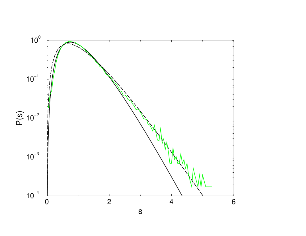
Figure 8: Unfolded distribution for a randomly shuffled sequence of votes for the P2 presidential candidate (green line). A daisy model of rank $r=2$ and $3$ (see text for details) are shown in dashed and continuous black lines.

6 Conclusions

We studied some statistical properties of the federal Mexican elections using the Program of Preliminary Electoral Results (PREP) database from 2000 and 2006. Our main goal was to test reliability in electoral processes, mainly in a controversial election where people suspect of a Mega-fraud. Since we do not have previous experience in electoral data and we do not know how specifically a Mega-fraud must look we chose to test the hypothesis:

$H_{1}:$ Data from PREP for the Mexican elections of 2006, presidential and both chambers, present the same qualitative statistical behavior.

And the alternative one:

$H_{0}:$ Data from PREP for the Mexican elections of 2006, presidential and both chambers, present a qualitative different statistical behavior.

We did tried our best effort to test these hypothesis.

The first suspicion of cheating behavior was the non crossing between the vote percentage of AMLO and FCH in the real time data. We demonstrate that the percentage of votes are correlated while the number of votes are not. The change in slope is strongly altered by the PRI increase of the number of votes around the $70\%$ of the processed vote certificates. This behaviour is reproduced in both chambers election of the same year and in the presidential election in 2000. This contradicts hypothesis H₀ for the time behavior.

A second test concerns the self consistency of the data-set that appears in the PREP file. For an ideal case the sum of votes for all party/candidates and the remaining ballots must be equal to the number of ballots received at the poll station in the election day, for instance. From the set of data in the file six different and independent test of self consistency can be constructed (see 2 ). All of them can be subject of error, from a honest human mistake to a cheating alteration in many of the known ways. Hence we built up the error distribution, which consist of the histogram of the selected error for all the cabins records. We found a similar global behavior in all the cases, for the presidential election in 2006, which is under suspicion of fraud, for both chambers election in the same year and, in the presidential election in 2000. The later was assumed as a clean or at least not disputed election for the participants. In all the cases, the error distributions have a central peak with a power law decay in, approximately, the interval from $-50$ to $50$. All of them have a lobe around $\pm 300$ or $\pm 400$, but generally asymmetric. Some revivals or peaks in $\pm 10$, $\pm 20$,$\dots$, appear in the 2006 cases and they are less prominent in the presidential election of 2000. We suspect of typos for this kind of errors, but, as all the characteristics presented in the current paper, these must be tested with experiments and with new evidence. For instance, at our best knowledge, there is no distribution of typos under pressure conditions. Hence for the self consistency test no large deviations were observed and, H₁ is confirmed.

Even with the evidence provided here and in the peer reviwed literature it is possible the existence of a large fraud, but the probability of such a case is small. Clarification of July 2006 presidential election in Mexico is of a historical importance and hence requiere of more analysis. What we consider much more interesting at this is to insist that electoral processes are subject to a lot of errors and comparisons with theoretical models and predictions must take this fact in to account. We offered, that is our hope, new ways to tipify errors. It is not enough to talk about the magnitude of the errors, since a dynamics inside exists. We leave to an ulterior work comments on the way the cheating could appear in the error distributions. For instance, another explanation for the peaks in such a distributions is that the party representative altered the vote record by adding a zero to the total votes obtained by their own party, transforming a $7$ into $70$, for instance. Or how the errors are distributed along the maginalization index?. Are they distributed in the same way or are different?. How to the different and well know malicious behaviour apperars in these distributions?

As a final remark, we also have obtained the distributions of votes for the different parties. In particular, the distribution of the party that was in power in Mexico during more than $70$ years behaves smoothly. Daisy models of 2nd and 3rd rank seem to fit different parts of the measured distribution. In contrast, the distributions of the parties with more votes are more complex and, probably, composed of different voters dynamics. Distributions of small parties follow power laws. This behavior is consistent with several theoretical models.

7 Acknowledgments

This work was supported by DGAPA-UNAM, PROMEP/SEP and projects UAM-A CBI. We thank C. Badillo for useful comments. We wish also thank E. Morfín for his invaluable help with the database of the PREP, and A. Baqueiro for allowing us the use of real-time captured data of the PREP for Fig. 1.

8 Appendix: Additional data

In this appendix we present additional data, required for comparison. In tables 3 and 4 appear the correlations for percentage of vote (lower matrix) and for number of votes (upper matrix). The correlations were calculated using the standard method

$$c(x,y)=\frac{1}{N}\sum^{N}_{i}\hat{x}(i)\hat{y}(i),$$ (7)

where

$$\hat{x}(i)=(x(i)-\bar{x})/\sqrt{Var(x)},$$ (8)

for the corresponding variable, the number of votes or the percentage of them, for all the combinations of political parties.

In Figure 9 the time behaviour of PREP file during July 2000 is shown.In this case, the PRI appears in second place, but with a change in its slope around $70\%$ of polling stations processed. Shifting these percentages in order to show them as in july 2000 presidential election resembles the same bahavior. The shifting is not shown. Notice that in this figure as well as in all in the paper consider all the data available.

	PAN	PRI	PRD	PANAL	Alter	N.R.	N.V.
PAN	1.00	0.06	-0.3	0.22	0.22	0.00	-0.04
PRI	-0.45	1.02	-0.19	0.02	-0.18	0.00	0.13
PRD	-0.82	-0.16	1.02	0.18	0.41	0.05	0.03
PANAL	0.42	-0.76	0.01	0.71	0.36	0.05	0.02
ALTER	0.48	-0.97	0.08	0.79	1.00	0.06	-0.02
N.R.	-0.84	0.22	0.78	-0.26	-0.27	0.90	0.02
N.V.	0.91	0.42	0.72	-0.52	-0.51	0.81	1.00

Table 3: Correlation matrix of vote percentage, lower triangle, and number of votes, upper triangle, for the deputies election in 2006. Diagonal corresponds to auto-correlation of vote percentage. N.R. stands for non registered candidates and N.V. for annulled votes.

	PAN	PRI	PRD	PANAL	Alter	I.C.	N.V.
PAN	1.00	0.08	-0.31	0.20	0.21	0.01	-0.05
PRI	-0.62	1.02	-0.22	-0.03	-0.19	-0.00	0.12
PRD	-0.83	0.06	1.02	0.28	0.40	0.02	0.03
PANAL	0.28	-0.71	0.14	0.62	0.45	0.06	0.00
ALTER	0.22	-0.86	0.34	0.73	1.00	0.06	-0.02
I.C.	-0.50	0.49	0.27	-0.32	-0.38	0.76	0.02
N.V.	-0.93	0.62	0.73	-0.36	-0.32	0.53	1.00

Table 4: Correlation matrix of vote percentage, lower triangle, and number of votes, upper triangle, for senatorial election in 2006. Diagonal corresponds to auto-correlation of vote percentage. N.R. stands for non registered candidate s and N.V. for annulled votes.

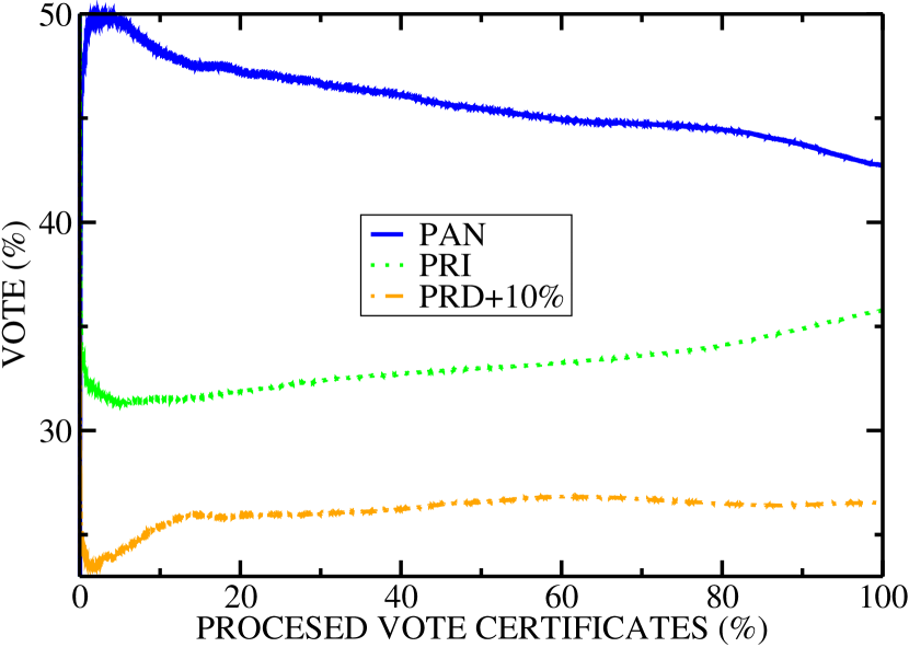
Figure 9: (Color on-line) Percentage of votes as a function of processed vote certificates for the July 2000 presidential election. We use the PREP data and only the three main candidates are shown. Notice the slope change for PRI candidate around $70\%$ of processed vote certificates.

References

- Aparicio, [2006] J. Aparicio. Nexos. Num. 346, Mexico.(2006)
- Báez et al, [2006] G. Báez, H. Hernández-Saldaña and R.A. Méndez-Sánchez. Previous versions of this work. arXiv:physics/0609144 versions 1 and 2.
- Ball, [2004] Ph. Ball, Critical mass: How one thing leads to Another. England. Farrar, Straus and Giroux; 1st edition (June 1, 2004).
- Baqueiro, [2006] Baqueiro, A. private communication.
- Borghesi et al, [2006] Borghesi C, Galam S. Phys. Rev. E 73 (6) (2006) 066118.
- Borghesi et al, [2010] Borghesi C., J-P. Bouchaud. Eur. Phys. J. B. 75 (2010) 395-404
- [7] C. Borghesi, J.C. Raynal and J.P. Bouchaud. Election turnout in many countries: similarities, differences, and a diffusive field model for decision making. arxiv:1201.0524v1 Jan 2, 2012
- [8] Christian Borghesi, Jean Chiche, Jean-Pierre Nadal. “Between order and disorder: a ’weak law’ on recent electoral behavior among urban voters? ” arXiv:1202.6307v1 [physics.soc-ph]
- Castellano et al, [2009] Castellano, Claudio, Fortunato, S., Loreto, V. Statistical physics of social dynamics. Rev. Mod. Phys. 81 (2009) 591-646.
- CD, [2006] Final official results consist of all the vote certificates considered as valid after contests from the parties. This is a different record and appears under the name of Conteo Distrital. This file is public and available at IFE’s website or on request.
- CONAPO, [2005] CONAPO, 2005. Índice de marginación por localidad. 2005@www.conapo.gob.mx
- Costa Filho et al, [1999] R.N. Costa Filho et al Phys. Rev E. 60, 1067 (1999); Physica A 322 (2003) 698.
- Costa Filho et al, [2006] A.A. Moreira, D.R. Paula, R.N. Costa Filho and J.S. Andrade Jr., Phys. Rev E. 73 (2006) 065101(R).
- Crespo, [2008] J.A. Crespo. 2006: Hablan las actas. Las debilidades de la autoridad electoral mexicana.(Debate, 2008). In Spanish.
- Crespo, [2011] Crespo, J.A., 2011. Gobernabilidad y mayorías artificiales. El Universal, October 25.
- Eisenstadt et al, [2006] . Eisenstadt and A. Poiré. Explaining the Credibility Gap in Mexico’s 2006 Presidential Election, Despite Strong (Albeit perfectible) Electoral Institutions. Work Handbook. American University Center for North American Studies.(2006)
- Fortunato et al, [2007] S. Fortunato and C. Castellano, Phys. Rev. Lett. 99 (2007) 138701.
- Good, [2004] P.I. Good and J. W. Harding. Common Errors in statistics and how to avoid them. Wiley; 3 edition (July 7, 2009)
- Good, [2005] P.I. Good. Introduction to statistics through re-sampling methods and R/S-PLUS.( Wiley, 2005)
- Hernández et al, [1999] H. Hernández-Saldaña, J. Flores and T.H. Seligman. Phys. Rev E. 60 (1999) 449.
- Hernández, [2009] H. Hernández-Saldaña. Physica A 388 (2009) 2699. arXiv/physics:0810.0554.
- Hernández, [2010] H. Hernández-Saldaña. Chapter 16. Traveling Salesman Problem, Theory and Applications. D. Davendra (Ed.) InTech. 2010.
- Hernández, [2011] H. Hernández-Saldaña. M. Gómez Quesada and E. Hernández Zapata. Statistical distributions of quasi-optimal paths in the traveling salesman problem: The role of initial distribution of cities. Accepted in Rev. Mex. Fís. S. Available at arXiv/physics:1003.3913v2 [cond.-math.stat-mech] 2011.
- Herrmann et al, [2004] M.C. Gonzalez, A.O. Sousa, and H.J. Herrmann, Int. J. Mod. Phys. C 15 (2004) 45.
- http://www.ife.org.mx, [2006] http://www.ife.org.mx
- Jiao et al., [2006] Jiao Y, Syau YR, Lee ES. Mathematical and Computer Modeling 43 (3-4) (2006) 244-253.
- Klesner, [2007] Klesner, J.L., 2007. The July 2006 presidential and congressional elections in Mexico, Electoral Studies 26 803-808.
- Lang, [2005] Lang J. Proceedings Lecture Notes in Computer Science 3571 (2005) 15-26.
- PREP, [2006] All data were obtained form the web page of the IFE, http://www.ife.org.mx/prep2006/bd_prep2006/bd_prep2006.htm
- Mantovani et al, [2011] M. C. Mantovani, H. V. Ribeiro, M. V. Moro, S. Picoli Jr. and R. S. Mendes Scaling laws and universality in the choice of election candidates. Euro Physics Letters, 96 (2011) 48001. http://arxiv.org/pdf/1109.4360 (2011)
- Mebane, [2006] Mebane, W.,Jr, 2006.Election Forensics: Vote Counts and Benford’s Law Working Paper, Political Sciences Department, Michigan University.
- Merlin et al, [2004] Merlin V, Valognes F. Mathematical Social Sciences 48 (3) (2004) 343-361.
- Miller, [2004] Miller C.A., Social Studies of Science 34 (4) (2004) 501-530.
- Mochan, [2006] http://em.fis.unam.mx/public/mochan/elecciones/indexen.html.
- Moreno, [1998] Moreno, A., 1998. Party competition and the issue of democracy: ideological space in Mexican elections. In: Serrano, M. (Ed.), Governing Mexico: Political Parties and Elections. Institute of Latin American Studies, London.
- Moreno et al, [2007] Moreno, A., Méndez, P., 2007. La identificación partidista en las elecciones presidenciales de 2000 y 2006 en México: ¿Desalineación o realineación? Política y Gobierno, 14.
- Pliego, [2007] F. Pliego Carrasco. El mito del fraude electoral en México. (Pax México, 2007). In Spanish.
- Suárez et al, [2011] Suárez, M., Alberro, I. Electoral Studies 30 136-147.