Elastic turbulence in von Karman swirling flow between two disks.

Abstract

We discuss the role of elastic stress in the statistical properties of elastic turbulence, realized by the flow of a polymer solution between two disks. The dynamics of the elastic stress are analogous to those of a small scale fast dynamo in magnetohydrodynamics, and to those of the turbulent advection of a passive scalar in the Batchelor regime. Both systems are theoretically studied in literature, and this analogy is exploited to explain the statistical properties, the flow structure, and the scaling observed experimentally. The following features of elastic turbulence are confirmed experimentally and presented in this paper:
(i) the rms of the vorticity (and that of velocity gradients) saturates in the bulk of the elastic turbulent flow, leading to the saturation of the elastic stress.
(ii) the rms of the velocity gradients (and thus the elastic stress) grows linearly with $Wi$ in the boundary layer, near the driving disk. The rms of the velocity gradients in the boundary layer is one to two orders of magnitude larger than in the bulk.
(iii) the PDFs of the injected power at either constant angular speed or torque show skewness and exponential tails, which both indicate intermittent statistical behavior. Also the PDFs of the normalized accelerations, which can be related to the statistics of velocity gradients via the Taylor hypothesis, exhibit well-pronounced exponential tails.
(iv) a new length scale, i.e the thickness of the boundary layer, as measured from the profile of the rms of the velocity gradient, is found to be relevant for the boundary layer of the elastic stresses. The velocity boundary layer just reflects some of the features of the boundary layer of the elastic stresses (rms of the velocity gradients). This measured length scale is much smaller than the vessel size.
(v) the scaling of the structure functions of the vorticity, velocity gradients, and injected power is found to be the same as that of a passive scalar advected by an elastic turbulent velocity field.

I Introduction

Long polymer molecules added to a fluid make it elastic and capable to store stresses that depend on the history of deformation, thereby giving the medium a memory bird . As was recently demonstrated, elastic stress can overcome the dissipation caused by relaxating polymer molecules, and can cause complicated and irregular motion in curvilinear shear flows Nat ; NJP . The discovery of elastic turbulence, a random flow in dilute polymer solutions at arbitrary low Reynolds numbers, $Re$, calls for quantitative studies of all aspects of the phenomenon, both experimentally and theoretically.

Although the notion of turbulence itself is widely used in scientific and technical literature, there is no commonly accepted definition. Turbulent flow is usually identified by its main features. Turbulence implies fluid motion in a broad range of temporal and spatial scales, so that many degrees of freedom are excited in the system. There are no intrinsic characteristic scales of time and space in the flow, except for those restricting the excited temporal and spatial domains from above and below. Turbulent flow is also usually accompanied by a significant increase in momentum and mass transfer. That is, flow resistance and rate of mixing in a turbulent flow become much higher than those would be in an imaginary laminar flow with the same Reynolds number.

Random flows of dilute polymer solutions too, cause a sharp growth in flow resistance, exhibit an algebraic decay of velocity power spectra over a wide range of scales, and provide a way for effective mixing Nat ; NJP ; mix . These properties are analogous to those of hydrodynamic turbulence. Such formal similarities give a reason for calling such flows "elastic turbulence". However, the similarities do not imply that the physical mechanism that underlies the two kinds of random motion is the same. Indeed, in contrast with inertial turbulence at high $Re$, which occurs due to large Reynolds stresses landau , large elastic stress is the main source of non-linearity and the cause of elastic turbulence in low $Re$ flows of polymer solutions stretch . One can suggest that in a random flow driven by elasticity, the elastic stress tensor $\bm{\tau}_{p}$ should be the object of primary importance and interest, and that it may be appropriate to view elastic turbulence as turbulence of the $\bm{\tau}_{p}$ field. It would then be more relevant and instructive to explore the spatial structure and the temporal distribution of this field, but, unfortunately, currently no experimental technique allows a direct local measurement of it in a turbulent flow. On the other hand, properties of the $\bm{\tau}_{p}$ field in a boundary layer can be inferred from measurements of injected power, whereas its local properties can be evaluated from measurements of spatial and temporal distributions of velocity gradients.

In this regard, we would like to point out the deep similarity between elastic turbulence and the small-scale turbulent magneto-dynamo discussed theoretically by Volodya2 , that will be further clarified in the next Section. Both the small-scale magneto-dynamo schekochihin as well as elastic turbulence arise when the flow is three-dimensional, random in time and spatially smooth. Analogously to elastic turbulence, the small-scale magneto-dynamo exhibits a viscosity-dominated, low $Re$ turbulence that is much faster than the large-scale one. The small-scale turbulent dynamo is produced by the random stretching of nearly frozen-in magnetic field lines by the ambient velocity field, which is random and spatially smooth, with a growth rate of the order of the inverse viscous eddy-turnover time. The stretching of the magnetic field amplifies exponentially the field strength, at the rate of turbulent stretching, and produces dynamically significant fields before the large-scale fields can grow appreciably schekochihin . The advection of the field then spreads the magnetic energy over a sub-viscous range of scales and piles it up at the resistive scale. Below that scale, diffusion dominates and causes an exponential decay of the energy. This fast dynamo mechanism, due to stretching and folding, generates magnetic field lines which remain straight and fairly well-aligned. Similarly, passive scalar mixing in the Batchelor regime gives rise to the so-called collinear anomaly chertkov95 (see further for details). The fundamental difference between the fast small-scale magneto-dynamo and the elastic turbulence lies in what happens when the small-scale magnetic field becomes sufficiently strong for the Lorentz force to react back on the flow. The different dissipation mechanism in the two systems leads to a different saturation mechanism. In the latter system, saturation is reached when the dynamo stretching that produces the feedback on the velocity field and the homogeneous linear damping balance, whereas this balance is missing in the former case.

The microscopic phenomenon responsible for the macroscopic elastic turbulent flow of dilute polymer solutions is the so-called coil-stretch transition, discussed originally by Lumley lumley and then elaborated by de Gennes deGennes . The essence of the coil-stretch transition is as follows: all the polymer molecules are normally, in absence of a flow gradient, coiled into compact and nearly spherical tangles with radii much smaller than the total polymer length. In the presence of random flow gradients, the polymer molecules are deformed into ellipsoid-like tangles. The mean deformation is moderate as long as the stretching rate of the flow is smaller than the inverse polymer relaxation time. When the stretching rate exceeds the inverse polymer relaxation time, most of the molecules are strongly stretched to sizes up to the order of the total polymer length, since stretching is limited only by non-linear effects and back reaction of the flow. There is an abrupt change in the polymer conformation occurring at large stretching rates, called the coil-stretch transition. The transition has remarkable macroscopic consequences. While in the coiled state the influence of polymers on the flow is negligible and the polymer solutions can be treated as Newtonian fluids (without memory), in the stretched state polymers produce an essential feedback on the flow, and the properties of the solution become strongly non-Newtonian. Let us stress that the coil-stretch transition can occur even at small Reynolds numbers or at low level of hydrodynamic nonlinearity. The elasticity of the polymers itself (which manifests itself above the coil-stretch transition) is a source of nonlinearity. This explains how a chaotic state, which requires a high level of nonlinearity, can arise even at low $Re$ in elastic turbulence.

Another important characteristic of the elastic turbulence regime to be investigated is the scaling of the velocity field. The power spectrum of velocity fluctuations measured in the experiments Nat ; NJP shows a power-law behavior $f^{-\delta}$ with $\delta>3$, where $f$ is the frequency. Since the power spectrum decays strongly with the frequency (and thus with the wave number), the fluctuations of the velocity and of the velocity gradients are both determined by the integral scale, i.e. the size of the vessel. This explains why elastic turbulence is essentially a smooth random flow, dominated by the strong nonlinear interaction of few large-scale modes. A theoretical explanation of the power velocity spectrum was provided by Fouxon and Lebedev Volodya ; Volodya2 . The spectrum $k^{-\delta}$ with $\delta>3$ implies that elastic turbulence flow can be assimilated to a Batchelor regime flow, i.e. a temporally random and spatially smooth flow taylorhypoth . This type of a random flow appears in hydrodynamic turbulence below the dissipation scale.

In a spatially smooth flow, velocity differences are proportional to distances between two fluid particles. As a result, particles separate or approach exponentially in time. The statistics of stretching and contraction of the fluid element can be described by the formalism of dynamical systems, using the notion of Lyapunov exponents that are the exponential rates of divergence. The number of the Lyapunov exponents is equal to space dimensionality, and they are ordered in such a way that the first Lyapunov exponent is the largest and describes the separation rate of two fluid particles. Based on the Lagrangian approach, the so-called collinear anomaly was predicted (first, within the Kraichnan model and then for the general case): a spatially smooth flow locally preserves straight lines chertkov95 . This anomaly, translated into the spatial distribution of the passive scalar, suggests that parallel strips are the major structural elements in the Batchelor regime. The collinear anomaly is also the source of strong intermittency and of the absence of scale invariance observed at scales larger than the forcing scale chertkov95 . This simple yet fundamental feature was observed experimentally for a passive scalar in elastic turbulence mix ; Nat ; Teo .

Such a Batchelor flow is therefore an efficient mixer due to the exponential divergence of Lagrangian trajectories. This property was directly confirmed experimentally in curvilinear channel flows of polymer solutions, where elastic turbulence was excited mix ; Teo . The passive scalar (dye) mixing had there an exponential character along the channel. Additionally, the Lagrangian technique was used (a) to predict the exponential tails of the passive scalar distribution function in the steady regime, as was later confirmed experimentally and numerically; (b) to account for a complex interplay between Lagrangian stretching and diffusion, thus showing that the PDF of the scalar dissipation field has a stretched-exponential tail falkovich ; (c) to explain strong intermittency in the scalar decay problem son ; fouxon , where the decay rate is exponential in time and the exponent saturates to a constant for high-order moments. While the experiment mix confirmed the exponent saturation, it contradicted some other conclusions of the theory developed for infinite domains son ; fouxon . This observation motivated theorists to develop a new (and much-needed) theory of mixing in finite vessels chertkov2 . This theory explained that long-time properties of scalar decay are determined by the stagnation regions of the flow, in particular boundary layers. A nontrivial dependence of the decay rate on diffusivity was predicted, as remarkably confirmed by the experiment on mixing in elastic turbulence Teo . These experimental discoveries and subsequent theoretical developments show the need to readjust the thinking in fundamental fluid mechanics (that mixing of highly viscous fluids is difficult) but also open up a whole new world of practical applications.

Elastic turbulence gives the possibility to dramatically increase mixing rates (and, correspondingly, rates of chemical reactions) of polymer melts in industrial reactors and in small-scale flows (via capillaries, for instance). Indeed, to mix fluids effectively one needs irregular motion, which brings into near contact distant portions of the fluids. This method of mixing begins to find applications in microfluidics and biophysics patent . It is likely that Nature itself uses the trick of small-scale mixing by elastic turbulence. Biological discoveries and applications along this direction are likely to follow.

In this paper we present experimental results concerning statistics of the injected power and statistics and structure of the velocity field in an elastic turbulent flow, in its bulk as well as near a wall. By using the analogy between passive scalar advection in the Batchelor regime and advection of elastic stresses in elastic turbulence, we try to elucidate the role of the latter, particularly in connection with the intermittency and skewness of the injected power statistics, with the statistics and saturation of rms of vorticity (velocity gradients) in the bulk, and with various properties of the velocity profile in the elastic turbulent flow regime, such as scaling and properties of the boundary layer.

Our experimental program addresses the following questions:

(i)

Does elastic stress saturate in the bulk as predicted theoretically, and what is the saturation value?

(ii)

What is the mechanism for pumping energy from the driven plate into the bulk?

(iii)

What is the probability distribution of the elastic stresses?

(iv)

What is the velocity profile in the cell, and does an analog of a boundary layer exist?

(v)

If the boundary layer exists, which length scale characterizes its thickness, and what is the nature of this scale?

(vi)

Are there similarities in the statistical and scaling behavior with the problem of turbulent advection of a passive scalar?

The paper is organized as follows. We start the next section presenting a hydrodynamic description of dilute polymer solution flows and derive non-dimensional parameters to characterize the flows that follow from the equations. The variation of one of these control parameters, responsible for the elastic properties of a fluid, can lead to elastic instability in the swirling flow between two disks, distinguished by the presence of curvilinear trajectories. The stretching of polymer molecules, leading eventually to the coil-stretch transition, is further discussed in section II.2. The theoretical criterion for the elastic instability in different flows, together with its experimental verification, are discussed in section II.3. How this instability is responsible for the scenario dubbed elastic turbulence is addressed in section II.4. The experimental measurement techniques used to characterize the flow are presented in section III.1, and to complete the basics, the rheometric properties of polymer solutions used are given in section III.2, while previous experimental observations of elastic instability in the von Karman flow are summarized in section III.3 and compared to our findings. In section IV we give a complete account of the results of the measurements. Different aspects of the flow are investigated with different techniques: we concentrate on the statistics of global power fluctuations in section IV.1; on the topology of the flow below and above transition and its relation with the observed statistics in IV.2; on profiles of velocity and velocity gradients, and the emergence of boundary layers in section IV.3. All the new experimental facts are summarized and discussed in in section IV.4, where the role of elastic stress, a recent theory of elastic turbulence, and comparative considerations about elastic versus hydrodynamic turbulence are made. Finally, in section V the results are summarized and conclusions are drawn.

II Hydrodynamical theory of elastic turbulence

II.1 Hydrodynamical description of dilute polymer solution flows

Solutions of flexible high molecular weight polymers are viscoelastic liquids, and differ from Newtonian fluids in many aspects bird . The most striking elastic property of polymer solutions is, probably, the dependence of mechanical stresses on the history of the flow. The stresses do not immediately become zero when the fluid motion stops, but rather decay with some characteristic relaxation time, $\lambda$, which can be well above a second. When a polymer solution is sufficiently diluted, its stress tensor $\bm{\tau}$ can be divided into two parts, $\bm{\tau}=\bm{\tau}_{s}+\bm{\tau}_{p}$. The first term, $\bm{\tau}_{s}$, is defined by the viscosity of the Newtonian solvent $\eta_{s}$ and by the rate of strain in the flow, $\bm{\tau}_{s}=\eta_{s}[\mathbf{\nabla}\cdot\mathbf{V}+(\mathbf{\nabla}\cdot\mathbf{V})^{T}]$. The elastic stress tensor, $\bm{\tau}_{p}$, is due to the polymer molecules, which are stretched in the flow, and depends on the history of the flow. The equation of motion for a dilute polymer solution has the form bird

$$\frac{\partial\mathbf{V}}{\partial t}+(\mathbf{V\cdot\nabla)V}=-\frac{\mathbf{\nabla}p}{\rho}+\left(\frac{\eta_{s}}{\rho}\right)\mathbf{\nabla}^{2}\mathbf{V}+\frac{\nabla\cdot\bm{\tau}_{s}}{\rho}\,\,,$$ (1)

where $p$ is the pressure and $\rho$ is the density of the fluid. One can see that $\bm{\tau}_{p}$ enters the equation of motion linearly. The equation has a non-linear term, $(\mathbf{V\cdot\nabla)V}$, which is inertial in its nature. The Reynolds number $Re$ defines the ratio of this non-linear term to the viscous dissipative term, $\nu\mathbf{\nabla}^{2}\mathbf{V}$. Therefore the degree of non-linearity of the equation of motion can still be defined, even for a polymer solution, by the Reynolds number, $Re=VL\rho/\eta_{s}$. Turbulence in fluids at high $Re$ is a paradigm for strongly nonlinear phenomena in spatially extended systems landau ; Tritt .

The simplest model incorporating the elastic nature of the polymer stress tensor, $\bm{\tau}_{p}$, is a Maxwell type constitutive equation bird with a single relaxation time, $\lambda$,

$$\mathbf{\bm{\tau}}_{p}+\lambda{\frac{D\bm{\tau}_{p}}{Dt}}=\eta_{p}[\mathbf{\nabla\mathnormal{\mathnormal{\cdot}}{V}+\mathnormal{(}\nabla\mathnormal{\cdot}{V}\mathnormal{)}^{\mathnormal{T}}}]\,\,.$$ (2)

Here $D\bm{\tau}_{p}/Dt$ is the material time derivative of the polymer stress, and $\eta_{p}=\eta-\eta_{s}$ is the polymer contribution to the total viscosity $\eta$. An appropriate expression for the time derivative $D\bm{\tau}_{p}/Dt$ has to take into account that the stress is carried by fluid elements, which move, rotate and deform in the flow. The translational motion implies an advection term $(\mathbf{V}\cdot\mathbf{\nabla})\bm{\tau}_{p}$, while the rotation and deformation of the fluid particles leads to contributions like $(\mathbf{\nabla}\cdot\mathbf{V})\bm{\tau}_{p}$ or $\bm{\tau}_{p}(\mathbf{\nabla}\cdot\mathbf{V})$ bird . Therefore, some nonlinear terms, in which $\bm{\tau}_{p}$ is coupled to $\mathbf{V}$, appear in the constitutive relation along with terms linear in them. A simple model equation for $D\bm{\tau}_{p}/Dt$, which is commonly used for description of dilute polymer solutions, is the upper convected time derivative,

$$\frac{D\bm{\tau}_{p}}{Dt}=\frac{\partial\bm{\tau}_{p}}{\partial t}+(\mathbf{V}\cdot\mathbf{\nabla})\bm{\tau}_{p}-\bm{\tau}_{p}(\mathbf{V}\cdot\mathbf{\nabla})-(\mathbf{\nabla}\cdot\mathbf{V})^{T}\bm{\tau}_{p}\,\,.$$ (3)

The equations (2,3) together with the expression for $\bm{\tau}_{s}$ constitute the Oldroyd-B rheological model of polymer solutions bird . One can see that the nonlinear terms in the constitutive equation (Eqs. (2,3)) are all of the order $\lambda(V/L)\tau_{p}$. The ratio of those non-linear terms to the linear relaxation term, $\bm{\tau}_{p}$, that represents dissipation, is given by a dimensionless expression $\lambda(V/L)$, called the Weissenberg number, $Wi$, and expresses the ratio of the relaxation time to the characteristic flow time. The relaxation term $\bm{\tau}_{p}$ is somewhat analogous to the dissipation term in the Navier-Stokes equation.

One can expect mechanical properties of the polymer solutions to become notably nonlinear at sufficiently large Weissenberg numbers. Indeed, quite a few effects originating from the nonlinear polymer stresses have been known for a long time bird . In the simple shear flow of a polymer solution, there is a difference between normal stresses along the direction of the flow and along the direction of velocity gradient. At low shear rates, the first normal stress difference, $N_{1}$, is proportional to the square of the shear rate. For curvilinear flow lines, this gives rise to a volume force acting on the liquid in the direction of the curvature, called the “hoop stress”. Therefore, if a rotating rod is inserted in an open vessel with a highly elastic polymer solution, the liquid starts to climb up on the rod, instead of being pushed outwards by the centrifugal force. This phenomenon is known as “rod climbing”, or “Weissenberg effect” bird . Furthermore, in a purely elongational flow the resistance of a polymer solution depends on the rate of extension in a strongly nonlinear way. There is a sharp growth in the elastic stresses when the rate of extension exceeds $1/\lambda$, that is at $Wi>1$. As a result, the apparent viscosity of a dilute polymer solution in elongational flow can increase by up to three orders of magnitude sridhar . Both the Weissenberg effect and the growth of the extensional flow resistance were most clearly observed in viscous polymer solutions and in flows with quite low $Re$, when nonlinear inertial effects are insignificant bird .

If there are two potential sources of nonlinearity in the hydrodynamic equations for a dilute polymer solution (Eqs. (1,3)), inertial and elastic, a natural question arises: how is the hydrodynamical stability of a flow affected by each nonlinear contribution? With respect to the values of two non-dimensional parameters, $Re$ and $Wi$, four cases can be considered in viscoelastic hydrodynamics. If both $Re$ and $Wi$ are smaller than unity, the flow is steady and laminar. Then in the limit of negligible $Wi$ and sufficiently large $Re$, the flow loses its stability only because of the inertial nonlinearity, which is much larger than the viscous dissipation, and it evolves into the regime of inertial or hydrodynamic turbulence of a Newtonian fluid. This remains true as long as the relaxation time $\lambda$ is sufficiently small and the value of $Wi$ remains negligible even at the large local velocity gradients appearing in turbulent flow. The case of both large $Re$ and $Wi$ is commonly realized in the hydrodynamic turbulence of fluids with small additions of long polymer molecules. In such situation the most striking effect observed is that of turbulent drag reduction. The last and less discussed case is that of large $Wi$ and negligibly small $Re$, and is the subject of this paper.

At first, it is not trivial to realize that some kind of turbulent flow, driven solely by the nonlinear elastic stresses, may exist in the absence of any significant inertial effects, at low $Re$. An important step in this direction was made about a decade and a half ago, when purely elastic instabilities were experimentally identified in the rotational flow between two plates magda and in the Couette-Taylor (CT) flow between two cylinders LMS .

II.2 Polymer extension in random flows

Recently Lumley’s theory lumley was revised, and a quantitative theory of the coil-stretch transition of a polymer molecule in a 3D random flow was developed lebedev ; chertkov . The dynamics of a polymer molecule are indeed sensitive to the motion of the fluid at the dissipation scale, where the velocity field is spatially smooth and random in time. On this scale, polymer stretching is determined solely by the velocity gradient tensor, $\nabla_{i}V_{j}$, which varies randomly in time and space: $\partial_{t}R_{i}=R_{j}\nabla_{j}V_{i}-R_{i}/\lambda(R)+\zeta_{i}$. Here $R_{i}$ are the end-to-end vector and $R$ is the end-to-end distance for the stretched polymer molecule, respectively; $\lambda(R)$ is the polymer relaxation time, which is $R$-dependent, and $\zeta_{i}$ is the thermal noise. At $R\ll R_{max}$, where $R_{max}$ is the maximum end-to-end stretched polymer length, the linear regime of polymer relaxation is characterized by the polymer relaxation time $\lambda_{rel}=\lambda(\dot{\gamma}=0)$. For molecules significantly more elongated than in the coiled state one can use, e.g., the FENE model with $\lambda(R)=\lambda(\dot{\gamma}=0)(1-R^{2}/R_{max}^{2})$ bird . In a $3D$ random flow, $\nabla_{i}V_{j}$ has always an eigenvalue with a positive real part, so that there exists a direction with a pure elongation flow batch . The direction and the rate of the elongation flow change randomly, as the fluid element rotates and moves along the Lagrangian trajectory. If $\nabla_{i}V_{j}$ remains correlated within finite time intervals, the overall statistically averaged stretching of the fluid element will increase exponentially fast in time. The rate of the stretching is determined by the maximal Lyapunov exponent, $\alpha$, of the turbulent flow, which is the average logarithmic rate of separation of two initially close trajectories. The value of $\alpha$ is usually of the order of the rms of the fluctuations of the velocity gradient, $\left(\frac{\partial V_{i}}{\partial r_{j}}\right)^{rms}\equiv\overline{\left(\frac{\partial V_{i}}{\partial r_{j}}\right)^{2}}^{1/2}$.

The stretching of a polymer molecule follows the deformation of the fluid element surrounding it. As a result, the statistics of polymer elongations in a random smooth flow depends critically on the value of $\lambda\cdot\alpha$ (or equivalently $\lambda\left(\frac{\partial V_{i}}{\partial r_{j}}\right)^{rms}$), which plays the role of a local Weissenberg number for a random flow, $Wi^{\prime}$. According to the theory lumley ; lebedev , the polymer molecules should become greatly stretched, if the condition $\lambda\cdot\alpha>1$ is satisfied. Thus, the coil-stretch transition is defined by the relation $\lambda_{cr}\cdot\alpha=1$, similarly to that in an elongation flow with the strain rate $\alpha$ deGennes . A somewhat surprising conclusion of the theory is that a generic random flow is, in average, an extensional flow in every point, with the rate of extension $\dot{\varepsilon}=\alpha$ and unlimited Henky strain. A dramatic extension of the flexible polymer molecules in the turbulent flow environment, inferred here from bulk measurements of the flow resistance, has been recently confirmed by the direct visualization of individual polymer molecules in a random flow corinne .

An appropriate way of describing the coil-stretch transition employs the probability distribution function (PDF) of polymer elongations. Below the coil-stretch transition, the distribution is peaked near the equilibrium tangle size, determined by thermal fluctuations. Above the coil-stretch transition, the distribution of polymer sizes is changed, and becomes peaked at an extension of the order of the total polymer length. The position of the peak is determined by an interplay between the stretching rate, the polymer nonlinearity, and the feedback of the polymers on the flow. In a random flow, the distribution has an extended (power law) tail related to stretching events that overcome polymer relaxation, causing an essential extension of the polymer molecule. The characteristics of the PDF tails and their relation to the Lagrangian flow dynamics were theoretically examined in the work by Balkovsky, Fouxon, and Lebedev lebedev . According to their recent theory, the tail of PDF of molecular extensions is described by the power law $P(R_{i})\sim R_{i}^{-\beta-1}$, where $\beta\sim(\lambda^{-1}-\alpha)$ in the vicinity of the transition. A positive $\beta$ corresponds to the majority of the polymer molecules being non-stretched. On the contrary, at $\beta<0$ a significant fraction of the molecules is strongly stretched, and their size is limited by the feedback reaction of the polymers on the flow lebedev and by the non-linearity of the molecular elasticity chertkov . Thus, the condition $\beta=0$ can be interpreted too as the criterion for the coil-stretch transition in turbulent flows lebedev .

To verify this theoretical picture, experimental studies of polymer stretching in a 3D random flow between two rotating disks were conducted in macro- and micro-setups stretch ; corinne . It was experimentally shown that elastic turbulence as a macroscopic phenomenon is tied to the coil-stretch transition of polymer molecules that occurs on a microscopic level corinne . In the microscopic experiment corinne , the size distribution of DNA molecules in the elastic turbulent flow was directly measured by optical visualization methods. The validity of the criterion for the coil-stretch transition was quantitatively verified in the experiment by the analysis of both the velocity field in the Lagrangian frame (via statistics of the Lyapunov exponents, which defines the average $\alpha$), and of statistics of single molecule stretching in the same flow corinne . A good agreement between theory and experiment was found, both concerning the shape of the polymer size distribution and the functional form of its tails.

II.3 Elastic instability and its experimental investigation

During the past decade, the purely elastic instabilities in viscoelastic fluids have been the subject of many theoretical and experimental studies, which are partially reviewed in Ref. Larson ; Shaq . Purely elastic instabilities of viscoelastic flows occur at $Wi$ of order unity and vanishingly small $Re$. As a result of the instability, secondary vortex flows are developed LMS , and the flow resistance increases magda . The analysis confirmed that the nonlinear mechanical properties of the polymer solution can indeed lead to a flow instability, for which a simple mechanism was proposed. After the pioneering work by Larson, Muller and Shaqfeh LMS ; LMS2 , purely elastic instabilities were also found in other shear flows with curvilinear streamlines. Those included the flow between a rotating cone and a plate and the Taylor-Dean flow Larson ; Shaq . The original mechanism proposed in Ref. LMS2 was verified experimentally in Ref. Ours2 . The original theoretical analysis of Ref. LMS2 was refined, and more elaborate experiments were carried out. A few new mechanisms of flow instability driven by nonlinear elastic stresses were suggested for those geometries.

The most thorough and detailed studies were conducted on the Couette-Taylor (CT) flow between two coaxial cylinders. In spite of the fact that instabilities in viscoelastic fluids were studied for decades, the purely elastic instability in CT flow was first investigated both experimentally and theoretically rather recently LMS ; LMS2 . The mechanism of the elastic instability in the CT system suggested in Ref. LMS2 is based on the Oldroyd-B model. The primary flow in the CT system with the inner cylinder rotating (Couette flow) is a pure shear flow in the $r\theta$-plane that generates a normal stress difference $N_{1}\equiv\tau_{\theta\theta}-\tau_{rr}=2\eta_{p}\lambda(\dot{\gamma}_{r\theta})^{2}$ and a radial force $N_{1}/r$ per unit volume. Here $r,\theta$ are the cylindrical coordinates in the plane perpendicular to the cylinder axis, $\tau_{\theta\theta}$ and $\tau_{rr}$ are the components of the polymer stress tensor $\bm{\tau}_{p}$, and $\dot{\gamma}_{r\theta}$ is the only non-zero component of the rate-of-strain tensor, $\dot{\bm{\gamma}}$. A secondary flow in the CT flow includes regions of elongational flow in the $r$-direction with $\dot{\epsilon}\equiv\partial v_{r}/\partial r\neq 0$. The radial extensional flow stretches the polymer macromolecular coils in the $r$-direction, though it is a small perturbation on top of the azimuthal stretching produced by the primary shear flow. However, when stretched in the radial direction, the macromolecular coils become more susceptible to the basic shear flow. The coupling between the radial and shear flow leads to further increase of shear stresses. Thus, it results in further stretching of the polymer in the $\theta$-direction that generates an additional normal stress difference. So, the elastic instability mechanism is based on the coupling between the perturbative radial elongation flow and the strong azimuthal shear flow, which results in a radial force. The latter reinforces the radial flow. As pointed out in Ref. Ours2 , this transition can be only a finite amplitude (first order) transition. The corresponding criterion of the instability is

$$K\equiv\frac{\eta_{p}}{\eta_{s}}\frac{d}{R_{1}}Wi^{2}=O(1).$$ (4)

Here $d$ and $R_{1}$ are the gap and the inner cylinder radius, respectively. The Weissenberg number is defined here as $Wi=\lambda\Omega R/d$, where $\Omega$ is angular velocity of the rotating inner cylinder. (It was termed as the Deborah number in some of the original texts LMS2 ; Ours2 ; EPL ). The elastic instability occurs when the parameter $K$ exceeds a certain threshold value LMS2 . This criterion is valid at sufficiently small values of the polymer viscosity ratio, $\eta_{p}/\eta_{s}$, and in the limit of small gap ratio $d/R_{1}$. A more general expression is given in Ref. LMS2 . When both ratios are fixed, the elastic instability is defined only by the critical Weissenberg number $Wi_{c}$.

As was suggested in Ref. EPL , where the CT flow was discussed, there is some analogy between flow transitions driven by elasticity and by inertia. The inertially driven Taylor instability occurs at constant Taylor number landau ; Tritt , $Ta={\frac{d}{R_{1}}}Re^{2}$, while the elastic instability is controlled by the parameter $K$ of Eq. (4) LMS2 ; Ours2 . For the viscoelastic case, the Weissenberg number appears to be analogous to the Reynolds number. The geometric parameter determining curvature, $d/R_{1}$, enters the expressions for both $Ta$ and $K$. Scales of time and velocity for the purely elastic flow transition are given by $\lambda$ and $d/\lambda$, respectively. As it was shown in Ref. EPL they are analogous to $t_{vd}$, the viscous diffusion time defined as $t_{vd}=d^{2}/\nu$, and to $d/t_{vd}$, which provide characteristic scales of time and velocity for the inertially driven flow transitions.

Beyond the analogy, there are important differences between the flow transitions driven by inertia and by elasticity. It is an experimental fact that any laminar flow of a Newtonian fluid becomes unstable at sufficiently high $Re$, and all high Reynolds number flows are turbulent. That includes rectilinear shear flows, such as the Poiseuille flow in a circular pipe, and the plane Couette flow, which are known to be linearly stable at any $Re$. In contrast to it, purely elastic flow instabilities in shear flows have been observed so far only in systems with curvilinear stream lines. All these instabilities are supposed to be driven by the hoop stress, which originates from the normal stress differences. Recently, the authors of Ref. vansaarlos presented theoretical arguments and numerical evidence for nonlinear instability in viscoelastic plane Couette flow. This theory is waiting its experimental verification and still remains quite controversial.

The difference between the inertial and elastic instabilities originates, of course, from the distinct governing equations. There are, however, some purely practical factors that can explain rather well the lack of observations of purely elastic flow transitions in rectilinear shear flows. Inertial instabilities in rectilinear shear flows of Newtonian fluids occur at quite high Reynolds numbers. These are typically about two orders of magnitude higher than $Re$ at which curvilinear shear flows with large gap ratios become unstable. A priori, one may suggest that rectilinear and curvilinear shear flows would have a similar relation between $Wi$ at thresholds of the purely elastic flow instabilities as well. The problem is that, while it is rather easy to generate high $Re$ flows with Newtonian fluids of low viscosity, it is usually impossible to reach the corresponding high values of $Wi$ in shear flows of elastic polymer solutions. That is, there are always rather severe practical limitations restricting nonlinearity in elastic polymer stresses in shear flows, such as rapid polymer degradation at high $Wi$.

A purely elastic instability, apparently due to a similar mechanism, also occurs in other rotational shear flows, namely concentric cone-and-plate and plate-and-plate geometries, which are common geometrical configurations for rheological tests. In these cases the secondary flow is also driven by a "hoop stress" and by the coupling between the primary shear flow and secondary elongation flow in the axial direction. Historically, a transition in the rheological measurement was first observed experimentally in these geometries magda , and Magda and Larson suggested that it had to be ascribed to an elastic flow instability. Complete sets of numerical and experimental studies of the elastic instability in these flows for small aspect ratio vessels were carried on in Ref. McK ; oztekin ; McKinley . Due to the more complicated flow structure than in CT flow, no analytic expression for the stability criterion is available in either case. However, some features common for all rotational shear flows can be pointed out. For all systems with a small aspect ratio, the threshold of the elastic instability depends on the aspect ratio that is defined differently in each case. The instability criterion also depends on the viscosity ratio, though the functional form of this dependence was found only in the CT flow. In all systems, the most unstable mode is non-axisymmetric and oscillatory and the transition is discontinuous or of the first order (inverse bifurcation).

II.4 Theory of the elastic turbulence and role of the elastic stress

Let us consider now the limiting case of $Wi\gg 1$ and $Re\ll 1$. Along with the apparent similarity in phenomenology of both elastic and inertial turbulence, there are also many very important distinctions. One similarity is reflected by the fact that the Weissenberg number, which acts as the control parameter in elastic turbulence, depends on the system size and on the fluid viscosity, like the Reynolds number in hydrodynamic turbulence. Indeed, the scaling of the main characteristics of the elastic turbulence with the system size, fluid velocity, and viscosity is distinctly different from hydrodynamic turbulence. For instance, it has been shown that with enough elasticity, one can excite turbulent motion at arbitrary low velocities and in arbitrarily small vessels Nat ; NJP . An obvious reason for the difference in scalings in the two scenarios is that the physical mechanisms which underlie the two kinds of turbulent motion are themselves different. As it is well known, the high flow resistance in inertial turbulence is due to large Reynolds stresses. The Reynolds stress tensor is defined as the average value of $\rho\left\langle V_{i}V_{j}\right\rangle$, where $V_{i}$ and $V_{j}$ are different components of the flow velocity. In the case of elastic turbulence, the Reynolds stresses are quite small, since $Re$ is low. It follows that the high flow resistance in elastic turbulence can only be due to the large elastic stresses, $\bm{\tau}_{p}$ stretch .

As we have already pointed out, the statistical properties of a turbulent elastic flow and the increase in the contribution of the elastic stresses to the flow resistance, are associated with the significant polymer stretching in the random flow. To support this theoretical idea, some experimental studies of polymer stretching in a 3D random flow between two plates were conducted in macro- and micro-setups stretch ; corinne . The first experiment was performed in a swirling flow set-up with the high aspect ratio $R/d=1$, where $R=30$ mm, using a very viscous solvent with $\eta_{s}=1.36$ Pa$\cdot$s to suppress inertia stretch . By experimental analysis and estimates of the contributions of the Reynolds, viscous, and elastic stresses to the shear stress at the upper plate, we found that the Reynolds stress accounts for less than $0.1\%$ of the whole stresses, and that the viscous stress is rather constant. So, as a result of a secondary random 3D flow superimposed on an applied primary shear flow between two plates, the polymer contribution to the shear stress increases as much as 170 times. If one assumes a linear elasticity of the flow-stretched polymer molecules (polyacrylamide, in this case), then the elastic stress causes an extension by 13 times stretch .

The molecular theory of polymer dynamics tells that $\bm{\tau}_{p}$ is proportional to the polymer concentration, $n$, and to the average polymer conformation tensor, $\tau_{p,ij}\sim n\left\langle R_{i}R_{j}\right\rangle$ bird . Then, a significant increase in the contribution of $\bm{\tau}_{p}$ to the flow resistance in the elastic turbulence is associated, on a microscopic level, with significant polymer stretching in a random flow lumley ; lebedev ; chertkov .

The crucial theoretical step towards the description of elastic turbulence relates the dynamics of $\bm{\tau}_{p}$ to the dynamics of a vector field with a linear damping Volodya ; Volodya2 ; chertkov1 . The elastic stress tensor can be written as uniaxial, i.e. $\tau_{ik}=B_{i}B_{k}$, if the contribution of thermal fluctuations and polymer nonlinearity to $\bm{\tau}_{p}$ can be neglected Volodya . Then, one can write an equation for $B_{i}$ in a form which is similar to the equation for magnetic field in magneto-hydrodynamics (MHD) Volodya2 . Thus, in the case of a viscoelastic flow, one gets:

$$\partial_{t}\mathbf{B}+(\mathbf{V}\cdot\mathbf{\nabla})\mathbf{B}=(\mathbf{B\mathnormal{\cdot}\nabla)V}-\mathbf{B}/\lambda.$$ (5)

The difference with MHD lies only in the relaxation term that replaces the diffusion term. As already mentioned in the Introduction, elastic turbulence is analogous to a fast small-scale viscosity-dominated magneto-dynamo, which realizes a sort of low Reynolds number Batchelor regime of turbulence. The latter results from the random stretching of the (nearly) frozen-in magnetic field lines by an advecting random flow. Numerical simulations of the former show features very similar to those observed in elastic turbulence schekochihin . Eq. (5), complemented by the equation of motion, written for $Re\ll 1$ as

$$\mathbf{\nabla}P=\rho(\mathbf{B\mathnormal{\cdot}\nabla\mathnormal{)}B}+\eta\mathbf{\nabla^{\mathnormal{2}}V},$$ (6)

and by appropriate boundary conditions, reveals the elastic instability at $Wi=Wi_{c}>1$ LMS2 ; Ours2 , where $Wi=\dot{\gamma}\lambda$ and $\dot{\gamma}$ is the shear rate. At $Wi>Wi_{c}$ the instability eventually results in chaotic, statistically stationary dynamics. According to Ref. Volodya , a statistically steady state occurs due to the back reaction of stretched polymers (or the elastic stresses in Eq.(6)) on the velocity field, which leads to a saturation of $\bm{\tau}_{p}$ even for linear relaxation. On the other hand, the velocity gradients become smaller with decreasing scale. This means that large-scale fluctuations (of the vessel size) are dominant in the flow, and the dynamics are determined by a non-linear interaction of modes on scales of the order of the system size. Assuming that viscous and relaxation dissipative terms in Eqs. (5) and (6) are of the same order, one gets that the velocity gradients on the small scale, being fixed by the stationarity conditions for statistics, are of the order of $\lambda^{-1}$ Volodya . So, the elastic stress can be estimated as

$$\tau_{p}=B^{2}\sim(\eta/\rho)\nabla_{i}V_{j}\sim\frac{\eta/\rho}{\lambda}.$$ (7)

The fluctuating velocity vector and the stress tensor field (or $\mathbf{B}$) can both be decomposed into large, $\mathbf{V}$ and $\mathbf{B}$ , and small, $\mathbf{v}$ and $\mathbf{B}^{\prime}$, scale components. The analysis of the equations for the small-scale fluctuations of both fields leads to a power-like decaying spectrum for the elastic stress, which in spherical representation looks like $\langle B_{i}^{\prime}B_{j}^{\prime}\rangle\sim F(k)\sim k^{-\delta}$, where $\delta>3$. It is clear that the field $B_{i}^{\prime}$ (and so field $B_{i}^{\prime}B_{j}^{\prime}=\nabla_{i}v_{j}$) is the passive field in the problem. The mechanism of stretching and folding of the elastic stress field by a random advecting flow, with the key dynamo effect and homogeneous attenuation of the stress field chertkov1 , is rather general. It leads to the power-law spectrum for small-scale fluctuations of $\mathbf{B}^{\prime}$ in a chaotic flow, and is directly related to the classical Batchelor regime of mixing batch , where a passive scalar is advected by a flow which is spatially smooth and random in time. A linear relation between the small-scale fluctuations of the fields $\mathbf{B}^{\prime}$ and $\mathbf{v}$ allows one to establish the power-law spectrum of for the velocity too, which, in spherical representation looks again like $E(k)\sim k^{-\delta}$, where $\delta>3$. This agrees well with the experimental values $\delta=3.3\div 3.6$ Nat ; NJP ; thesis ; my . Since the velocity spectrum decays faster than $k^{-3}$, the powers of both the velocity and of the velocity gradients are determined essentially by the vessel size; therefore elastic turbulent flow is spatially smooth, strongly correlated on the global scale, and random in time. That is also the main feature of the Batchelor regime, in which smoothness in space and randomness in time flow are observed below the dissipative scale batch .

We would like to emphasize that hydrodynamic turbulence instead exhibits spatially rough flow on all scales above the viscous cut-off, and cannot be approximated by a linear velocity field. Moreover, in contrast to hydrodynamic inertial turbulence, the algebraic decay of the power spectrum in elastic turbulence is not related to the energy cascade nor to any conservation law, since the main energy dissipation occurs at the largest scales. The mechanism leading to the algebraic power spectra for the elastic stress and the velocity in this case is related to the advection and linear decay accompanied by stretching of the fluid element carrying the elastic stress. The fast decay of the fluctuation power spectrum with $k$ implies a velocity field, where the main contribution to deformation and stirring (stretching and folding) at all scales comes from a randomly fluctuating flow field at the largest scale of the system. The suggested mechanism for the generation of small scale (high $k$) fluctuations in the elastic stress is the advection of the fluid (which carries the stress) by this fluctuating large scale velocity field. The theory considers the elastic stress tensor being passively advected in a random velocity field, just as the passively advected vector $\mathbf{B}^{\prime}$ in the magnetic dynamo theory Volodya2 .

The smoothness of the velocity field in elastic turbulence was experimentally tested by investigating the shape of the cross-correlation functions of the velocity field taylorhypoth . It was found there that the second order spatial derivative of the velocity field is roughly an order of magnitude smaller than the first one. Thus, a linear velocity field (locally uniform rate of strain) is a good local approximation for the velocity field in elastic turbulence taylorhypoth .

III Experimental

III.1 Experimental set-up and procedure.

The experiments were conducted in the apparatus schematically shown in Fig.1. It consists of a stationary cylindrical container C, with radius $R_{c}$, mounted on the basis of a commercial rheometer (AR-1000 from TA Instruments) and a rotating disk D, with radius $R_{d}$, mounted concentrically on the shaft of the rheometer. In order to check the sensitivity of the results with respect to the geometrical aspect ratio and to explore a broad range of Weissenberg numbers, two versions of this setup were used: the first had $R_{c}=2.2cm$, $R_{d}=2cm$ and height $d=1cm$, and the second had $R_{c}=4.9cm$, $R_{d}=4.7cm$ and $d=1cm$. The two setups will be further referred to as setup $1$ and setup $2$. The cylinder C was filled with fluid just up to the disk, whose lower side only was wet. In order to provide thermal stabilization, the whole rheometer was placed in a thermally isolated box with through flow of temperature controlled air. The rheometer mechanism allowed precise control (within 0.5%) of the angular velocity $\Omega$ of the disk, and simultaneous measurements of the applied torque $T$ ($\Omega$-forcing mode), or conversely – control (within 0.5%) of $T$ and measurements of $\Omega$ ($T$-forcing mode). The average shear stress at the upper plate, $\tau_{w}$, was calculated using the equation $T=\tau_{w}\int rdS$, that gave $\tau_{w}\equiv 3T/(2\pi R_{d}^{3})$. (The integration is carried over the upper plate surface).

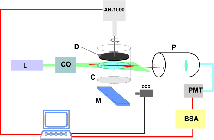
Figure 1: Overview of the swirling flow apparatus: C-fluid container, D-rotating disk, AR-1000-rheometer, CO-cylindrical optics, L-laser, M-plane mirror, CCD-digital camera, P-LDV probe, BSA-burst spectrum analyzer, PMT-photomultiplier.

The moment of inertia of the shaft of the rheometer was $I_{s}\approx 14\mu N\cdot m\cdot s^{2}$ and that of the upper plate, $I_{d}$, was about $61\mu N\cdot m\cdot s^{2}$ for setup $1$, and about $84\mu N\cdot m\cdot s^{2}$ for setup $2$. The accuracy of the angular speed measurements in constant torque mode is about $2\%$ and the accuracy of the torque measurements in the constant speed mode is about $1\%$. One has to point out here that the small rate of the fluctuations of the angular velocity is not a sufficient criterion to have a constant speed forcing. In the $\Omega$-mode, for instance, $(I_{s}+I_{d})\frac{\partial\Omega}{\partial t}$ should also be much smaller than the typical values of torque, $T$.

To obtain a detailed characterization of both the spatial structure and the temporal evolution of the flow-fields, three different experimental techniques have been alternatively used: particle image velocimetry (PIV), particle tracking velocimetry (PTV) and laser Doppler velocimetry (LDV). The cup C was machined from a single piece of optically clear perspex, to allow side and bottom view. The cup had a circular inner and a square outer horizontal cross-section (i.e. flat sides) in order to insure a distortion free illumination, and was attached to the rheometer base in such a way that view from below was possible through a mirror $\mathbf{M}$, tilted by $45^{\circ}$. As flow tracers, we have used $10\mu m$ fluorescent particles for the PIV and PTV measurements, and $1\mu m$ latex beads for the LDV measurements. For PIV and PTV the system was illuminated laterally by a thin ($30\mu$m in the center of the set-up and about $130\mu$m at the edges of the set-up) laser sheet through the transparent walls of the fluid container at the middle distance between the plates. The laser sheet was generated by passing a laser beam delivered by a $300mW$ argon-ion laser, L, through a block of two crossed cylindrical lenses, CO, mounted in a telescopic arrangement. The mirror M was used to relay images of the flow to a CCD camera (PixelFly digital camera from PCO). The camera was equipped with a regular video lens and mounted horizontally near the rheometer (Fig.1). Images were acquired with 12 bit quantization and resolution of $640\times 512$ pixels at up to $25$ frame/sec and $1280\times 1024$ at up to $12.5$ frame/sec.

The main tool for the investigation of the flow was the digital PIV technique. We acquired series of up to $2000$ pairs of flow images with the camera. A custom development of the camera control software allowed us to adjust the time delay between consecutive PIV images in relation to the local flow velocity (in order to keep the mean particle displacement in the range $5-15$ pixels). Corresponding to low values of the angular velocity of the upper disk (up to about $0.4rad/s$) the time delay was $540ms$ and then, gradually decreased down to $40ms$. The total data acquisition time was always longer than the Eulerian correlation times of the velocity (about $24$ times in the fully developed random regime). Time series of velocity fields were obtained by a multi-pass PIV algorithm taylorhypoth . The accuracy of the method was carefully checked by running test experiments with the solvent, in the same range of mean particle displacements and at similar illumination conditions. Although the instrumental error increases more or less linearly with the mean particle displacement, it never exceeded $5\%$ of the mean displacement. The spatial resolution of the PIV velocity measurements was $0.57mm$ in setup $1$ and $0.89mm$ in setup $2$. By post-processing the velocity fields, we obtained the profiles of the velocity components, fields of fluctuations of each velocity component, spatial spectra of the velocity fluctuations, velocity gradients and their fluctuations, structure functions of gradients, and Eulerian velocity correlation functions. The space-time measurements together with simultaneous global measurements of the flow resistance provided a rather complete description of the different flow regimes as a function of $Wi$ thesis ; my ; teoprl .

We also examined Lagrangian properties of the flow teo . In order to check the consistency of the PIV approach (particularly when Lagrangian trajectories were measured), flow fields have been alternatively investigated with the PTV technique. The first step of the PTV approach is the accurate particle identification in each flow image, by correlation with prototypical particle shapes, which can be either extracted from flow images, or defined manually. Then, trajectories are reconstructed by joining successive positions of the same particle on subsequent images. This has been done by a search algorithm based on an initial "guess" of the mean flow line.

Although the PIV and PTV tools are very suitable for the investigation of the spatial properties of the flow, they provide a limited time resolution and statistics. In order to overcome this limitation, the LDV technique has alternatively been used. With the LDV technique, time series of the fluid velocity are measured in a relatively small volume (typically $100\mu m\times 50\mu m\times 50\mu m$). The setup allowed measurements of one component of the velocity by LDV with two crossing and frequency shifted beams. By appropriate positioning and orientation of the beam crossing region, an azimuthal (longitudinal) velocity component, $V_{\theta}$, could be measured at different $r$ and $z$. Here $(r,\theta,z)$ are the standard cylindrical coordinates. A commercial LDV system from Dantec Dynamics Inc. was used. Two laser beams delivered by a probe (P in Fig. 1) are aligned to cross each other at an angle of $\theta=10^{\circ}$ at some point in the flow. The light scattered in the backward direction by the flow tracers present in the flow is collected by the probe P and delivered to a photomultiplier, PMT, via a fiber optic light guide. The PMT signal is processed by a real time burst spectrum analyzer, BSA. The local flow velocity is proportional to the Doppler shift of the signal. The error validated velocity data are stored on a computer via a GPIB line.

Our experiments need to be classified according to meaningful values of the non-dimensional control parameters $Re$ and $Wi$, which depend among the rest on a global shear rate. In a swirling flow between two plates, the shear rate is quite inhomogeneous over the fluid bulk, even when the flow is laminar. Therefore, the choice of a representative shear rate becomes somewhat arbitrary. We decided to consider the simple expression $\Omega R/d$ as a characteristic shear rate, and to define the Weissenberg number as $Wi=\lambda\Omega R/d$. The Reynolds number was defined as $Re=\Omega Rd\rho/\eta$.

III.2 Rheometric properties of polymer solutions

The polymer used was polyacrylamide, PAAm (from Polysciences Inc.), with a molecular weight $M_{w}=1.8\times 10^{7}Da$, as used in Ref. Nat ; NJP ; mix . Our preparation recipe was as follows: first we dissolved $0.9$ g of PAAm powder and $3$ g of NaCl into $275$ ml of deionized water by gentle shaking. NaCl was added to fix the ionic contents. Next the solution was mixed for $3$ hours in a commercial mixer with a propeller at a moderate speed. The rationale for this step is to cause a controlled mechanical degradation of the longest PAAm molecules, in order to "cut" the tail of the molecular weight distribution of the broadly dispersed PAAm sample. In a solution with a broad distribution of polymer molecular weights the heaviest molecules, which are most vulnerable to mechanical degradation, bring the major contribution to the solution elasticity, but may break in the course of the experiment. This can lead to inconsistency of the experimental results. We found empirically that the procedure of pre-degradation in the mixer leads to substantial reduction of degradation during the experiments and to substantial improvement of their consistency NJP . Finally, $9$ g of isopropanol was added to the solution (to preserve it from aging) and water was added up to $300$ g. The final concentrations of PAAm, NaCl and isopropanol in the stock solution were $3000$ ppm, $1\%$ and $3\%$, respectively. This master solution was used to prepare $80ppm$ PAAm solution in a Newtonian solvent. The Newtonian solvent was about $65\%$ saccharose in water NJP .

The rheological properties of the solvent and the polymer solution were measured with two different rheometers: the AR-1000 from TA Instruments around which the complete experimental setup was built, and a Vilastic 3 from Vilastic Scientific. The viscosity of the solvent was found to be $\eta_{s}=114mPa\cdot s$ at $22^{o}C$, and that of the solution $\eta=138mPa\cdot s$ at a shear rate of $2s^{-1}$. The polymer relaxation time $\lambda$ was measured in oscillatory tests at different shear rates, with $\dot{\gamma}$ ranging from $0.4s^{-1}$ to $3.6s^{-1}$. In the limit of $\dot{\gamma}\rightarrow 0$ the relaxation time was $\lambda(0)=4.7$ s. The solution showed a clear "shear thinning" as a function of the shear rate with the scaling $\lambda\sim\dot{\gamma}^{-\delta}$, where $\delta\simeq 0.3$, similar to what was found earlier for polymer solutions with lower molecular weight PAAm samples Ours2 .

III.3 Experimental observation of elastic instability in von Karman swirling flow

The functional dependence of the elastic instability threshold on the aspect ratio, $\epsilon\equiv d/R_{c}$, in a flow between two plates was first obtained in the experiment by Magda and Larson magda . They found an inverse dependence of the critical shear rate $\dot{\gamma}_{c}$, or of the critical Weissenberg number, $Wi_{c}=\dot{\gamma}_{c}\lambda$, on the aspect ratio, i.e.  $Wi_{c}\propto\epsilon^{-1}$. The experiment was conducted in the range of low values of $\epsilon$ between $0.024$ and $0.16$. In the later experiments similar results were obtained in the same range of $\epsilon$ by McKinley and collaborators McK ; oztekin ; McKinley . These results were found in reasonable agreement with numerical calculations. However, these numerical results presented in $Wi_{c}-\epsilon$ coordinates can be fitted by $Wi_{c}\propto\epsilon^{-0.470\pm 0.006}$ in a wide range of $\epsilon$ between $10^{-3}$ and $1$, in odds with the the above mentioned dependence $Wi_{c}\propto\epsilon^{-1}$.

We have investigated experimentally the dependence of the onset of the elastic instability on the aspect ratio of our setup. By modifying both the radius of the container, $R_{c}$, and the distance between plates, $d$, the aspect ratio $\epsilon$ was varied by about 10 times for a rather wide range of $\epsilon$, between $0.091$ and $0.882$. The onset values of the angular velocity, $\Omega_{c}$, were obtained from the dependence of the averaged torque on the angular velocity of the disk (Fig. 2). By linear approximation of this dependence on both sides of the transition point, the latter can be determined within reasonable error bars (see Fig. 2a). The Reynolds number corresponding to the onset of the elastic instability, $Re_{c}$, was of the order of unity in both setups, suggesting that the transition is of purely elastic nature. The results of these measurements together with other parameters are presented in Table 1.

${\bf{R_{c}(cm)}}$	${\bf{d(cm)}}$	${\bf{\epsilon}}$	${\bf{\Omega_{c}(rad/s)}}$	${\bf{\dot{\gamma}_{c}(s^{-1})}}$	${\bf{\lambda(\dot{\gamma})_{c}(s)}}$	${\bf{Wi_{c}}}$	${\bf{Re_{c}}}$	${\bf{\delta Wi_{c}}}$
1.7	1	0.59	0.64	1.09	4.485	4.9	1.03	1.28
1.7	1.5	0.88	0.51	0.58	5.42	3.13	1.23	1.16
2.2	1	0.45	0.82	1.8	3.85	6.95	1.72	1.19
2.2	0.5	0.23	0.85	3.74	3.1	11.6	0.89	2.45
2.2	0.2	0.091	0.88	9.68	2.33	22.54	0.37	4.94
4.7	0.5	0.106	0.45	4.23	2.98	12.62	1.0	4.6
4.7	1	0.213	0.5	2.35	3.56	8.37	2.24	1.33
4.7	1.5	0.32	0.4	1.25	4.3	5.39	2.7	1.29

Table 1: Onset values of the relevant physical quantities corresponding to the primary elastic instability

We remark that the values of the critical Weissenberg number as a function of the aspect ratio obtained from our experimental results agree fairly well with the linear stability analysis presented in oztekin ; McKinley ; McK , as shown in Fig.2b. On the other hand, the fit to the theoretical functional dependence in a wide range of $\epsilon$ between $10^{-3}$ and 1, namely $Wi_{c}\propto\epsilon^{-0.47}$, is quite different from that obtained from the experimental data: $Wi_{c}\propto\epsilon^{-0.79\pm 0.16}$. This discrepancy can be attributed to the larger aspect ratios experimentally studied by us.

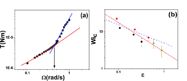
Figure 2: Dependence of the onset of the primary elastic instability on the geometric aspect ratio: (a) Torque as a function of angular velocity for the aspect ratio $\epsilon=0.88$. The full lines are linear fits. The arrow indicates the onset of the primary elastic instability. (b) Critical Weissenberg number for the onset of the elastic instability as a function of the aspect ratio. The symbols are (color online): (black) squares–$R_{c}=4.7cm$, (red) circles–$R_{c}=2.2cm$, (yellow) triangles–$R_{c}=1.7cm$. The full line is a linear fit to the data, $Wi_{c}=0.51\epsilon^{-0.79}$. The dashed line is the fit to the numerical result from oztekin , $Wi_{c}=0.62+5.42{\epsilon}^{-0.47}$.

IV Properties of elastic turbulence

IV.1 Power fluctuations and statistics of the injected power

One of the main features of the transition to elastic turbulence is the substantial growth of the flow resistance above the onset of the instability Nat ; NJP . In the case of a von Karman swirling flow, a measure of the flow resistance is either the power $P_{\Omega}$ needed to spin the upper disk at constant angular speed $\Omega$, or the power $P_{T}$ needed to spin the upper disk with constant torque $T$ applied to the shaft of the rheometer. The injected power is defined in any case as $P=T\cdot\Omega$. In our experiments, due to the smallness of $Re<16$, the inertial contribution was always low. The dependencies of the reduced average injected power, $\bar{P}/P_{lam}$ and of the rms of its fluctuations, $P^{rms}/P_{lam}^{rms}$, in a wide range of the control parameter $Wi$ in the $\Omega$ mode are presented in Fig. 3. Here $P_{lam}$ and $P_{lam}^{rms}$ are the injected power and its fluctuations before the onset of the elastic instability.

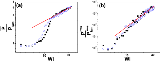
Figure 3: (a) Dependence of the scaled average power, $\overline{P}/\overline{P}_{lam}$, on the control parameter $Wi$: squares-increasing $Wi$, circles-decreasing $Wi$. The full line is a guide for the eye, with slope $Wi^{0.49}$. (b) Dependence of the scaled rms of the power fluctuations, $P^{rms}/P_{lam}^{rms}$ on $Wi$: squares-increasing $Wi$, circles-decreasing $Wi$. The full line is a power law, $Wi^{3.2}$. Data were collected in set-up $2$ in $\Omega$ forcing mode.

The data presented in Fig. 3 reveal three distinct flow regimes. For low values of the control parameter $Wi$, the reduced injected power is equal to unity. At $Wi\simeq Wi_{c}$, a primary elastic instability occurs, resulting in a sharp increase of the injected power and of the rms of its fluctuations. A further increase of the control parameter causes the flow to evolve towards a scaling regime, where both the reduced average and rms of fluctuations of the injected power scale algebraically with $Wi$ (Fig. 3): $\bar{P}/P_{lam}\propto Wi^{0.49\pm 0.05}$ and $P^{rms}/P_{lam}^{rms}\propto Wi^{3.2\pm 0.3}$.

The fluctuations of the injected power were measured for different $Wi$ in the elastic turbulence regime in two modes: $\Omega$-forcing is presented in Fig. 4 and $T$-forcing is presented in Fig. 5. For each value of $Wi$ the statistics of the power fluctuations was collected on $180000$ data points evenly sampled in time ($\Delta t\approx 38ms$). The time series of the injected power at different $Wi$ for both modes are presented in both figures. In order to avoid mechanical degradation of the the polymer solution during the long data acquisition times, separate experiments were conducted for each value of the control parameter. The local (in time) average values of the injected power did not change significantly during the total data acquisition times, suggesting that no major degradation occurred. For low values of the control parameter in the laminar regime, ($Wi<Wi_{c}$), the power fluctuations are only due to the instrumental noise. In the elastic turbulence regime, the PDFs of the power fluctuations strongly deviate from Gaussian distributions for both forcing modes. The PDFs in the $\Omega$-forcing mode have a left side skewness, while in the $T$-forcing mode -a right side skewness. Since the fluctuations of the injected power reflect fluctuations of the elastic stress averaged over the upper plate, one can conclude that the statistics of the elastic stress too must strongly deviate from Gaussian, which is a signature of intermittency. The PDFs of the reduced power fluctuations collapse on a single curve when normalized by their maximum value (see Fig. 6). Both the dependency on $Wi$ of $\bar{P}/P_{rms}$ (Fig. 3), and the skewness of the PDF in elastic turbulence suggest an analogy with similar behavior in hydrodynamic turbulence, though the reasons for the effects are entirely different pinton ; cadot .

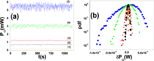
Figure 4: (a) Time series (partially shown) of the injected power in constant $\Omega$ forcing regime, for different $Wi$. The labels are: (1)-$Wi=5$, (2)-$Wi=19$, (3)-$Wi=24$, (4)-$Wi=31.5$, (5)-$Wi=40$. (b) PDF’s of the power fluctuations in$\Omega$-forcing regime for different $Wi$. The symbols are (color online): squares (orange)-$Wi=5$, left triangles (black)-$Wi=19$, up triangles (red) -$Wi=24$, diamonds (green)-$Wi=31.5$, circles (blue)-$Wi=40$. Data were collected in setup 2.

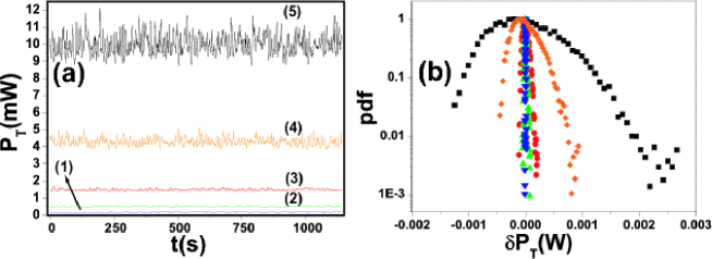
Figure 5: (a) Time series (partially shown) of the injected power in constant $T$ forcing regime for different $Wi$. The labels are: (1)-$Wi=5$, (2)-$Wi=17$, (3)-$Wi=25$, (4)-$Wi=34$, (5)-$Wi=46$. (b) PDF’s of the power fluctuations in $T$-forcing regime for different $Wi$. The symbols (color online) are: down triangles (blue)-$Wi=5$, up triangles (green)-$Wi=17$, circles (red)-$Wi=25$, diamonds (orange)-$Wi=34$, squares (black)-$Wi=46$. Data were collected in setup 2.

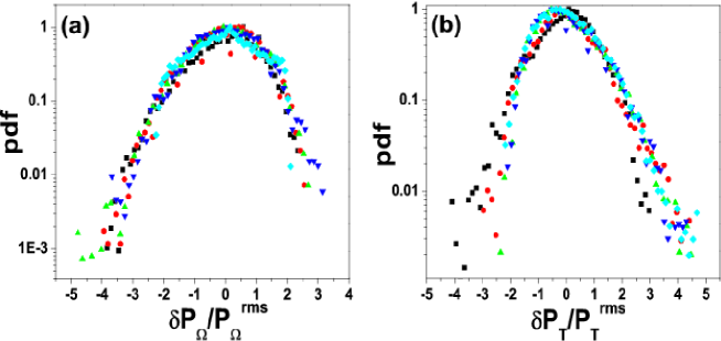
Figure 6: (a) scaled PDFs of the injected power in constant $\Omega$ forcing regime for different $Wi$. (b) scaled PDFs of the power fluctuations in constant $T$ forcing regime for different $Wi$. The symbols (color online) are: down triangles (blue)-$Wi=5$, up triangles (green)-$Wi=17$, circles (red)-$Wi=25$, diamonds (light blue)-$Wi=34$, squares (black)-$Wi=46$.

We further examined the statistics of rare and short time scale events (spikes) in the injected power series; namely we tried to quantify the characteristic width of the spikes and the characteristic time between them. To carry out this analysis, the following procedure was applied. First, all local minima and maxima were detected in each time series. Then only those minima (in the case of constant $\Omega$ forcing) and those maxima (in the case of constant $T$ forcing) that contribute to the skewness of the corresponding PDFs, are selected, i.e. those peaks which are larger than $2P^{rms}$. The values of the average time $\tau_{s}$ between two spikes, normalized by the relaxation time, are presented in Fig. 7(a), as function of $Wi$ in both $\Omega$ and $T$ modes.

We performed a similar analysis on the time series of the local azimuthal velocity measured by the LDV technique, such as those shown in the following in Fig. 17. The values of the the average time between two spikes, normalized by the relaxation time, are presented in Fig. 7(b) as function of $Wi$. We observe that the spikes in the local velocity signal occur about three time less frequently than those in the injected power series. This results in poor statistics and larger scatter, particularly for low values of $Wi$, but on the other hand is consistent with the fact that the rare events in the power time series are actually a result of space averaging (over the entire volume of the flow cell) of individual rare events in local velocity time series.

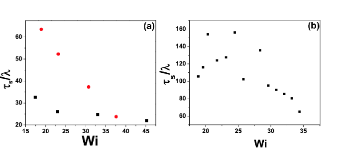
Figure 7: (a) Normalized spike periodicity, $\tau_{s}/\lambda$, in time series of the injected power vs. $Wi$: circles-constant $\Omega$ mode, squares-constant $T$ mode. (b) Normalized spike periodicity, $\tau_{s}/\lambda$, in time series of the azimuthal velocity vs. $Wi$. Data were collected at $r=2R_{c}/3$, $z=d/2$ in setup $2$.

We also computed the mean width of the spikes determined by the procedure described above. The central part of each spike was fitted by a Gaussian function, and all the fit widths $c$ for a given $Wi$ were averaged together. The results for the spikes in the series of injected power in the $\Omega$-mode are shown in Fig. 8.

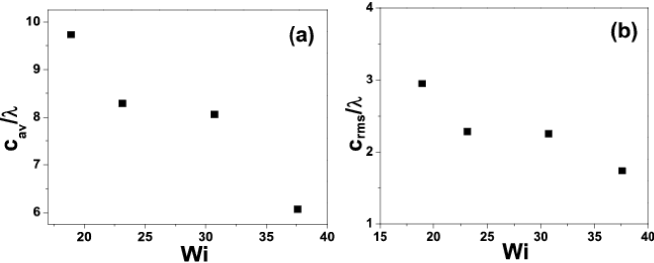
Figure 8: (a) Normalized average spike width, $c_{av}/\lambda$, vs $Wi$. (b) Normalized rms of the spike width, $c_{rms}/\lambda$, vs $Wi$. Data were collected in constant $\Omega$ mode.

IV.2 Flow structure and statistical properties of the velocity field

PIV and LDV techniques have been used in the past in various experiments and setups NJP ; taylorhypoth ; thesis ; my ; teoprl to characterize the structure of the flow field, to obtain velocity profiles and to infer and visualize the topology of the elastic von Karman flow. The visual characterization of the flow structure in a regime of elastic turbulence has been initially obtained from a few snapshots of the flow, by seeding it with light reflecting flakes ($1\%$ of Kalliroscope liquid) NJP . Already such qualitative visualization revealed the presence of a big persistent toroidal vortex, which had the dimension of the whole setup. The average flow velocity along the radial direction was measured by LDV in a few points, and the results were quite well compatible with the presence of the big vortical structure NJP .

With PIV we obtained a more complete and quantitative characterization of the global flow structure and of its dynamics. Some instantaneous vector fields of the horizontal components of the velocity, as well as the average of $2000$ instantaneous fields taken for several values of $Wi$ at a middle distance between the plates in the setup $1$ are presented in Figs. 9 and 10. The upper row of Fig. 9 shows the instantaneous vector fields at three increasing values of $Wi$, while the lower row presents averaged vector field at the same $Wi$. One can easily identify the core of the toroidal vortex that appears in all images above the threshold of the instability, and a spiral vortex that additionally occurs in the elastic turbulence regime. These flow structures and their reorganization can be also observed in separate presentations of the averaged azimuthal and radial components, and rms of fluctuations of the azimuthal velocity component of the velocity field at the same $Wi$ (see in Fig. 10,11). Below the elastic instability the profile of the average azimuthal velocity, $V_{\theta}$, exhibits a linear increase along the radius with a slope $\Omega^{-1}$ which corresponds to a rigid body rotation (see the inset in Fig. 12a), while there is no motion in the radial direction, $V_{r}\approx 0$ (Fig. 12b). Above the onset of the instability one can clearly see the creation of the core of the toroidal vortex at the cell center, and the restructuring of the radial motion thesis ; my ; teoprl .

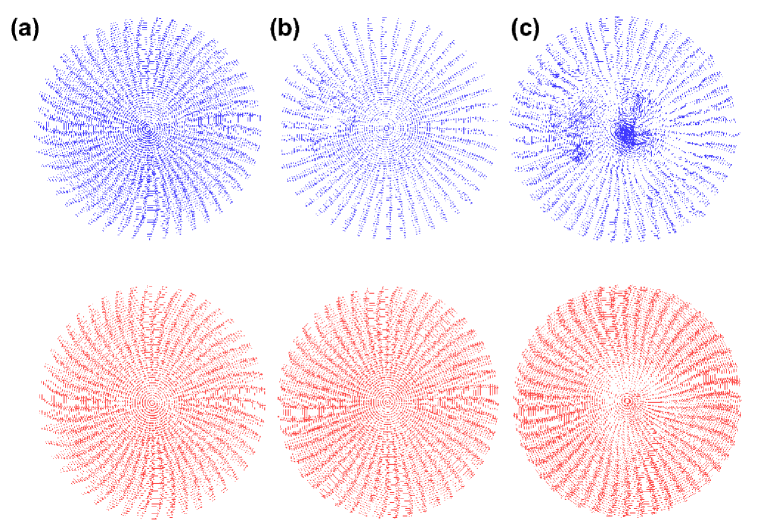
Figure 9: Instantaneous (upper row) and time averaged (lower row) velocity fields for different values of $Wi$: (a) $Wi=2.48$, (b) $Wi=9.88$, (c) $Wi=18.96$. The data were collected in setup $1$ at middle distance between plates.

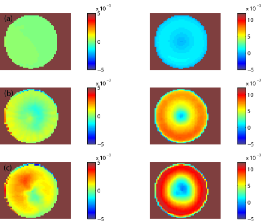
Figure 10: Distribution of the radial velocity (left column) and the azimuthal velocity components (right column) for different values of $Wi$: (a) $Wi=2.48$, (b) $Wi=9.88$, (c) $Wi=18.96$. The data were collected in setup $1$ at middle distance between plates.

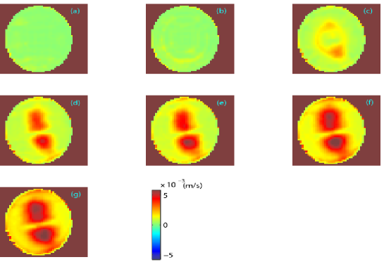
Figure 11: Fields of fluctuations of the azimuthal velocity at different $Wi$: (a) $Wi=8.32$, (b) $Wi=9.88$, (c) $Wi=11.1$, (d) $Wi=12.72$, (e) $Wi=13.83$, (f) $Wi=17$, (g) $Wi=19$. The data were collected in the setup $1$ at middle distance between plates.

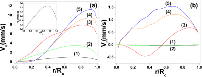
Figure 12: (a) Profiles of the average azimuthal velocity, $V_{\theta}$, for several values of $Wi$. The inset shows a typical laminar profile of the azimuthal velocity component. (b)Profiles of the average radial velocity, $V_{r}$, for several values of $Wi$. The labels are: (1)-$Wi=2.48$, (2)-$Wi=4.41$, (3)-$Wi=11.1$, (4)-$Wi=15$, (5)-$Wi=18$. Data were collected in set-up $1$ at middle distance between plates.

Large toroidal vortexes driven by the hoop stress are actually quite well known to appear in swirling flows of elastic fluids bird ; Boger2 . The inhomogeneity of the shear rate profile in the primary laminar flow has long been recognized as their common origin. In our system this vortex first arises as a stationary structure at low shear rates, and leads to some increase in flow resistance even before the elastic instability NJP . Therefore, one concludes that the transition to elastic turbulence in the swirling flow between two plates is mediated by this vortex. The toroidal vortex is providing a smooth, large scale velocity field (see lower panels in Fig. 9), which is randomly fluctuating in time (upper panels in Fig. 9), and in which the fluid and the embedded stress tensor are chaotically advected. This type of advection can create variations of stress in a range of smaller scales, which may cause small scale fluid motion Volodya ; Volodya2 . This is analogous to the generation of small scale variations of scalar concentration in chaotic mixing by large fluctuating vortexes.

Above the instability threshold, the large scale toroidal vortex is also responsible for the ring-shaped topology of the fluctuation field of the azimuthal velocity, $V_{\theta}^{rms}\equiv\overline{V_{\theta}^{2}}^{1/2}$ (Fig. 11). The velocity fluctuations in the laminar regime are only due to instrumental noise (panel (a) in Fig. 11). The average radial velocity changes its sign at about a half of the radius (see Fig. 12b). At higher values of $Wi$, the toroidal vortex forces the transition to elastic turbulence. This is accompanied by a second reorganization of the flow structure, with the appearance of a fluctuating spiral vortex (Figs. 9,10) and takes part in the scaling regime of $P$, $P_{rms}$ (see Fig. 3). Movie animations of the velocity fields evidence that this secondary fluctuating vortex is carried around and “rides” on top of the primary vortical flow. At the same time the circular symmetry of $V_{\theta}^{rms}$ is broken into a dipolar one (see Fig. 11). The radial profiles of $V_{\theta}$ and $V_{r}$ also change drastically. The structural transitions in the flow are also reflected in the average radial gradients of the azimuthal velocity and in the average vorticity field, as presented in Fig. 13 for various values of $Wi$.

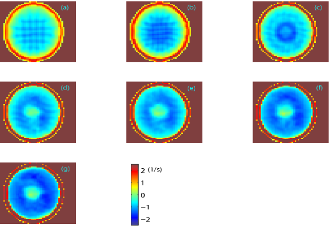
Figure 13: Average vertical component of the vorticity, $\omega_{z}$, at different $Wi$: (a) $Wi=8.32$, (b) $Wi=9.88$, (c) $Wi=11.1$, (d) $Wi=12.72$, (e) $Wi=13.83$, (f) $Wi=17$, (g) $Wi=19$. Data were collected in setup $1$ at middle distance between plates. The gridded pattern visible in panels (a), (b) is an artifact of combined peak locking and numerical differentiation effects and should be disregarded.

Another way to characterize a turbulent flow is to display the radial profiles (averaged over the azimuthal coordinate) of the turbulent intensity, defined as $I_{t}=\frac{V_{\theta}^{rms}}{V_{\theta}}$ at several values of $Wi$ (see Fig. 14) teoprl . The velocity fluctuations in the laminar regime occur only due to instrumental errors. Above the elastic transition $I_{t}$ increases sharply but remains rather uniform on the level between $20$ and $30\%$ in a peripheral region for the radius ratios, $r/R_{C}$, between $0.2$ and $1$. In the regime of elastic turbulence $I_{t}$ further increases, and its dependence on $Wi$, presented in the inset in Fig. 14, exhibits the power-law scaling, $I_{t}\sim Wi^{0.49\pm 0.06}$ thesis ; my .

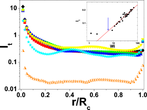
Figure 14: Turbulence intensity versus the reduced radial coordinate at different $Wi$: diamonds-$Wi=31.56$, squares- $Wi=27.73$, circles-$Wi=23.67$, up triangles-$Wi=19.29$, down triangles-$Wi=15.48$, stars-$Wi=7.54$, half filled triangles-$Wi=2.82$. The inset shows the dependence of the turbulence intensity on $Wi$ at $r/R_{c}=0.85$ obtained from LDV measurements. The full line is a power law fit, $I_{t}\propto Wi^{0.49\pm 0.06}$. The arrow indicates the onset of the elastic instability. The data were collected in setup 2.

The PIV measurement of time dependent velocity fields allowed us to calculate the average velocity gradients and vertical vorticity, and rms of their respective fluctuations, without involving the Taylor hypothesis that can be questionable for a smooth random flow taylorhypoth ; thesis . The typical radial distribution of the velocity gradients and of vorticity, averaged spatially over the azimuthal coordinate and temporally over $2000$ images is rather uniform in the bulk for all $Wi$, but increases sharply near the wall (see Fig. 15(a)), while the rms of the velocity gradients and vorticity gradually increases with the radius (Fig. 16(a)). The dependence of the average vertical vorticity on $Wi$ is displayed in Fig. 15(b). At higher values of $Wi$ one finds a gradual growth of the vorticity both in the bulk and near the wall. On the other hand, the plot in Fig. 16(b) shows the $Wi$ dependence of the rms of the vorticity, $\omega_{rms}$, scaled by $\lambda$, at several locations along a radius in the bulk. The scaled rms of the vorticity saturates in the elastic turbulence regime at a $Wi$ between $12$ and $35$, that is consistent with the recent theoretical prediction. Similar behavior is shown by all the components of the velocity gradient, and is consistent with the theoretical predictions, though the saturation value $\omega_{z}^{rms}\cdot\lambda\approx 2$ is higher than expected Volodya ; Volodya2 . The latter means probably that the nonlinearity of the polymer elasticity also contributes to the saturation of the elastic stress lebedev ; chertkov (see further discussion of this issue).

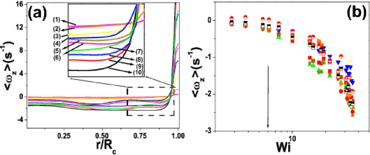
Figure 15: (a) Profiles of the vorticity $\langle\omega_{z}\rangle$ averaged spatially in the azimuthal direction and temporally over $2000$ images, for different $Wi$. The labels are: (1)-$Wi=2.82$, (2)-$Wi=5.4$, (3)-$Wi=10$, (4)-$Wi=14.48$, (5)-$Wi=17.43$, (6)-$Wi=19.29$, (7)-$Wi=26.13$, (8)-$Wi=27.73$, (9)-$Wi=32.3$, (10)-$Wi=34.5$. (b) Dependence of the average vorticity on $Wi$ at different radial positions $r/R_{c}$,: left triangles-$0.1$, down triangles-$0.2$, squares-$0.33$, up triangles-$0.4$, stars-$0.5$, circles-$0.66$, right triangles-$0.7$, half filled squares-$0.8$, half filled circles-$0.9$. The arrow marks the onset of the elastic instability. The data were collected in setup $2$.

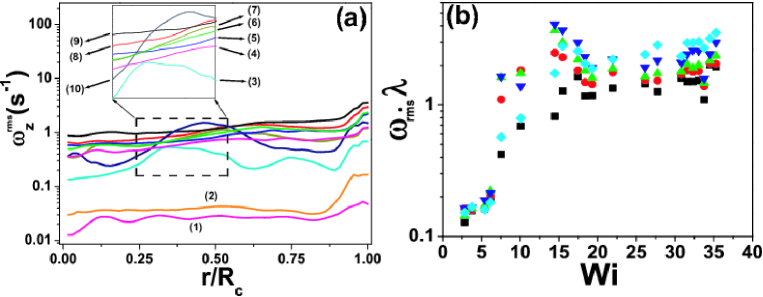
Figure 16: (a) Profiles of the rms of the fluctuations of the vorticity, $\omega_{z}^{rms}$, at different $Wi$. The labels are: (1)-$Wi=2.82$, (2)-$Wi=5.4$, (3)-$Wi=10$, (4)-$Wi=14.8$, (5)-$Wi=17.43$, (6)-$Wi=19.29$, (7)-$Wi=26.3$, (8)-$Wi=26.3$, (9)-$Wi=27.73$, (10)-$Wi=32.3$, (b) Dependence of the scaled rms of the vorticity, $\omega_{rms}\cdot\lambda$, on $Wi$ at different radial positions $r/R_{c}$: full squares, $0.2$; open squares, $0.33$; full circles, $0.4$; open circles, $0.5$; diamonds, $0.66$. The data were collected in setup $2$.

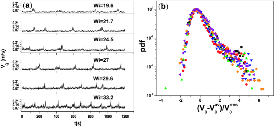
Figure 17: (a) Time series of azimuthal velocities, $V_{\theta}$, for several values of $Wi$. (b) PDFs of normalized azimuthal velocities for various $Wi$: squares-$19.6$, circles-$21.7$, up triangles-$24.5$, down triangles-$27$, diamonds-$29.6$, left triangles-$33.2$. Data were collected in setup $2$, at $z=d/2$ and $r=2R_{c}/3$.

Time series of azimuthal velocity obtained from LDV measurements for several values of $Wi$ are displayed in Fig. 17(a). As $Wi$ increases, the velocity signal becomes increasingly intermittent. PDFs of the normalized azimuthal velocity, $(V_{\theta}-V_{\theta}^{av})/V_{\theta}^{rms}$, are shown in Fig. 17(b). The right side skewness of the PDFs is due to the rare events (spikes) which intermittently occur in the velocity signal (Fig. 17(a)), which are probably related to the dynamics of the randomly fluctuating spiral vortex previously discussed.

In order to understand better the structure of the flow in the regime of elastic turbulence, we have studied the dependence of the statistics of the azimuthal velocity on the radial coordinate, for a fixed value of $Wi=36.1$ and a given vertical coordinate, $z=d/2$. As illustrated in Fig. 18(a), in the central ($r=0$) and peripheral ($r=15R_{c}/16$) flow regions, the velocity signal shows no significant intermittency, whereas around $r=R_{c}/2$ it is strongly intermittent. The radial dependence of the level of intermittency reflects the presence of the randomly fluctuating spiral vortex (where, probably, $r=R_{c}/2$ corresponds to the arm of the spiral). This behavior is also reflected in the PDFs of the normalized azimuthal velocity presented in Fig. 18(b): near the center and the vertical wall of the cell, the distributions are symmetric and single peaked whereas around $r=R_{c}/2$ they become strongly skewed and doubly peaked.

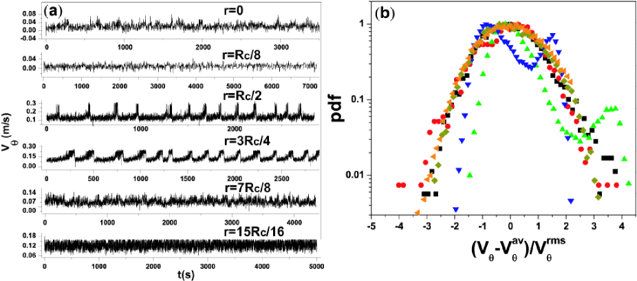
Figure 18: (a) Time series of azimuthal velocities, $V_{\theta}$, for $Wi=36.1$ at several radial positions, $r$. (b) PDFs of the normalized azimuthal velocity, for $Wi=36.1$, at several radial positions $r$: squares-$0$,circles-$R_{c}/8$,up triangles-$R_{c}/2$,down triangles-$3R_{c}/4$,diamonds-$7R_{c}/8$, left triangles-$15R_{c}/16$. The data were collected in setup $2$, at $z=d/2$.

Fig. 19 shows PDFs of the normalized accelerations as calculated from the temporal LDV measurements, $(Y(t)-Y_{av})/Y_{rms}$, where $Y(t)\equiv\frac{dV(t)}{dt}V_{av}^{-1}$. We note that all the data for several values of $Wi$ collapse on a single curve remarkably well, and that moreover the PDFs show clear exponential tails.

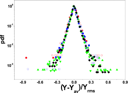
Figure 19: PDFs of normalized accelerations for various $Wi$: full circles-$14$; open circles-$16.2$; full squares-$19.8$; open squares-$22.3$; up-triangles-$26.3$; down-triangles-$30.7$; diamonds-$38.9$. The data were collected in setup $2$ at $z=d/2$ and $r=2R_{c}/3$.

The PIV data allow us also to calculate various correlation and structure functions of velocity, velocity gradients, and vorticity. Their scalings can give information on the degree of deviation from a Gaussian random field, a standard way in hydrodynamics to quantify intermittency and to compare it with the corresponding scaling in known cases.

The spatial power spectra of the velocity were obtained from PIV data by averaging $2000$ instantaneous spatial spectra. Although the finite spatial resolution of PIV, which limits the accessible range of wave numbers, leads to an artificial cut-off at $k\sim 3000m^{-1}$, a power law decay $k^{-\delta}$ with $\delta\simeq 3.5$ is clearly observed (Fig. 20) thesis ; my . This decay is consistent with the scaling obtained earlier for the velocity power spectra in the frequency domain Nat ; NJP ; my . The large value of the exponent $\delta$ implies that the power of fluctuations decays very quickly as the size of eddies decreases. The main contribution to the fluctuations of both the velocity and the velocity gradients is therefore due to the largest eddies, and the power of the latter should scale as $k^{-(\delta-2)}$.

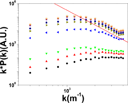
Figure 20: Power spectra of the fluctuations of the azimuthal velocity component at different $Wi$: circles-$Wi=4.41$, up triangles-$Wi=5.72$, down triangles-$Wi=8.32$, left triangles $Wi=11.1$, right triangles-$Wi=12.7$, hexagons-$Wi=13.8$, diamonds-$Wi=16$, half filled squares-$Wi=18$, empty circles-$Wi=19$. The solid line is the power law $k^{-3.5}$. The data were collected in setup $1$.

The agreement between the velocity spectra measured at a single point in frequency domain Nat ; NJP and the spectra measured directly in $k$-domain thesis ; my deserves a brief discussion. Following Lumley lumley , the relation between the spatial spectrum $P(k)$ and the frequency spectrum $P(f)$ can be written as

$$P(k)=V\cdot P(f)-\frac{I_{t}^{2}}{2}\cdot\frac{d^{2}\left(k^{2}P(k)\right)}{dk^{2}}+O\left(I_{t}^{4}\right),$$ (8)

where $I_{t}=V_{\theta}^{rms}/V_{\theta}$, $V_{\theta}^{rms}\equiv{\overline{V_{\theta}^{2}}}_{t}^{1/2}$ and $V_{\theta}$ are the rms of fluctuations of the azimuthal velocity and the average azimuthal velocity, respectively. If $P(k)\propto k^{\delta_{2}}$ and $P(f)\propto f^{\delta_{1}}$, the equation above leads to:

$${\delta_{2}-\delta_{1}}\propto\frac{\log\left[1+\frac{I_{t}^{2}}{2}\cdot\delta_{2}\cdot(\delta_{2}+2)\right]}{\log(k)}\,.$$ (9)

If one plugs into the last equation $\delta_{2}\approx-3.5$, the difference between the exponents is (for $k\approx 1000m^{-1}$) as small as ${\delta_{2}-\delta_{1}}\approx 0.1$. Thus, the experimental resolution does not allow us to observe the difference in the scaling exponents for the spatial and temporal spectra thesis .

Next, let us focus on the typical spatial and temporal correlation scales in elastic turbulence. A typical scale, at which elastic stress is correlated can be estimated as $L=2\pi\int P(k)dk/\int k\,P(k)dk$. In our setup and in the elastic turbulence regime, one gets $L\simeq 5.9$ cm, i.e. on the order of the cell size. The Eulerian correlation time is defined as $\tau_{c}=\int t\,C(t)dt/\int C(t)dt$, where $C(t)=\overline{V(T)V(T+t)}/\left(V^{rms}\right)^{2}$ is the Eulerian correlation function. Figure 21 presents the normalized $\tau_{c}/\lambda$ as a function of $Wi$ at some radial positions in the cell. The correlation time drops significantly in the transition region and then saturates in the elastic turbulence regime, as the rms of the vorticity (and velocity gradients) fluctuations do. The related saturation of both the Lyapunov exponents of the Lagrangian trajectories, already reported teo , and the reduced velocity correlation time, $\tau_{c}/\lambda$, shown in Fig. 21 (in the same range of $Wi$) just reinforces the observation. We point out that the inverse saturated value of correlation time is of the order of the saturated value of $\omega_{z}^{rms}$ and $\lambda^{-1}$, as predicted by theory Volodya ; Volodya2 .

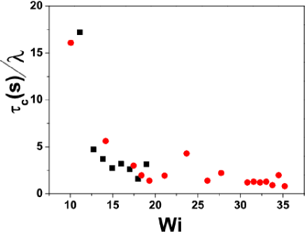
Figure 21: Scaled Eulerian correlation times of the azimuthal velocity component as function of $Wi$: squares-setup $1$, circles-setup $2$.

Using the PIV data one can also calculate the structure functions of the velocity gradients, defined as

$$S_{p}(r)=\left\langle\left|\frac{\partial V_{\theta}(r_{0}+r)}{\partial r}-\frac{\partial V_{\theta}(r_{0})}{\partial r}\right|^{p}\right\rangle_{r_{0}}$$ (10)

and shown in Fig. 22. As for inertial turbulence, we can look for a scaling in the spatial range corresponding to the power law decay of the velocity spectra (Fig. 20) in the form: $S_{p}(r)=r^{\zeta_{p}}$. The dependence of the normalized scaling exponent, $\zeta_{p}/\zeta_{4}$, on the order of the structure functions, $p$, is presented in the inset of Fig. 22 for all flow parameters mentioned above. For comparison, the structure functions of the vorticity, of the injected power at constant $\Omega$, $P_{\Omega}$, and constant torque, $P_{T}$, were also calculated, and the results of the analysis for the normalized scaling exponent were also plotted in the inset of Fig. 22. All these dependencies are rather close to that obtained for a passive scalar in elastic turbulence, presented on the same plot and based on our published data Teo ; thesis ; all of them deviate from a linear dependence that is characteristic of a Gaussian distribution Shr .

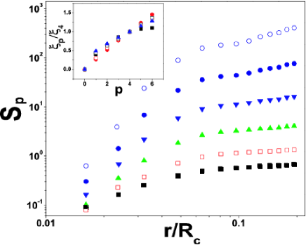
Figure 22: Structure functions of the velocity gradients of order $p$ up to $6$ as a function of the scaled radius. Inset: normalized scaling exponent vs. $p$ for: injected power $P_{\Omega}$- full circles; injected power $P_{T}$- open circles; passive scalar- full squares; vorticity- open squares; velocity gradient- up-triangles.

It is worth to make here some remarks about the applicability of the Taylor hypothesis to flows which are spatially smooth random in time, such as is elastic turbulence, which we have studied experimentally in more detail in taylorhypoth . On one hand, the comparison of the power spectra of the velocity in frequency and wave number domain suggests that the Taylor hypothesis is applicable at least in regions close to the wall. On the other hand, from Fig. 14 one can learn that in the central flow region, at $r/R_{c}<0.2$, the rms of the velocity fluctuations becomes much larger that the mean velocity, fact which is normally thought to violate the assumptions of the hypothesis. By detailed analysis of cross-correlations as well as of the structure functions of the velocity fluctuations, it was indeed shown in taylorhypoth that strong velocity fluctuations near the cell center prevent, and flow smoothness and lack of scale separations close to the boundaries limit the quantitative applicability of the Taylor hypothesis. However, this deficiency can be corrected by a proper choice of the advection velocity, so that a corrected Taylor hypothesis is applicable to most parts of this chaotic flow.

IV.3 Velocity and velocity gradient profiles and the boundary layer problem

To learn more about the flow field generated by elastic turbulence, we investigated in detail the structure of horizontal and vertical velocity boundary layers for different values of $Wi$ and fluid viscosity. The vertical profile of the azimuthal velocity, $V_{\theta}$, in the laminar flow of the pure solvent is nearly a straight line NJP ; my . The transition to elastic turbulence flow significantly changes the distribution of $V_{\theta}^{av}$, producing a high shear layer near the upper plate and a low shear region near the middle of the gap (at $z/d=0.5$). Such a distribution of $V_{\theta}^{av}$ is reminiscent of average velocity profiles in usual high $Re$ turbulence. In Fig. 23 we present the average azimuthal velocity profiles measured by LDV in a vertical plane at $r=3R_{c}/4$ of the setup $2$ with $d=2$cm height in $65\%$ of saccharose solution and normalized by the velocity value at the disk, $\tilde{V}_{\theta}(z/d)=V_{\theta}^{av}(z/d)/V_{\theta}^{up}$. In Fig. 24 the same data for different $\Omega$ are collapsed on a single curve, after subtraction the $z$-dependence of the average velocity in the bulk for each curve, that is $\tilde{V}_{\theta}^{*}(z/d)=\tilde{V}_{\theta}(z/d)-\tilde{V}_{\theta}(1/2)-\frac{z}{d}\left.\frac{\partial\tilde{V}_{\theta}(z/d)}{\partial\left(z/d\right)}\right|_{1/2}$, where $\frac{\partial\tilde{V}_{\theta}(z/d)}{\partial\left(z/d\right)}$ is obtained from a linear fit of the data points. Similar velocity profiles were also obtained with polymer solutions with saccharose content reduced to 60% and 50%. We defined the boundary layer width $w$ as the intersection abscissa of the linear fits for the bulk and near-the-wall parts of the velocity profile. It is clear from the plot that $w$ is independent of $\Omega$ for each solution and is seen to depend only on the solution viscosity, whereas we obtained the fit $w\propto\eta^{0.26\pm 0.05}$ (upper inset of Fig. 24). Fluctuations of the azimuthal velocity are small near the upper plate, reach a maximum at $z/d\simeq 0.1$, and start to decrease at larger $z$. Again, such distribution of $V_{\theta}^{rms}$ along $z$ is reminiscent of the velocity fluctuations in the boundary layer of turbulent flows of a Newtonian fluid landau ; Tritt . An example of the profile of the rms of the azimuthal velocity $V_{\theta}^{rms}$, obtained at various $\Omega$ in the setup $2$ with height $d=1$cm, is shown in Fig. 25. Well-defined peaks appear at the same position, which does not depend on $\Omega$, and match the boundary layer thickness $w$ found with the previous analysis of the average velocity profiles, and displayed in Fig. 24.

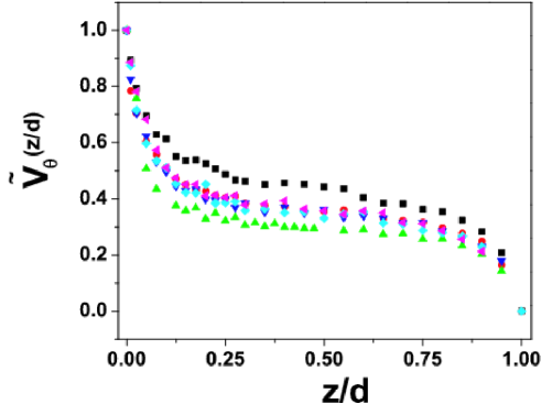
Figure 23: Vertical profile of the average azimuthal velocity, normalized by its maximum value at the disk, measured by LDV in setup $2$, with $d=2$cm, in a vertical plane at $r=3R_{c}/4$, in a 65% saccharose polymer solution, for several values of $\Omega$: full squares (black)-$5s^{-1}$, circles (red)-$4s^{-1}$, up-triangles (green)-$3s^{-1}$, down-triangles (blue)-$2.5s^{-1}$, diamonds (cyan)-$2s^{-1}$, left-triangles (magenta)-$1.5s^{-1}$.

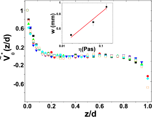
Figure 24: Compensated vertical profile of the average azimuthal velocity $\tilde{V_{\theta}^{*}}$(see text), for several values of $\Omega$: full squares-$5s^{-1}$; circles-$4s^{-1}$; up-triangles-$3s^{-1}$; down-triangles-$2.5s^{-1}$; diamonds-$2s^{-1}$; open squares-$1.5s^{-1}$. Inset: boundary layer thickness $w$ vs. solution viscosity; the solid line is the fit $w\propto\eta^{0.26\pm 0.05}$. Data measured in the same setup as data of Fig. 23.

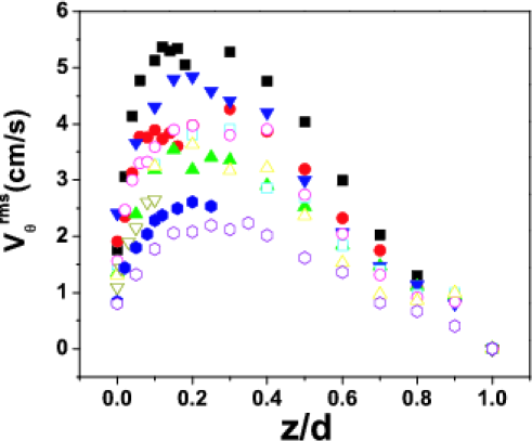
Figure 25: Profile of the rms of the azimuthal velocity measured by LDV in a vertical plane at $r=3R_{c}/4$, in setup $2$ with $d=1$cm height, in 65% of saccharose solution, for several values of $\Omega$: full squares-$6rad/s$, full circles-$5.5rad/s$, full up triangles- $5rad/s$, full down triangles-$5.5rad/s$, empty squares-$4rad/s$, empty circles-$3.7rad/s$, empty up triangles-$3.5rad/s$, empty down triangles- $3rad/s$, full hexagons-$2.5rad/s$, empty hexagons-$2rad/s$.

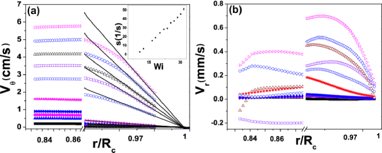
Figure 26: Near-wall profiles of the velocity in a horizontal plane at $z=d/2$, for various values of $Wi$ in setup 2, with $65\%$ saccharose polymer solution. (a) Radial profiles of the tangential velocity component $V_{\theta}$. The full lines are linear fit functions. The inset shows the dependence of the slope of the linear fit functions, $s$, on $Wi$. (b) Radial profiles of the radial velocity component $V_{r}$. The symbols are: full squares-$Wi=2.4$, full up triangles-$Wi=4$, full diamonds-$Wi=5.9$, full right triangles-$Wi=7$, full stars-$Wi=10.6$, empty circles-$Wi=16.6$, empty squares-$Wi=20.3$, empty up triangles-$Wi=23.8$, empty diamonds-$Wi=23.8$, empty right triangles-$Wi=30.2$.

We also measured by PIV radial profiles of both the azimuthal and the radial velocity in a horizontal plane at $z=d/2$ in the vicinity of the vertical wall of the cell, shown in Fig. 26(a,b). As shown in Fig. 26a, the azimuthal velocity component $V_{\theta}$ can be fitted by a linear function in the vicinity of the wall. This agrees with the requirements of incompressibility, boundary condition for the velocity and smoothness of the velocity field, as pointed out in Ref. Turitsyn .

In the regime of elastic turbulence the slopes of the linear fit functions increase monotonically with $Wi$ (see the inset in Fig. 26a). Using the fits one can determine the width of the vertical (close to the exterior cylindrical wall) boundary layer, $w_{\theta}$, of the azimuthal velocity.

As shown in Fig. 27, the width of the vertical boundary layer, $w_{\theta}$, decreases abruptly above the onset of elastic instability and saturates in the regime of elastic turbulence, for large values of $Wi$. Unfortunately the limited accuracy of measurements of the radial velocity component near the wall (note that radial velocities are about two orders of magnitude smaller than the azimuthal ones) did not allow us to assess beyond doubt the functional behavior of the radial profiles of radial velocity component near wall, presented in Fig. 26b.

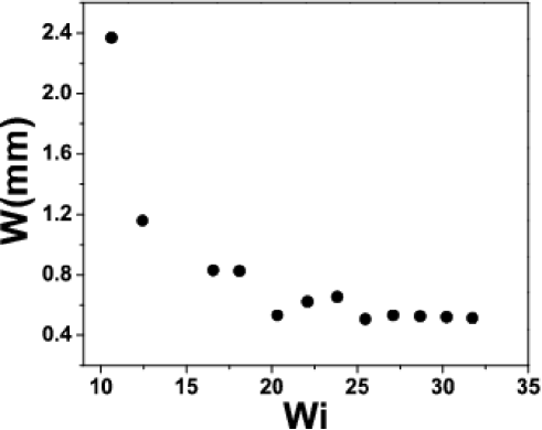
Figure 27: Dependence of the width of the vertical boundary layer, $w_{\theta}$ (defined via the width of the linear part of the near wall $PIV$ profiles of the tangential velocity component) on $Wi$. Data were collected in setup $2$.

In order to improve the spatial resolution of the velocity field measurements near the wall, and particularly to resolve the horizontal boundary layer by looking at the rms of the radial gradient of the azimuthal velocity, $(\partial V_{\theta}/\partial r)^{rms}$, the field of view of the PIV measurements was reduced down to $10mm$ in the radial direction. The radial profiles of $(\partial V_{\theta}/\partial r)_{norm}^{rms}$ near the wall for various values of $Wi$ in the elastic turbulence regime are shown in Fig. 28. As in the case of the average velocity in the vertical plane (Fig. 24), the bulk part of the radial dependence fitted by a line was subtracted for each curve. Well-defined peaks, positioned independently of $Wi$, can easily identified inside the velocity boundary layer. We would like to point out that the value of $(\partial V_{\theta}/\partial r)^{rms}$ at the maximum exceeds up to two orders of magnitude its bulk value (see Fig. 16(b)).

The same data were also used to determine the average value of $(\partial V_{\theta}/\partial r)^{rms}$ in the boundary layer. The latter was obtained from widths of distributions of the slopes of the radial dependence of the azimuthal velocity in the boundary layer region, for each value of $Wi$. These average values of $(\partial V_{\theta}/\partial r)^{rms}$ scaled by $\lambda$, in the vertical boundary layer of the setup $2$ with cell height $d=1$cm are shown in Fig. 29 as function of $Wi$. A clear increase of $(\frac{\partial V_{\theta}}{\partial r})^{rms}\cdot\lambda\gg 1$ in the boundary layer, in contrast to its saturation value in the bulk, $(\frac{\partial V_{\theta}}{\partial r})^{rms}\cdot\lambda\approx 2$, was found in the same range of $Wi$ (see further discussion).

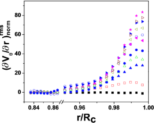
Figure 28: Normalized radial profiles of rms of the azimuthal velocity gradients, $({\partial V_{\theta}/\partial r})_{norm}^{rms}$ in the vicinity of the vertical wall, for various values of $Wi$ (color online): full squares-$Wi=10.6$, empty squares-$Wi=12.4$, full up triangles-$Wi=16.5$, empty up triangles-$Wi=18.1$, full circles-$Wi=20.3$, full left triangles-$Wi=22$, empty circles-$Wi=23.8$, empty left triangles-$Wi=25.4$, full right triangles-$Wi=27$, empty right triangles-$Wi=28.6$, stars-$Wi=30.2$. Data were collected using PIV in setup $2$ with a $65\%$ saccharose polymer solution, in a horizontal plane at $z=d/2$.

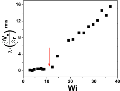
Figure 29: Scaled rms of the velocity gradients in the boundary layer vs $Wi$. The arrow indicates the onset of the primary elastic instability.

IV.4 Discussion: role of the elastic stresses in elastic turbulence in a finite size cell.

Let us summarize our different experimental observations, discuss some of their implications, and delineate a comprehensive picture of the phenomenon called elastic turbulence.

(i) The rms of the vorticity (and that of velocity gradients) saturates in the bulk of the elastic turbulent flow, leading to the saturation of the elastic stress. The saturation of $\omega_{rms}$ at high values of $Wi$ in the elastic turbulence regime, observed in the data in Fig. 16, gives us the possibility to test which of the two theoretical mechanisms is responsible for it: either the feedback reaction of polymer molecules on the flow lebedev or the nonlinearity of polymer elasticity chertkov . The local Weissenberg number can be estimated from Fig. 16 as $Wi^{\prime}=\omega_{rms}\cdot\lambda\simeq 2$, which exceeds the unit value predicted by the model with feedback of linear molecule elasticity, discussed by Volodya ; Volodya2 . We conclude that the nonlinearity of the polymer elasticity may also contribute to the saturation of the elastic stresses chertkov . The saturation of the elastic stress in the bulk also naturally explains the power-law behavior of the average injected power, $\frac{\bar{P}}{\bar{P}_{lam}}\sim Wi^{0.49}$, seen in the plot in Fig. 3. Indeed, the injected power is proportional to the torque, $P=T\cdot\Omega$. The latter is just the shear stress averaged over the upper plate, and its growth above the instability threshold occurs solely due to the elastic stress, $\bm{\tau}_{p}$, stretch . In the elastic turbulence regime, however, the theory predicts $\tau_{p}\sim\eta/\lambda$. On the other hand, it was found that, due to shear thinning of the solution used, $\lambda\sim\Omega^{-0.3}$. Thus, the theoretically expected growth of the mean injected power with respect to its laminar value, $\bar{P}_{lam}$, should be solely due to the elastic stress and have the following power-law scaling: $\frac{\bar{P}}{\bar{P}_{lam}}\sim\tau_{p}\sim Wi^{0.43}$ which is rather close to the scaling we observed experimentally.

Next, we made three main observations (ii)-(iv) below, which extend further the formal similarity with hydrodynamic turbulence, despite the distinctively different underlying mechanism for intermittency. Our findings in the statistics and structure of the velocity field have to be related to the finite size of the experimental vessel, whereas the current theory describes elastic turbulence in an unbounded domain Volodya ; Volodya2 . One can expect to find new effects in statistical and scaling behavior, similar to those recently studied both theoretically and experimentally for a passive scalar advected by a smooth random flows in bounded geometries chertkov2 , such as that in a channel considered by Teo .

As was already pointed out in the Introduction, there is a deep analogy in the statistical behavior of elastic turbulence, of the fast magneto-dynamo, and for the passive scalar dispersion in the Batchelor regime. As was shown in Section II.4, the elastically driven random flow can be considered as turbulence of the elastic stress field; all its statistical properties can be explained by the interplay of (a) stretching and folding of fluid elements carrying elastic stresses on Lagrangian trajectories in the Batchelor regime, (b) dynamo effect leading to the saturation of stresses in the bulk flow, and (c) homogeneous linear damping of the stress. Thus, since the dynamics of the elastic stress tensor can be reduced to the dynamics of the vector field $\mathbf{B}$, this scenario is very close to that found in the fast magneto-dynamo except that (c) is replaced by the diffusive dissipation of the magnetic field. On the other hand, the passive scalar problem differs from elastic turbulence (besides the fact that in this case a vector is replaced by a scalar) in the item (b), since in the former the feedback reaction on the flow is absent. However, in spite of the fact that there is no exact similarity between these three problems, the main ingredient (a) gives a basis for the similarity in statistical and scaling behavior of these systems. Taking into account the similarity, we can extend it to statistical properties of elastic turbulence in a finite size vessel.

(ii) The rms of the velocity gradients $\left(\frac{\partial V_{\theta}}{\partial r}\right)^{rms}$ or $\omega^{rms}$, and thus the elastic stress, grows linearly with $Wi$ in the boundary layer (see Fig. 29), near the driving disk. The rms of the velocity gradients saturates in the bulk (see Fig. 16). Moreover, the values in the boundary layer are one to two orders of magnitude larger than in the bulk. All this implies that a boundary layer is formed, with an excess of the elastic stress is concentrated in it.

(iii) The PDFs of the injected power $\delta P_{\Omega}/P_{\Omega}^{rms}$, at either constant angular speed or torque, show skewness and exponential tails, which both indicate intermittent statistical behavior. Also the PDFs of the normalized accelerations, which can be related to the statistics of velocity gradients via the Taylor hypothesis, exhibit well pronounced exponential tails. We can match this facts and the emergence of the boundary layer with the following scenario: the forcing from the moving boundary (the upper disk) produces an accumulation of the elastic stress in the boundary layer due to a constant flux of momentum from the upper boundary. Elastic stress is intermittently injected into the bulk by random release events. Whenever that happens, the power on the disk decreases. Constant build-up and sudden release would thus explain the skewness of the PDF toward small values of the injected power, while intermittency would be the origin of the observed exponential tails. The exponential tails in the PDF of the velocity gradients and accelerations (Fig. 17-19) can be also explained in the same way, except that for them the symmetry of the PDF is preserved due to injections from both the upper and lower boundary layers.

However, the most surprising and striking feature of elastic turbulence observed is (iv), the presence of a velocity boundary layer and the emergence of a new length scale. Since elastic turbulence is a turbulence of an elastic stress field, one can expect primarily the appearance of a boundary layer in the elastic stress field. We observe in addition the presence of a velocity boundary layer, which just reflects some of the features of the boundary layer of the elastic stresses (rms of the velocity gradients). The measured thickness of the velocity boundary layer is much smaller than the vessel size. To argument further on it, we note that the picture presented in point (iii) is in close analogy with the turbulent advection of a passive scalar in the Batchelor regime in a finite channel flow, where the excess of tracer from the boundary layer is intermittently injected into the bulk chertkov2 ; Teo . There the boundary layer for a passive scalar (mixing boundary layer) results from zero boundary conditions for the flow velocity components along and towards the wall. This leads to less effective advection of the passive scalar near the wall, causing an accumulation in the near-wall region, and thus a boundary layer in which the statistics of the scalar is different than that in the bulk flow. In the case of the passive scalar, the mixing boundary layer and the new length scale appear due to the existence of a small parameter, the inverse Peclet number, $Pe^{-1}=(D/V^{rms}L)\ll 1$, where $D$ is the diffusion constant, and $L$ is the vessel size. Then, as predicted theoretically chertkov2 and confirmed experimentally Teo , the mixing boundary layer width is found to scale as $w\propto Pe^{-1/4}\propto D^{1/4}$. Intermittent ejection of the tracer into the bulk, analogous to the intermittent injection of elastic stresses in elastic turbulence, reduces the effectiveness of mixing, increases the mixing length, and causes stronger (power-law) dependence of the mixing length on $Pe$ than in an unbounded vessel (in which dependence should be logarithmic).

Carrying on the analogy with the passive scalar problem, one can suggest that also here a small parameter of the problem defines a new length scale. Since diffusion does not play any significant role in elastic turbulence, we suggest that

$$N\equiv\left(\frac{\partial V_{\theta}}{\partial r}\right)_{bulk}^{rms}\left/\left(\frac{\partial V_{\theta}}{\partial r}\right)_{b.l.}^{rms}\right.\ll 1$$ (11)

can be considered as the relevant small parameter. This non-uniform distribution of the elastic stresses should result in, and be directly related to, a non-uniform distribution of polymer stretching: the polymer molecules should be stretched considerably more in the boundary layer than in the bulk. We have verified this prediction in a separate experiment on a single molecule in a random flow FlyingSaucer . Thus, the width of the boundary layer for the elastic stress, based on these considerations and on the experimental observations, scales like $w/L\propto N^{\mu}\eta^{1/4}$, with $\mu$ an exponent to be determined. While it is appealing to note that the exponent of $\eta$ (Fig. 24) is the same as that of $1/Pe$ in the previous case, we are not really able to justify it theoretically. On one hand, in contrast with the passive scalar problem, where dissipation due to diffusion introduces the natural length scale, elastic stresses in elastic turbulence are dissipated via linear damping with the polymer relaxation time, $\lambda$. Since $\lambda\propto\eta$, $\eta$ has good reason to appear in the scaling relation for $w$, but we cannot guess a value of its exponent. On the other hand, the suggested scaling has a serious flaw: while we have seen that $\left(\frac{\partial V_{\theta}}{\partial r}\right)_{bulk}^{rms}$ saturates in the regime of well developed elastic turbulence (Fig. 16b), the suggested scaling law bears a dependence on $\Omega$ via $\left(\frac{\partial V_{\theta}}{\partial r}\right)_{b.l.}^{rms}$ (see Fig. 29), whereas we found experimentally that $w$ is independent of it. These two issues need to be addressed by a forthcoming theory.

Finally, (v), the scaling of the structure functions of the vorticity, velocity gradients, and injected power is found to be the same of that of a passive scalar advected by an elastic turbulent velocity field (see subsection IV.2), fact which further reinforces the analogy in the statistics and scaling of the passive scalar and of the elastic stresses due to advection by a smooth random flow.

V Conclusions

The main message of this study is a surprising similarity in scaling, statistics, and structure of both the elastic stresses and the passive scalar in elastic turbulence in a finite size vessel, in spite of the important difference in the dynamo effect.

First of all, we have confirmed that the flow is smooth and essentially dominated by large scale structures: the velocity power spectra decays as $P\sim k^{-3.3}$, which suggests that the power of fluctuations of velocity gradients scales as $k^{-1.3}$ (see Sec. IV.2). As explained in Sec. II.4, the main contribution to the fluctuations of the velocity gradients and of the velocity differences at all scales comes from the largest eddies, having dimensions of the whole system (the gap between plates). This conclusion has an immediate implication for the mixing in the flow: it should result in the same type of patterns and in the same statistics observed in a randomly varying in time flow with a linear velocity field (locally uniform rate of strain), $\mathbf{V}(\mathbf{r},t)=\mathbf{V_{0}}(t)+\frac{\partial\mathbf{V}(t)}{\partial\mathbf{r}}\cdot\left(\mathbf{r}-\mathbf{r}(0)\right)$, which approximates well the velocity field in elastic turbulence taylorhypoth ($r$ is the position vector).

Looking at more detail into the local properties of the velocity field, we have evidenced a saturation of the rms of the vorticity (or velocity gradients), which should lead to the saturation of the elastic stresses in the bulk. This agrees with theoretical predictions, save the fact that the saturation level found is about twice than what theoretically predicted Volodya ; Volodya2 . The discrepancy can be attributed to nonlinear polymer elasticity chertkov . The observed saturation is however remarkably consistent with the scaling of the averaged injected power with $Wi$.

The presence of a boundary layer for stress and velocity was also evidenced and characterized: the rms of the velocity gradients (and therefore the elastic stresses) grow linearly with $Wi$ within it, and exceed the corresponding value in the bulk by one-two orders of magnitude, suggesting that the elastic stresses are accumulated near the wall and are intermittently injected into the bulk. The view is confirmed by the properties of the PDFs of the injected power and by the exponential tails of PDFs of the normalized accelerations. This leads to a model for the dynamics of elastic turbulence, in which elastic stress is introduced into the fluid by the driving boundary, accumulates in the boundary layer and is intermittently injected into the bulk of the flow. The situation is entirely similar to the trapping of a passive scalar in the mixing boundary layer in a finite size vessel, and to its intermittent injection into the bulk. The non-uniform distribution of the elastic stresses, which causes non-uniform polymer stretching is currently verified experimentally FlyingSaucer .

Universality and scaling of the boundary layer thickness are also investigated. The emergence of a relevant scale for it, based on properties measured from the velocity profile, is the most unexpected and striking result, since according to the theory of elastic turbulence in unbounded domains, there would be no other length scale besides the dissipation length or the vessel size. The measured boundary layer is much thinner than the vessel size, and the scaling of its width $w$ with $\eta$ was found experimentally. A small parameter, which is related to the polymer extension ratio in the bulk and in the boundary layer, was identified in this problem.

Finally, the similarity between elastic turbulence and Batchelor regime advection of passive scalar is reinforced by the scalings of structure functions of the vorticity, velocity gradients, and injected power, which were found to be the same as that for a passive scalar advected in a velocity field produced by elastic turbulence.

The experimental results presented call for further development in the theory of elastic turbulence in a container of finite size. Particular attention should be devoted to what causes the scaling of the boundary layer width, the scaling of structure functions and rms of the injected power, and the saturation level of the elastic stresses in the bulk flow.

References

- (1) R. B. Bird, C. F. Curtiss, R. C. Armstrong, and O. Hassager, Dynamics of Polymeric Liquids, (John Wiley, NY), 1987.
- (2) A. Groisman and V. Steinberg, "Elastic turbulence in a polymer solution flow", Nature 405, 53 (2000).
- (3) A. Groisman and V. Steinberg, "Elastic turbulence in curvilinear flows of polymer solutions", New J. Phys. 6, 29 (2004).
- (4) A. Groisman and V. Steinberg, "Efficient mixing at low Reynolds numbers using polymer additives", Nature 410, 905 (2001).
- (5) L. D. Landau and E. M. Lifschitz, Fluid Mechanics, (Pergamon Press, Oxford), 1987.
- (6) A. Groisman and V. Steinberg, "Stretching of polymers in a random three-dimensional flow", Phys. Rev. Lett. 86, 934 (2001).
- (7) A. Fouxon and V. Lebedev, "Spectra of turbulence in dilute polymer solutions", Phys. Fluids 15, 2060 (2003).
- (8) A. Schekochihin et al., "Simulations of the small-scale turbulent dynamo", Astrophys. J. 612, 276 (2004).
- (9) M. Chertkov, G. Falkovich, I. Kolokolov, V. Lebedev, "Statistics of a passive scalar advected by a large-scale two-dimensional velocity field: Analytic solution", Phys. Rev. E 51, 5609 (1995).
- (10) J. Lumley, "On the solution of equations describing small scale deformations", Symp. Math. 9, 315 (1972).
- (11) P. G. de Gennes, "Coil-stretch transition of dilute flexible polymers under ultrahigh velocity gradients", J. Chem. Phys. 60, 5030–5042 (1974).
- (12) E. Balkovsky, A. Fouxon, and V. Lebedev, "Turbulence of polymer solutions", Phys. Rev. E 64, 056301 (2001).
- (13) T. Burghelea, E. Segre, and V. Steinberg, "Validity of the Taylor hypothesis in a random spatially smooth flow", Phys. Fluids, 17, 103101 (2005).
- (14) T. Burghelea, E. Segre, and V. Steinberg, "Mixing by polymers: Experimental test of decay regime of mixing", Phys. Rev. Lett. 92, 164501 (2004); T. Burghelea, E. Segre, I. Bar-Joseph, A. Groisman, and V. Steinberg, "Chaotic flow and efficient mixing in a microchannel with a polymer solution", Phys. Rev. E 69, 066305 (2004).
- (15) M. Chertkov, G. Falkovich and I. Kolokolov, Phys. Rev. Lett. "Intermittent dissipation of a passive scalar in turbulence", 79, 2121 (1998).
- (16) E. Balkovsky and A. Fouxon, "Universal long-time properties of Lagrangian statistics in the Batchelor regime and their application to the passive scalar problem", Phys. Rev. E 60, 4164 (1999).
- (17) D.T. Son, "Turbulent decay of a passive scalar in the Batchelor limit: Exact results from a quantum-mechanical approach" Phys. Rev. E 59, 3811 (1999).
- (18) M. Chertkov and V. Lebedev, "Decay of scalar turbulence revisited" Phys. Rev. Lett. 90, 034501 (2003).
- (19) V. Steinberg and A. Groisman, Device and Method for Mixing Substances, US Patent No. 6,632,014 B2, Oct. 14, 2003.
- (20) D. J. Tritton, Physical Fluid Dynamics, (Clarendon Press, Oxford), 1988.
- (21) V. Tirtaatmadja and T. Sridhar, "A filament stretching device for measurement of extensional viscosity", J. Rheology 37, 1081–1102 (1993).
- (22) J. J. Magda, and R. G. Larson, "A transition occurring in ideal elastic liquids during shear flow", J. Non-Newtonian Fluid Mech. 30, 1–19 (1988).
- (23) S. J. Muller, R. G. Larson, and E. S. G. Shaqfeh, "A purely elastic transition in Taylor-Couette flow", Rheol. Acta 28, 499–503 (1989).
- (24) E. Balkovsky, A. Fouxon, and V. Lebedev, "Turbulent dynamics of polymer solutions", Phys. Rev. Lett. 84, 4765 (2000).
- (25) M. Chertkov, "Polymer stretching by turbulence", Phys. Rev. Lett. 84, 4761 (2000).
- (26) G.K. Batchelor, "Small scale variation of convected quantities like temperature in turbulent fluid", J. Fluid Mech. 5, 113 (1959).
- (27) S. Gerashchenko, C. Chevallard, and V. Steinberg, "Single polymer dynamics: coil-stretch transition in a random flow", Europhys. Lett. 71, 221 (2005).
- (28) R. G. Larson, "Instabilities in viscoelastic flows", Rheol. Acta 31, 213–263 (1992).
- (29) E. S. G. Shaqfeh, "Purely elastic instabilities in viscometric flows", Annu. Rev. Fluid Mech. 28, 129–185 (1996).
- (30) R. G. Larson, E. S. G. Shaqfeh, and S. J. Muller, "A purely elastic instability in Taylor-Couette flow", J. Fluid Mech. 218, 573 (1990).
- (31) A. Groisman and V. Steinberg, "Mechanism of elastic instability in Couette flow of polymer solutions: Experiment", Phys. Fluids 10, 2451 (1998).
- (32) A. Groisman and V. Steinberg, "Elastic versus inertial instability in a polymer solution flow" Europhys. Lett. 43, 165–170 (1998).
- (33) A. Morozov and Wim van Saarlos, "Subcritical finite-amplitude solutions for plane Couette flow of viscoelastic fluids", Phys. Rev. Lett. 95, 024501 (2005).
- (34) A. Öztekin, R. A. Brown, "Instability of a viscoelastic fluid between rotating parallel disks: analysis for the Oldroyd-B fluid", J. Fluid Mech. 255, 473–502 (1993).
- (35) G. H. McKinley, J. A. Byars, R. A. Brown, and R. C. Armstrong, "Observations on the elastic instability in cone-and-plate and parallel-plate flows of a polyisobutylene Boger fluid", J. Non-Newtonian Fluid Mech. 40, 201–229 (1991).
- (36) J. A. Byars, A. Öztekin, R. A. Brown, and G. H. McKinley, "Spiral instabilities in the flow of highly elastic fluids between rotating parallel disks",J. Fluid Mech. 271, 173–197 (1994).
- (37) M. Chertkov, "On how a joint interaction of two innocent partners (smooth advection and linear damping) produces a strong intermittency", Phys. Fluids 10, 3017 (1998).
- (38) T. Burghelea, "Elastic turbulence and mixing in a dilute polymer solution", PhD thesis, Weizmann Institute of Science, Rehovot, Israel, (2005), unpublished.
- (39) V. Steinberg, "Elastic Turbulence in Viscoelastic Flows" in Handbook of Experimental Fluid Dynamics, Ch. C2.3, Springer Verlag (2005).
- (40) T. Burghelea, E. Segre, and V. Steinberg, "Role of elastic stress in the statistical and scaling properties of elastic turbulence" Phys.Rev. Lett. 96, 214502 (2006).
- (41) T. Burghelea, E. Segre, and V. Steinberg, "Statistics of particle pair separations in the elastic turbulent flow of a dilute polymer solution", Europhys. Lett. 68, 529 (2004).
- (42) N. Mordant, J.-P. Pinton, and F. Chilla, "Characterization of turbulence in a closed flow", J. Phys. II France 7, 1729–1742 (1997).
- (43) J. H. Titon and O. Cadot, "The statistics of power injected in a closed turbulent flow: Constant torque forcing versus constant velocity forcing", Phys. Fluids 15, 625–640 (2003).
- (44) J. R. Stokes, L. J. W. Graham, N. J. Lawson, and D. V. Boger, "Swirling flow of viscoelastic fluids", J. Fluid Mech. 429, 67–153 (2001).
- (45) B.I. Shraiman and E.D. Siggia, "Scalar turbulence", Nature 405, 639–646 (2000).
- (46) V. V. Lebedev, K. S. Turitsyn, "Passive scalar evolution in peripheral regions", Phys. Rev. E, 69, 036301 (2004).
- (47) S. Gerashchenko and V. Steinberg, unpublished.