Self-Organized Formation of Retinotopic Projections Between Manifolds of Different Geometries – Part 3: Spherical Geometries

Abstract

We follow our general model in Ref. gpw1 and analyze the formation of retinotopic projections for the biologically relevant situation of spherical geometries. To this end we elaborate both a linear and a nonlinear synergetic analysis which results in order parameter equations for the dynamics of connection weights between two spherical cell sheets. We show that these equations of evolution provide stable stationary solutions which correspond to retinotopic modes. A further analysis of higher modes furnishes proof that our model describes the emergence of a perfect one-to-one retinotopy between two spheres.

I Introduction

An essential precondition for a correct operation of the nervous system consists in well-ordered neural connections between different cell sheets. An example, which has been explored both experimentally and theoretically in detail, is the formation of ordered projections between retina and tectum, a part of the brain which plays an important role in processing optical information goodhill . At an initial stage of ontogenesis, retinal ganglion cells have random synaptic contacts with the tectum. In the adult animal, however, a so-called retinotopic projection is realized: Neighboring cells of the retina project onto neighboring cells of the tectum. A detailed analytical treatment of Häussler and von der Malsburg described these ontogenetic processes in terms of self-organization Malsburg . In that work retina and tectum were treated as one-dimensional discrete cell arrays. The dynamics of the connection weights between retina and tectum were assumed to be governed by the so-called Häussler equations. In Ref. gpw1 we generalized these equations of evolution to continuous manifolds of arbitrary geometry and dimension. Furthermore, we performed an extensive synergetic analysis Haken1 ; Haken2 near the instability of stationary uniform connection weights between retina and tectum. The resulting generic order parameter equations served as a starting point for analyzing retinotopic projections between Euclidean manifolds in Ref. gpw2 . Our results for strings turned out to be analogous to those for discrete linear chains, i.e. our model included the special case of Häussler and von der Malsburg Malsburg . Additionally, we could show in the case of planar geometries that superimposing two modes under suitable conditions provides a state with a pronounced retinotopic character.

In this paper we apply our general model gpw1 again to projections between two-dimensional manifolds. Now, however, we consider manifolds with constant positive curvature. Typically, the retina represents approximately a hemisphere, whereas the tectum has an oval form goodhill . Thus, it is biologically reasonable to model both cell sheets by spherical manifolds. Without loss of generality we assume that the two cell sheets for retina and tectum are represented by the surfaces of two unit spheres, respectively. Thus, in our model, the corresponding continuously distributed cells are represented by unit vectors $\hat{r}$ and $\hat{t}$. Every ordered pair $(\hat{t},\hat{r})$ is connected by a positive connection weight $w(\hat{t},\hat{r})$ as is illustrated in Figure 1. The generalized Häussler equations of Ref. gpw1 ; thesis for these connection weights are specified as follows

$$\dot{w}(\hat{t},\hat{r})=f(\hat{t},\hat{r},w)-\frac{w(\hat{t},\hat{r})}{8\pi}\hskip 5.69054pt\int\!d\Omega_{t^{\prime}}\,f(\hat{t}\,^{\prime},\hat{r},w)-\frac{w(\hat{t},\hat{r})}{8\pi}\hskip 5.69054pt\int\!d\Omega_{r^{\prime}}\,f(\hat{t},\hat{r}\,^{\prime},w)\,.$$ (1)

The first term on the right-hand side describes cooperative synaptic growth processes, and the other terms stand for corresponding competitive growth processes. The total growth rate is defined by

$$f(\hat{t},\hat{r},w)=\alpha+w(\hat{t},\hat{r})\int\!d\Omega_{t^{\prime}}\int\!d\Omega_{r^{\prime}}c_{T}(\hat{t}\cdot\hat{t}\,^{\prime})\,c_{R}(\hat{r}\cdot\hat{r}\,^{\prime})\,w(\hat{t}\,^{\prime},\hat{r}\,^{\prime})\,,$$ (2)

where $\alpha$ denotes the global growth rate of new synapses onto the tectum, and is the control parameter of our system. The cooperativity functions $c_{T}(\hat{t}\cdot\hat{t}\,^{\prime})$, $c_{R}(\hat{r}\cdot\hat{r}\,^{\prime})$ represent the neural connectivity within each manifold. They are assumed to be positive, symmetric with respect to their arguments, and normalized. The integrations in (1) and (2) are performed over all points $\hat{t},\hat{r}$ on the manifolds, where $d\Omega_{t},d\Omega_{r}$ represent the differential solid angles of the corresponding unit spheres. Note that the factors $8\pi$ in Eq. (1) are twice the measure $M$ of the unit sphere, which is given by

$$M=\int\!\!d\Omega_{t}=\int\!\!d\Omega_{r}=\int\limits_{0}^{2\pi}\!\!d\varphi\int\limits_{0}^{\pi}\!\!\sin\vartheta d\vartheta=4\pi\,.$$ (3)

If the global growth rate of new synapses onto the tectum $\alpha$ is large enough, the long-time dynamics is determined by a uniform connection weight. However, we shall see within a linear analysis in Section II that this stationary solution becomes unstable at a critical value of the global growth rate. Therefore, we have to perform a nonlinear synergetic analysis, in Section III, which yields the underlying order parameter equations in the vicinity of this bifurcation. As in the case of Euclidean manifolds, we show that they have no quadratic terms, represent a potential dynamics, and allow for retinotopic modes. In Section IV we include the influence of higher modes upon the connection weights, which leads to recursion relations for the corresponding amplitudes. If we restrict ourselves to special cooperativity functions, the resulting recursion relations can be solved analytically by using the method of generating functions. As a result of our analysis we obtain a perfect one-to-one retinotopy if the global growth rate $\alpha$ is decreased to zero.

II Linear Analysis

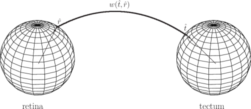
Figure 1: The cells of retina and tectum, which are assumed to be continuously distributed on unit spheres, are represented by their unit vectors $\hat{r}$ and $\hat{t}$, respectively. The two cell sheets are connected by positive connection weights $w(\hat{t},\hat{r})$.

According to the general reasoning in Ref. gpw1 we start with fixing the metric on the manifolds and determine the eigenfunctions of the corresponding Laplace-Beltrami operator. Afterwards, we expand the cooperativity functions with respect to these eigenfunctions and perform a linear analysis of the stationary uniform state.

II.1 Laplace-Beltrami Operator

For the time being we neglect the distinction between retina and tectum, because the following considerations are valid for both manifolds. Using spherical coordinates, we write the unit vector on the sphere as $\hat{x}=(\sin\vartheta\cos\varphi,\sin\vartheta\sin\varphi,\cos\vartheta)$. The Laplace-Beltrami operator on a manifold reads quite generally klein

$$\Delta=\frac{1}{\sqrt{g}}\,\partial_{\lambda}\left(g^{\lambda\mu}\sqrt{g}\,\partial_{\mu}\right)\,.$$ (4)

For the sphere the components of the covariant tensor $g_{\mu\nu}$ are

$$g_{11}=\left(\frac{\partial\hat{x}}{\partial\vartheta}\right)^{2}=1\,,\quad g_{12}=g_{21}=\frac{\partial\hat{x}}{\partial\vartheta}\,\frac{\partial\hat{x}}{\partial\varphi}=0\,,\quad g_{22}=\left(\frac{\partial\hat{x}}{\partial\varphi}\right)^{2}=\sin^{2}\vartheta\,.$$ (5)

With this the determinant of the covariant metric tensor reads $g=\sin^{2}\vartheta$ and the components of the contravariant metric are given by

$$g^{11}=1\,,\quad g^{12}=g^{21}=0\,,\quad g^{22}=\frac{1}{\sin^{2}\vartheta}\,,$$ (6)

whence the Laplace-Beltrami operator for the sphere takes the well-known form

$$\Delta_{\vartheta,\varphi}=\frac{1}{\sin\vartheta}\,\frac{\partial}{\partial\vartheta}\left(\sin\vartheta\frac{\partial}{\partial\vartheta}\right)+\frac{1}{\sin^{2}\vartheta}\frac{\partial^{2}}{\partial\varphi^{2}}\,.$$ (7)

Its eigenfunctions are known to be given by spherical harmonics $Y_{lm}(\hat{x})$:

$$\Delta_{\vartheta,\varphi}\,Y_{lm}(\hat{x})=-l(l+1)Y_{lm}(\hat{x})\,.$$ (8)

With $l=0,1,2,\ldots$ and $m=-l,-l+1,\ldots,l-1,l$ they are $(2l+1)$-fold degenerate and form a complete orthonormal system on the unit sphere:

$$\int\!\!d\Omega_{x}\,Y_{lm}(\hat{x}\,)Y_{l^{\prime}m^{\prime}}^{*}(\hat{x}\,) = \delta_{ll^{\prime}}\delta_{mm^{\prime}}\,,$$ (9)

$$\sum_{l=0}^{\infty}\sum_{m=-l}^{l}Y_{lm}(\hat{x}\,)Y_{lm}^{*}(\hat{x}^{\prime}\,) = \delta(\hat{x}-\hat{x}^{\prime})\,.$$ (10)

II.2 Cooperativity Functions

The argument of the cooperativity functions $c(\hat{x}\cdot\hat{x}^{\prime})$ is the scalar product $\hat{x}\cdot\hat{x}^{\prime}$ which takes values between $-1$ and $+1$. Therefore the cooperativity functions can be expanded in terms of Legendre functions $P_{l}(\hat{x}\cdot\hat{x}^{\prime})$, which form a complete orthogonal system on this interval (grad, , 7.221.1):

$$\int\limits_{-1}^{1}P_{l}(\sigma)P_{l^{\prime}}(\sigma)\,d\sigma = \frac{2}{2l+1}\,\delta_{ll^{\prime}}\,,$$ (11)

$$\frac{1}{2}\sum_{l=0}^{\infty}(2l+1)P_{l}(\sigma^{\prime})P_{l}(\sigma) = \delta(\sigma-\sigma^{\prime})\,.$$ (12)

Then the expansion of the cooperativity functions read

$$c(\hat{x}\cdot\hat{x}^{\prime})=\sum_{l=0}^{\infty}\frac{2l+1}{4\pi}f_{l}\,P_{l}(\hat{x}\cdot\hat{x}^{\prime})\,,$$ (13)

where $f_{l}$ denote the respective expansion coefficients. Using the Legendre addition theorem arf

$$P_{l}(\hat{x}\cdot\hat{x}^{\prime})=\frac{4\pi}{2l+1}\sum_{m=-l}^{l}Y_{lm}(\hat{x}\,)Y_{lm}^{*}(\hat{x}^{\prime})\,,$$ (14)

we arrive, for each manifold, at the expansion

$$c_{T}(\hat{t}\cdot\hat{t}^{\prime})=\sum_{L=0}^{\infty}\sum_{M=-L}^{L}f_{L}^{T}Y_{LM}^{T}(\hat{t}\,)Y_{LM}^{T*}(\hat{t}^{\prime}\,)\,,\quad c_{R}(\hat{r}\cdot\hat{r}^{\prime})=\sum_{l=0}^{\infty}\sum_{m=-l}^{l}f_{l}^{R}Y_{lm}^{R}(\hat{r})Y_{lm}^{R*}(\hat{r}^{\prime}\,)\,.$$ (15)

Note that the normalization of the cooperativity functions and the orthonormality relations (9) lead to the constraints $f_{0}^{T}=f_{0}^{R}=1$.

II.3 Eigenvalues

The initial state of ontogenesis with randomly distributed synaptic contacts is described by the stationary uniform solution of the generalized Häussler equations, $w_{0}(\hat{t},\hat{r})=1$. Its stability is analyzed by linearizing the Häussler equations (1) with respect to the deviation $v(\hat{t},\hat{r})=w(\hat{t},\hat{r})-w_{0}(\hat{t},\hat{r})$. The resulting linearized equations read

$$\dot{v}(\hat{t},\hat{r})=\hat{L}(\hat{t},\hat{r},v)$$ (16)

with the linear operator

$$\hskip 14.22636pt\hat{L}(\hat{t},\hat{r},v)=-\alpha v(\hat{t},\hat{r})-\frac{1}{8\pi}\int\!d\Omega_{t^{\prime}}\left[v(\hat{t}^{\prime},\hat{r})+\int\!d\Omega_{t^{\prime\prime}}\int\!d\Omega_{r^{\prime\prime}}\,c_{T}(\hat{t}^{\prime}\cdot\hat{t}^{\prime\prime})\,c_{R}(\hat{r}\cdot\hat{r}^{\prime\prime})\,v(\hat{t}^{\prime\prime},\hat{r}^{\prime\prime})\right]$$

$$-\frac{1}{8\pi}\int\!d\Omega_{r^{\prime}}\left[v(\hat{t},\hat{r}^{\prime})+\int\!d\Omega_{t^{\prime\prime}}\!\int\!d\Omega_{r^{\prime\prime}}\,c_{T}(\hat{t}\cdot\hat{t}^{\prime\prime})\,c_{R}(\hat{r}^{\prime}\cdot\hat{r}^{\prime\prime})\,v(\hat{t}^{\prime\prime},\hat{r}^{\prime\prime})\right]+\int\!d\Omega_{t^{\prime}}\!\int\!d\Omega_{r^{\prime}}\,c_{T}(\hat{t}\cdot\hat{t}^{\prime})\,c_{R}(\hat{r}\cdot\hat{r}^{\prime})\,v(\hat{t}^{\prime},\hat{r}^{\prime})\,.$$ (17)

To solve Eq. (16), we have to consider the eigenvalue problem of the linear operator (II.3). It has the eigenfunctions

$$v_{Ll}^{Mm}(\hat{t},\hat{r})=Y_{LM}^{T}(\hat{t}\,)Y_{lm}^{R}(\hat{r})$$ (18)

and the spectrum of eigenvalues reads gpw1 :

$$\Lambda_{Ll}^{Mm}=\left\{\begin{array}[]{cc}-\alpha-1&L=M=l=m=0\\ -\alpha+(f_{L}^{T}f_{l}^{R}-1)/2&L=M=0,\,(l,m)\not=(0,0)\\ &l=m=0,\,(L,M)\not=(0,0)\\ -\alpha+f_{L}^{T}f_{l}^{R}&\mbox{ otherwise }.\end{array}\right.$$ (19)

By changing the uniform growth rate $\alpha$ in a suitable way, the real parts of some eigenvalues (19) become positive and the system can be driven to the neighborhood of an instability. Which eigenvalues (19) become unstable in general depends on the respective values of the given expansion coefficients $f_{L}^{T}$, $f_{l}^{R}$. If we assume monotonically decreasing expansion coefficients $f_{L}^{T}$, $f_{l}^{R}$,

$$1=f_{0}^{T}\geq f_{1}^{T}\geq f_{2}^{T}\geq\cdots\geq 0\,,\qquad 1=f_{0}^{R}\geq f_{1}^{R}\geq f_{2}^{R}\geq\cdots\geq 0\,,$$ (20)

the maximum eigenvalue in (19) is given by $\Lambda_{\rm max}=\Lambda_{11}^{Mm}=-\alpha+f_{1}^{T}f_{1}^{R}$. Thus, the instability occurs when the global growth rate reaches its critical value $\alpha_{c}=f_{1}^{T}f_{1}^{R}$. At this instability point all nine modes with $(L^{u},l^{u})=(1,1)$ and $M^{u}=0,\pm 1$, $m^{u}=0,\pm 1$ become unstable, where we have introduced the index $u$ for the unstable modes.

III Nonlinear Analysis

In this section we specialize the generic order parameter equations of Ref. gpw1 to unit spheres. We observe that the quadratic term vanishes and derive selection rules for the appearance of cubic terms. Furthermore, we essentially simplify the calculation of the order parameter equations by taking into account the symmetry properties of the cubic terms. We show that the order parameter equations represent a potential dynamics, and determine the underlying potential.

III.1 General Structure of Order Parameter Equations

The linear stability analysis motivates treating the nonlinear Häussler equations (1) near the instability by decomposing the deviation $v(\hat{t},\hat{r})=w(\hat{t},\hat{r})-w_{0}(\hat{t},\hat{r})$ in unstable and stable contributions,

$$v(\hat{t},\hat{r})=U(\hat{t},\hat{r})+S(\hat{t},\hat{r})\,.$$ (21)

Using Einstein’s sum convention the expansion of the unstable modes reads

$$U(\hat{t},\hat{r})=U_{11}^{M^{u}m^{u}}Y_{1M^{u}}^{T}(\hat{t}\,)Y_{1m^{u}}^{R}(\hat{r}\,)\,,$$ (22)

and, correspondingly, the contribution of the stable modes is given by

$$S(\hat{t},\hat{r})=S_{Ll}^{Mm}Y_{LM}^{T}(\hat{t}\,)Y_{lm}^{R}(\hat{r}\,)\,.$$ (23)

Note that the summation in (23) is performed over all parameters $(L,l)$ except for $(L^{u},l^{u})=(1,1)$, i.e. from now on the parameters $(L,l)$ stand for the stable modes alone. With the help of the slaving principle of synergetics Haken1 ; Haken2 the original high-dimensional system can be reduced to a low-dimensional one which only contains the unstable amplitudes. The resulting order parameter equations read gpw1

$$\dot{U}^{M^{u}m^{u}} = \Lambda\,U^{M^{u}m^{u}}+A_{M^{u},M^{u}{}^{\prime}M^{u}{}^{\prime\prime}}^{m^{u},m^{u}{}^{\prime}m^{u}{}^{\prime\prime}}\,U^{M^{u}{}^{\prime}m^{u}{}^{\prime}}\,U^{M^{u}{}^{\prime\prime}m^{u}{}^{\prime\prime}}+B_{M^{u},M^{u}{}^{\prime}M^{u}{}^{\prime\prime}M^{u}{}^{\prime\prime\prime}}^{m^{u}{},m^{u}{}^{\prime}m^{u}{}^{\prime\prime}m^{u}{}^{\prime\prime\prime}}U^{M^{u}{}^{\prime}m^{u}{}^{\prime}}\,U^{M^{u}{}^{\prime\prime}m^{u}{}^{\prime\prime}}\,U^{M^{u}{}^{\prime\prime\prime}m^{u}{}^{\prime\prime\prime}}\,.$$ (24)

They contain, as usual, a linear, a quadratic, and a cubic term of the order parameters. The corresponding coefficients can be expressed in terms of the expansion coefficients $f_{L}^{T}$, $f_{l}^{R}$ of the cooperativity functions (15) and integrals over products of the eigenfunctions $Y_{lm}(\hat{x})$:

$$I_{l,l^{(1)}l^{(2)}\ldots l^{(n)}}^{m,m^{(1)}m^{(2)}\dots m^{(n)}} = \hskip 2.84526pt\int\!d\Omega_{x}\,Y_{lm}^{*}(\hat{x})\,Y_{l^{(1)}\,m^{(1)}}(\hat{x})\,Y_{l^{(2)}\,m^{(2)}}(\hat{x})\,\cdots\,Y_{l^{(n)}\,m^{(n)}}(\hat{x})\,,$$ (25)

$$J_{l^{(1)}l^{(2)}\ldots l^{(n)}}^{m^{(1)}m^{(2)}\ldots m^{(n)}} = \hskip 2.84526pt\int\!d\Omega_{x}\,Y_{l^{(1)}\,m^{(1)}}(\hat{x})\,Y_{l^{(2)}\,m^{(2)}}(\hat{x})\,\cdots\,Y_{l^{(n)}\,m^{(n)}}(\hat{x})\,.$$ (26)

The quadratic coefficients read

$$A_{M^{u},M^{u}{}^{\prime}M^{u}{}^{\prime\prime}}^{m^{u},m^{u}{}^{\prime}m^{u}{}^{\prime\prime}}=f_{1}^{T}\,f_{1}^{R}\,I_{1,1\,1}^{M^{u},M^{u}{}^{\prime}M^{u}{}^{\prime\prime}}\,I_{1,1\,1}^{m^{u},m^{u}{}^{\prime}m^{u}{}^{\prime\prime}}\,,$$ (27)

whereas the cubic coefficients are

$$B_{M^{u},M^{u}{}^{\prime}M^{u}{}^{\prime\prime}M^{u}{}^{\prime\prime\prime}}^{m^{u}{},m^{u}{}^{\prime}m^{u}{}^{\prime\prime}m^{u}{}^{\prime\prime\prime}} = -\frac{1}{8\pi}\,f_{1}^{T}\,f_{1}^{R}\left(I_{1,1\,1\,1}^{M^{u},M^{u}{}^{\prime}M^{u}{}^{\prime\prime}M^{u}{}^{\prime\prime\prime}}\,\delta_{m^{u}m^{u}{}^{\prime}}\,J_{1\,1}^{m^{u}{}^{\prime\prime}m^{u}{}^{\prime\prime\prime}}+I_{1,1\,1\,1}^{m^{u},m^{u}{}^{\prime}m^{u}{}^{\prime\prime}m^{u}{}^{\prime\prime\prime}}\delta_{M^{u}M^{u}{}^{\prime}}\,J_{1\,1}^{M^{u}{}^{\prime\prime}M^{u}{}^{\prime\prime\prime}}\right)$$ (28)

$$+\left\{\left[f_{L}^{T}\,f_{l}^{R}+f_{1}^{T}\,f_{1}^{R}\,\right]I_{1,1\,L}^{M^{u},M^{u}{}^{\prime}M}\,I_{1,1\,l}^{m^{u},m^{u}{}^{\prime}m}-\frac{1}{4\sqrt{\pi}}\,\left[\delta_{L0}\,\delta_{M0}\delta_{M^{u}M^{u}{}^{\prime}}\,\left(1+f_{l}^{R}\right)I_{1,1\,l}^{m^{u},m^{u}{}^{\prime}m}\right.\right.$$

$$\left.\left.+\delta_{l0}\,\delta_{m0}\delta_{m^{u}m^{u}{}^{\prime}}\,\left(1+f_{L}^{T}\right)\,I_{1,1\,L}^{M^{u},M^{u}{}^{\prime}M}\right]\right\}H_{Ll}^{Mm,M^{u}{}^{\prime\prime}m^{u}{}^{\prime\prime}M^{u}{}^{\prime\prime\prime}m^{u}{}^{\prime\prime\prime}}\,\,.$$

Note that Eq. (28) involves a summation over all stable modes $(L,M;l,m)$. As is common in synergetics, the cubic coefficients (28) consist in general of two parts, one stemming from the order parameters themselves and the other representing the influence of the center manifold $H$ on the order parameter dynamics according to

$$S_{Ll}^{Mm}=H_{Ll}^{Mm,M^{u}m^{u}M^{u}{}^{\prime}m^{u}{}^{\prime}}\,U^{M^{u}m^{u}}U^{M^{u}{}^{\prime}m^{u}{}^{\prime}}\,.$$ (29)

Here the center manifold coefficients $H_{Ll}^{Mm,M^{u}m^{u}M^{u}{}^{\prime}m^{u}{}^{\prime}}$ are defined by

$$H_{Ll}^{Mm,M^{u}m^{u}M^{u}{}^{\prime}m^{u}{}^{\prime}} = \frac{f_{1}^{T}f_{1}^{R}}{2\Lambda-\Lambda_{Ll}}\Bigg{[}I_{L,1\,1}^{M,M^{u}M^{u}{}^{\prime}}\,I_{l,1\,1}^{m,m^{u}m^{u}{}^{\prime}}-\frac{1}{4\sqrt{\pi}}\,\left(J_{1\,1}^{M^{u}M^{u}{}^{\prime}}\,I_{l,1\,1}^{m,m^{u}{}^{\prime}m^{u}{}^{\prime\prime}}\,\delta_{L0}\right.$$ (30)

$$\left.+J_{1\,1}^{m^{u}m^{u}{}^{\prime}}\,I_{L,1\,1}^{M,M^{u}M^{u}{}^{\prime}}\,\delta_{l0}\right)\Bigg{]}\,.$$

III.2 Integrals

The order parameter equations contain the following integrals: $J_{11}^{m^{\prime}m^{\prime\prime}},I_{1,11}^{m,m^{\prime}m^{\prime\prime}},I_{l,11}^{m,m^{\prime}m^{\prime\prime}},I_{1,1l}^{m,m^{\prime}m^{\prime\prime}},I_{1,111}^{m,m^{\prime}m^{\prime\prime}m^{\prime\prime\prime}}$. The first integral is obtained by the orthonormality relation (9) and

$$Y_{l-m}(\hat{x})=(-1)^{m}Y_{lm}^{*}(\hat{x})\,,$$ (31)

yielding $J_{11}^{m^{\prime}m^{\prime\prime}}=(-1)^{m^{\prime}}\delta_{m^{\prime},-m^{\prime\prime}}$. Integrals over three and four spherical harmonics can be calculated with the help of the following relation cohen :

$$Y_{l_{1},m_{1}}(\hat{x})Y_{l_{2},m_{2}}(\hat{x})=\sum_{l_{3}=|l_{1}-l_{2}|}^{l_{1}+l_{2}}\sum_{m_{3}=-l_{3}}^{l_{3}}\sqrt{\frac{(2l_{1}+1)(2l_{2}+1)}{4\pi(2l_{3}+1)}}\,C(l_{1},0,l_{2},0|l_{3},0)\,C(l_{1},m_{1},l_{2},m_{2}|l_{3},m_{3})\,Y_{l_{3},m_{3}}(\hat{x})\,,$$ (32)

where $C(l_{1},m_{1},l_{2},m_{2}|l_{3},m_{3})$ represent the Clebsch-Gordan coefficients heine . Applying (32) to integrals over three spherical harmonics leads to

$$I_{l,l^{\prime}l^{\prime\prime}}^{m,m^{\prime}m^{\prime\prime}}=\sqrt{\frac{(2l^{\prime}+1)(2l^{\prime\prime}+1)}{4\pi(2l+1)}}\,C(l^{\prime},0,l^{\prime\prime},0|l,0)\,C(l^{\prime},m^{\prime},l^{\prime\prime},m^{\prime\prime}|l,m)\,.$$ (33)

For $l^{\prime}=l^{\prime\prime}=1$ it follows

$$I_{l,11}^{m,m^{\prime}m^{\prime\prime}}=\frac{3}{\sqrt{4\pi(2l+1)}}\,C(1,0,1,0|l,0)\,C(1,m^{\prime},1,m^{\prime\prime}|l,m)\,.$$ (34)

As the Clebsch-Gordan coefficients $C(l_{1},0,l_{2},0|l_{3},0)$ vanish if the sum $l_{1}+l_{2}+l_{3}$ is odd heine , we obtain $I_{1,11}^{m,m^{\prime}m^{\prime\prime}}=0$. Thus, the quadratic contribution (27) to the order parameter equations (24) vanishes, by analogy with Euclidean manifolds gpw2 . Furthermore, non-vanishing integrals (34) can only occur for $l=0$ and $l=2$. For $l=0$ we obtain from the Clebsch-Gordan coefficients heine the result

$$I_{0,11}^{0,m^{\prime}m^{\prime\prime}}=\frac{(-1)^{m^{\prime}}}{\sqrt{4\pi}}\,\delta_{m^{\prime},m^{\prime\prime}}\,.$$ (35)

For $l=2$ we find, correspondingly, the nonvanishing integrals

$$I_{0,11}^{0,00}=\frac{1}{\sqrt{4\pi}}\,,\quad I_{2,11}^{0,00}=\frac{1}{\sqrt{5\pi}}\,,\quad I_{0,11}^{0,1-1}=I_{0,11}^{0,-11}=-\frac{1}{\sqrt{4\pi}}\,,\quad I_{2,11}^{0,1-1}=I_{2,11}^{0,-11}=\frac{1}{\sqrt{20\pi}}\,,$$

$$I_{2,11}^{1,10}=I_{2,11}^{1,01}=I_{2,11}^{-1,-10}=I_{2,11}^{-1,0-1}=\frac{3}{2\sqrt{15\pi}}\,,\quad I_{2,11}^{2,11}=\frac{3}{\sqrt{30\pi}}\,,\quad I_{2,11}^{-2,-1-1}=-\frac{3}{\sqrt{30\pi}}\,.$$ (36)

Furthermore, the integrals $I_{1,1l}^{m,m^{\prime}m^{\prime\prime}}$ follow from

$$I_{1,1l}^{m,m^{\prime}m^{\prime\prime}}=(-1)^{m^{\prime}+m^{\prime\prime}}I_{l,11}^{-m^{\prime\prime},-m\,m^{\prime}}\,.$$ (37)

Integrals over four spherical harmonics can also be calculated with the help of (32), and the result is

$$I_{l,l^{\prime}l^{\prime\prime}l^{\prime\prime\prime}}^{m,m^{\prime}m^{\prime\prime}m^{\prime\prime\prime}}=\sum_{l_{3}=|l^{\prime\prime}-l^{\prime\prime\prime}|}^{l^{\prime\prime}+l^{\prime\prime\prime}}\sum_{m_{3}=-l_{3}}^{l_{3}}\sqrt{\frac{(2l^{\prime\prime}+1)(2l^{\prime\prime\prime}+1)}{4\pi(2l_{3}+1)}}\,C(l^{\prime\prime},0,l^{\prime\prime\prime},0|l_{3},0)C(l^{\prime\prime},m^{\prime\prime},l^{\prime\prime\prime},m^{\prime\prime\prime}|l_{3},m_{3})I_{l,l^{\prime}l_{3}}^{m,m^{\prime}m_{3}}\,.$$ (38)

Specialyzing (38) to $l=l^{\prime}=l^{\prime\prime}=l^{\prime\prime\prime}=1$ and taking into account (33) leads to $I_{1,1\,1\,1}^{m,m^{\prime}m^{\prime\prime}m^{\prime\prime\prime}}\propto\delta_{m^{\prime}+m^{\prime\prime}+m^{\prime\prime\prime},m}$. Thus, we obtain the selection rule that the nonvanishing integrals $I_{1,1\,1\,1}^{m,m^{\prime}m^{\prime\prime}m^{\prime\prime\prime}}$ fulfill the condition $m^{\prime}+m^{\prime\prime}+m^{\prime\prime\prime}=m$. The detailed evaluation yields for those the respective values

$$I_{1,111}^{0,000} = \frac{9}{20\pi}\,,$$

$$I_{1,111}^{0,1-10}=I_{1,111}^{0,-110}=I_{1,111}^{0,10-1}=I_{1,111}^{0,-101}=I_{1,111}^{0,01-1}=I_{1,111}^{0,0-11} = -\frac{3}{20\pi}\,,$$

$$I_{1,111}^{1,100}=I_{1,111}^{1,010}=I_{1,111}^{1,001}=I_{1,111}^{-1,-100}=I_{1,111}^{-1,0-10}=I_{1,111}^{-1,00-1} = \frac{3}{20\pi}\,,$$

$$I_{1,111}^{1,11-1}=I_{1,111}^{1,1-11}=I_{1,111}^{1,-111}=I_{1,111}^{-1,1-1-1}=I_{1,111}^{-1,-11-1}=I_{1,111}^{-1,-1-11} = -\frac{3}{10\pi}\,.$$ (39)

III.3 Order Parameter Equations

To simplify the calculation of the cubic coefficients (28) in the order parameter equations (24), we perform some basic considerations which lead to helpful symmetry properties. To this end we start with replacing $m^{u}$ by $-m^{u}$. Using Eq. (31) we obtain $I_{1,1\,1\,1}^{m^{u},m^{u^{\prime}}m^{u^{\prime\prime}}m^{u^{\prime\prime\prime}}}=I_{1,1\,1\,1}^{-m^{u},-m^{u^{\prime}}-m^{u^{\prime\prime}}-m^{u^{\prime\prime\prime}}}$. Corresponding symmetry relations can also be derived for the other terms in (28). Therefore, we conclude that the order parameter equation for $U^{-M^{u}-m^{u}}$ is obtained from that of $U^{M^{u}m^{u}}$ by negating all indices $M^{u}$ and $m^{u}$ with unchanged factors. Thus, instead of explicitly calculating nine order parameter equations, it is sufficient to restrict oneself determining the order parameter equations for $U^{00}$, $U^{10}$, $U^{01}$, and $U^{11}$. The remaining five order parameter equations follow instantaneously from those by applying the symmetry relations. With this the order parameter equations result in

$$\dot{U}^{00} = \Lambda U^{00}+\beta_{1}(U^{00})^{3}-2\beta_{2}U^{00}U^{-10}U^{10}-2\bar{\beta}_{2}U^{00}U^{0-1}U^{01}+2\beta_{3}U^{00}U^{1-1}U^{-11}+2\beta_{3}U^{00}U^{-1-1}U^{11}$$

$$+\beta_{4}U^{01}U^{10}U^{-1-1}+\beta_{4}U^{0-1}U^{-10}U^{11}+\beta_{4}U^{0-1}U^{10}U^{-11}+\beta_{4}U^{01}U^{-10}U^{1-1}\,,$$

$$\dot{U}^{11} = \Lambda U^{11}+\beta_{4}U^{00}U^{01}U^{10}+\beta_{5}(U^{01})^{2}U^{1-1}+\beta_{6}U^{01}U^{0-1}U^{11}+\beta_{3}(U^{00})^{2}U^{11}$$

$$+\beta_{5}(U^{10})^{2}U^{-11}+\bar{\beta}_{6}U^{10}U^{-10}U^{11}+\beta_{7}U^{11}U^{1-1}U^{-11}+\beta_{8}(U^{11})^{2}U^{-1-1}\,,$$

$$\dot{U}^{-1-1} = \Lambda U^{-1-1}+\beta_{4}U^{00}U^{0-1}U^{-10}+\beta_{5}(U^{0-1})^{2}U^{-11}+\beta_{6}U^{0-1}U^{01}U^{-1-1}+\beta_{3}(U^{00})^{2}U^{-1-1}$$

$$+\beta_{5}(U^{-10})^{2}U^{1-1}+\bar{\beta}_{6}U^{-10}U^{10}U^{-1-1}+\beta_{7}U^{-1-1}U^{-11}U^{1-1}+\beta_{8}(U^{-1-1})^{2}U^{11}\,,$$

$$\dot{U}^{1-1} = \Lambda U^{1-1}+\beta_{4}U^{00}U^{0-1}U^{10}+\beta_{5}(U^{0-1})^{2}U^{11}+\beta_{6}U^{0-1}U^{01}U^{1-1}+\beta_{3}(U^{00})^{2}U^{1-1}$$

$$+\beta_{5}(U^{10})^{2}U^{-1-1}+\bar{\beta}_{6}U^{10}U^{-10}U^{1-1}+\beta_{7}U^{1-1}U^{11}U^{-1-1}+\beta_{8}(U^{1-1})^{2}U^{-11}\,,$$

$$\dot{U}^{-11} = \Lambda U^{-11}+\beta_{4}U^{00}U^{01}U^{-10}+\beta_{5}(U^{01})^{2}U^{-1-1}+\beta_{6}U^{01}U^{0-1}U^{-11}+\beta_{3}(U^{00})^{2}U^{-11}$$

$$+\beta_{5}(U^{-10})^{2}U^{11}+\bar{\beta}_{6}U^{-10}U^{10}U^{-11}+\beta_{7}U^{-11}U^{-1-1}U^{11}+\beta_{8}(U^{-11})^{2}U^{1-1}\,,$$

$$\dot{U}^{01} = \Lambda U^{01}+\bar{\beta}_{2}U^{01}(U^{00})^{2}+\beta_{9}(U^{01})^{2}U^{0-1}-2\beta_{3}U^{01}U^{10}U^{-10}-\beta_{4}U^{00}U^{11}U^{-10}$$

$$-\beta_{4}U^{00}U^{10}U^{-11}-\beta_{6}U^{01}U^{11}U^{-1-1}-\beta_{6}U^{01}U^{1-1}U^{-11}-2\beta_{5}U^{0-1}U^{11}U^{-11}\,,$$

$$\dot{U}^{0-1} = \Lambda U^{0-1}+\bar{\beta}_{2}U^{0-1}(U^{00})^{2}+\beta_{9}(U^{0-1})^{2}U^{01}-2\beta_{3}U^{0-1}U^{-10}U^{10}-\beta_{4}U^{00}U^{-1-1}U^{10}$$

$$-\beta_{4}U^{00}U^{-10}U^{1-1}-\beta_{6}U^{0-1}U^{-1-1}U^{11}-\beta_{6}U^{0-1}U^{-11}U^{1-1}-2\beta_{5}U^{01}U^{-1-1}U^{1-1}\,,$$

$$\dot{U}^{10} = \Lambda U^{10}+\beta_{2}U^{10}(U^{00})^{2}+\bar{\beta}_{9}(U^{10})^{2}U^{-10}-2\beta_{3}U^{10}U^{01}U^{0-1}-\beta_{4}U^{00}U^{11}U^{0-1}$$

$$-\beta_{4}U^{00}U^{01}U^{1-1}-\bar{\beta}_{6}U^{10}U^{11}U^{-1-1}-\bar{\beta}_{6}U^{10}U^{-11}U^{1-1}-2\beta_{5}U^{-10}U^{11}U^{1-1}\,,$$

$$\dot{U}^{-10} = \Lambda U^{-10}+\beta_{2}U^{-10}(U^{00})^{2}+\bar{\beta}_{9}(U^{-10})^{2}U^{10}-2\beta_{3}U^{-10}U^{0-1}U^{01}-\beta_{4}U^{00}U^{-1-1}U^{01}$$ (40)

$$-\beta_{4}U^{00}U^{0-1}U^{-11}-\bar{\beta}_{6}U^{-10}U^{-1-1}U^{11}-\bar{\beta}_{6}U^{-10}U^{1-1}U^{-11}-2\beta_{5}U^{10}U^{-1-1}U^{-11}\,.$$

With the abbreviations $\tilde{\gamma}=\gamma/\pi^{2}$, $\gamma=f_{1}^{T}f_{1}^{R}$ and $\gamma^{L,l}=f_{L}^{T}f_{l}^{R}$ the respective coefficients in (40) read

$$\beta_{1} = -\frac{9}{80}\tilde{\gamma}+\frac{\tilde{\gamma}}{80}\frac{2\gamma+\gamma^{2,0}-1}{2\gamma-\alpha-(\gamma^{2,0}-1)/2}+\frac{\tilde{\gamma}}{80}\frac{2\gamma+\gamma^{0,2}-1}{2\gamma-\alpha-(\gamma^{0,2}-1)/2}+\frac{\tilde{\gamma}}{25}\frac{\gamma+\gamma^{2,2}}{2\gamma-\alpha-\gamma^{2,2}}\,,$$

$$\beta_{2} = -\frac{9}{80}\tilde{\gamma}-\frac{\tilde{\gamma}}{40}\frac{2\gamma+\gamma^{2,0}-1}{2\gamma-\alpha-(\gamma^{2,0}-1)/2}+\frac{\tilde{\gamma}}{80}\frac{2\gamma+\gamma^{0,2}-1}{2\gamma-\alpha-(\gamma^{0,2}-1)/2}-\frac{2\tilde{\gamma}}{25}\frac{\gamma+\gamma^{2,2}}{2\gamma-\alpha-\gamma^{2,2}}\,,$$

$$\bar{\beta}_{2} = -\frac{9}{80}\tilde{\gamma}+\frac{\tilde{\gamma}}{80}\frac{2\gamma+\gamma^{2,0}-1}{2\gamma-\alpha-(\gamma^{2,0}-1)/2}-\frac{\tilde{\gamma}}{40}\frac{2\gamma+\gamma^{0,2}-1}{2\gamma-\alpha-(\gamma^{0,2}-1)/2}-\frac{2\tilde{\gamma}}{25}\frac{\gamma+\gamma^{2,2}}{2\gamma-\alpha-\gamma^{2,2}}\,,$$

$$\beta_{3} = -\frac{3}{80}\tilde{\gamma}-\frac{\tilde{\gamma}}{160}\frac{2\gamma+\gamma^{2,0}-1}{2\gamma-\alpha-(\gamma^{2,0}-1)/2}-\frac{\tilde{\gamma}}{160}\frac{2\gamma+\gamma^{0,2}-1}{2\gamma-\alpha-(\gamma^{0,2}-1)/2}+\frac{11\tilde{\gamma}}{200}\frac{\gamma+\gamma^{2,2}}{2\gamma-\alpha-\gamma^{2,2}}\,,$$

$$\beta_{4} = -\frac{3}{40}\tilde{\gamma}-\frac{3\tilde{\gamma}}{160}\frac{2\gamma+\gamma^{2,0}-1}{2\gamma-\alpha-(\gamma^{2,0}-1)/2}-\frac{3\tilde{\gamma}}{160}\frac{2\gamma+\gamma^{0,2}-1}{2\gamma-\alpha-(\gamma^{0,2}-1)/2}+\frac{21\tilde{\gamma}}{200}\frac{\gamma+\gamma^{2,2}}{2\gamma-\alpha-\gamma^{2,2}}\,,$$

$$\beta_{5} = \frac{3}{40}\tilde{\gamma}+\frac{3\tilde{\gamma}}{160}\frac{2\gamma+\gamma^{2,0}-1}{2\gamma-\alpha-(\gamma^{2,0}-1)/2}+\frac{3\tilde{\gamma}}{160}\frac{2\gamma+\gamma^{0,2}-1}{2\gamma-\alpha-(\gamma^{0,2}-1)/2}-\frac{3\tilde{\gamma}}{200}\frac{\gamma+\gamma^{2,2}}{2\gamma-\alpha-\gamma^{2,2}}\,,$$

$$\beta_{6} = \frac{3}{20}\tilde{\gamma}+\frac{\tilde{\gamma}}{32}\frac{2\gamma+\gamma^{2,0}-1}{2\gamma-\alpha-(\gamma^{2,0}-1)/2}-\frac{\tilde{\gamma}}{160}\frac{2\gamma+\gamma^{0,2}-1}{2\gamma-\alpha-(\gamma^{0,2}-1)/2}-\frac{13\tilde{\gamma}}{200}\frac{\gamma+\gamma^{2,2}}{2\gamma-\alpha-\gamma^{2,2}}\,,$$

$$\bar{\beta}_{6} = \frac{3}{20}\tilde{\gamma}-\frac{\tilde{\gamma}}{160}\frac{2\gamma+\gamma^{2,0}-1}{2\gamma-\alpha-(\gamma^{2,0}-1)/2}+\frac{\tilde{\gamma}}{32}\frac{2\gamma+\gamma^{0,2}-1}{2\gamma-\alpha-(\gamma^{0,2}-1)/2}-\frac{13\tilde{\gamma}}{200}\frac{\gamma+\gamma^{2,2}}{2\gamma-\alpha-\gamma^{2,2}}\,,$$

$$\beta_{7} = -\frac{3}{10}\tilde{\gamma}-\frac{\tilde{\gamma}}{32}\frac{2\gamma+\gamma^{2,0}-1}{2\gamma-\alpha-(\gamma^{2,0}-1)/2}-\frac{\tilde{\gamma}}{32}\frac{2\gamma+\gamma^{0,2}-1}{2\gamma-\alpha-(\gamma^{0,2}-1)/2}-\frac{11\tilde{\gamma}}{200}\frac{\gamma+\gamma^{2,2}}{2\gamma-\alpha-\gamma^{2,2}}\,,$$

$$\beta_{8} = -\frac{3}{20}\tilde{\gamma}+\frac{\tilde{\gamma}}{160}\frac{2\gamma+\gamma^{2,0}-1}{2\gamma-\alpha-(\gamma^{2,0}-1)/2}+\frac{\tilde{\gamma}}{160}\frac{2\gamma+\gamma^{0,2}-1}{2\gamma-\alpha-(\gamma^{0,2}-1)/2}+\frac{19\tilde{\gamma}}{200}\frac{\gamma+\gamma^{2,2}}{2\gamma-\alpha-\gamma^{2,2}}\,,$$

$$\beta_{9} = \frac{9}{40}\tilde{\gamma}-\frac{\tilde{\gamma}}{40}\frac{2\gamma+\gamma^{2,0}-1}{2\gamma-\alpha-(\gamma^{2,0}-1)/2}+\frac{\tilde{\gamma}}{80}\frac{2\gamma+\gamma^{0,2}-1}{2\gamma-\alpha-(\gamma^{0,2}-1)/2}+\frac{\tilde{\gamma}}{25}\frac{\gamma+\gamma^{2,2}}{2\gamma-\alpha-\gamma^{2,2}}\,,$$

$$\bar{\beta}_{9} = \frac{9}{40}\tilde{\gamma}+\frac{\tilde{\gamma}}{80}\frac{2\gamma+\gamma^{2,0}-1}{2\gamma-\alpha-(\gamma^{2,0}-1)/2}-\frac{\tilde{\gamma}}{40}\frac{2\gamma+\gamma^{0,2}-1}{2\gamma-\alpha-(\gamma^{0,2}-1)/2}+\frac{\tilde{\gamma}}{25}\frac{\gamma+\gamma^{2,2}}{2\gamma-\alpha-\gamma^{2,2}}\,.$$ (41)

The first term proportional to $\tilde{\gamma}$ describes the influence of the order parameters themselves, while the other terms stand for the contributions of the center manifold.

III.4 Real Variables

To investigate how the complex order parameter equations contribute to the one-to-one retinotopy, we transform them to real variables according to

$$\begin{array}[]{rclcrclcrcl}\vspace{0.2cm}u_{0}&=&U^{00}/\sqrt{2}&,&u_{1}&=&(U^{11}+U^{-1-1})/2&,&u_{2}&=&i(U^{11}-U^{-1-1})/2\\ \vspace{0.2cm}u_{3}&=&(U^{1-1}+U^{-11})/2&,&u_{4}&=&i(U^{1-1}-U^{-11})/2&,&u_{5}&=&(U^{01}-U^{0-1})/2\\ u_{6}&=&i(U^{01}+U^{0-1})/2&,&u_{7}&=&(U^{10}-U^{-10})/2&,&u_{8}&=&i(U^{10}+U^{-10})/2\,.\end{array}$$ (42)

Then the equations of evolution for the real variables $u_{i}$ read

$$\dot{u}_{0} = \Lambda u_{0}+2\beta_{1}u_{0}^{3}+2\bar{\beta}_{2}u_{0}(u_{5}^{2}+u_{6}^{2})+2\beta_{2}u_{0}(u_{7}^{2}+u_{8}^{2})+2\beta_{3}u_{0}(u_{1}^{2}+u_{2}^{2}+u_{3}^{2}+u_{4}^{2})$$ (43)

$$+\sqrt{2}\,\beta_{4}(u_{1}u_{5}u_{7}+u_{2}u_{5}u_{8}+u_{2}u_{6}u_{7}+u_{4}u_{6}u_{7}-u_{1}u_{6}u_{8}-u_{3}u_{5}u_{7}-u_{4}u_{5}u_{8}-u_{3}u_{6}u_{8})\,,$$

$$\dot{u}_{1} = \Lambda u_{1}+\sqrt{2}\,\beta_{4}u_{0}(u_{5}u_{7}-u_{6}u_{8})+\beta_{5}(u_{3}u_{5}^{2}-u_{3}u_{6}^{2}-2u_{4}u_{5}u_{6})-\beta_{6}u_{1}(u_{5}^{2}+u_{6}^{2})-\bar{\beta}_{6}u_{1}(u_{7}^{2}+u_{8}^{2})$$ (44)

$$+2\beta_{3}u_{0}^{2}u_{1}+\beta_{5}(u_{3}u_{7}^{2}-u_{3}u_{8}^{2}+2u_{4}u_{7}u_{8})+\beta_{7}u_{1}(u_{3}^{2}+u_{4}^{2})+\beta_{8}u_{1}(u_{1}^{2}+u_{2}^{2})\,,$$

$$\dot{u}_{2} = \Lambda u_{2}+\sqrt{2}\,\beta_{4}u_{0}(u_{5}u_{8}+u_{6}u_{7})+\beta_{5}(u_{5}^{2}u_{4}-u_{4}u_{6}^{2}+2u_{3}u_{5}u_{6})-\beta_{6}u_{2}(u_{5}^{2}+u_{6}^{2})-\bar{\beta}_{6}u_{2}(u_{7}^{2}+u_{8}^{2})$$ (45)

$$+2\beta_{3}u_{0}^{2}u_{2}-\beta_{5}(u_{4}u_{7}^{2}-u_{4}u_{8}^{2}-2u_{3}u_{7}u_{8})+\beta_{7}u_{2}(u_{3}^{2}+u_{4}^{2})+\beta_{8}u_{2}(u_{1}^{2}+u_{2}^{2})\,,$$

$$\dot{u}_{3} = \Lambda u_{3}-\sqrt{2}\,\beta_{4}u_{0}(u_{5}u_{7}+u_{6}u_{8})+\beta_{5}(u_{1}u_{5}^{2}-u_{1}u_{6}^{2}+2u_{2}u_{5}u_{6})-\beta_{6}u_{3}(u_{5}^{2}+u_{6}^{2})-\bar{\beta}_{6}u_{3}(u_{7}^{2}+u_{8}^{2})$$ (46)

$$+2\beta_{3}u_{0}^{2}u_{3}+\beta_{5}(u_{1}u_{7}^{2}-u_{1}u_{8}^{2}+2u_{2}u_{7}u_{8})+\beta_{7}u_{3}(u_{1}^{2}+u_{2}^{2})+\beta_{8}u_{3}(u_{3}^{2}+u_{4}^{2})\,,$$

$$\dot{u}_{4} = \Lambda u_{4}+\sqrt{2}\,\beta_{4}u_{0}(u_{6}u_{7}-u_{5}u_{8})+\beta_{5}(u_{2}u_{5}^{2}-u_{2}u_{6}^{2}-2u_{1}u_{5}u_{6})-\beta_{6}u_{4}(u_{5}^{2}+u_{6}^{2})-\bar{\beta}_{6}u_{4}(u_{7}^{2}+u_{8}^{2})$$ (47)

$$+2\beta_{3}u_{0}^{2}u_{4}+\beta_{5}(u_{2}u_{8}^{2}-u_{2}u_{7}^{2}+2u_{1}u_{7}u_{8})+\beta_{7}u_{4}(u_{1}^{2}+u_{2}^{2})+\beta_{8}u_{4}(u_{3}^{2}+u_{4}^{2})\,,$$

$$\dot{u}_{5} = \Lambda u_{5}+2\bar{\beta}_{2}u_{0}^{2}u_{5}-\beta_{9}u_{5}(u_{5}^{2}+u_{6}^{2})+2\beta_{3}u_{5}(u_{7}^{2}+u_{8}^{2})+\sqrt{2}\,\beta_{4}u_{0}(u_{1}u_{7}-u_{3}u_{7}+u_{2}u_{8}-u_{4}u_{8})$$ (48)

$$-\beta_{6}u_{5}(u_{1}^{2}+u_{2}^{2}+u_{3}^{2}+u_{4}^{2})-2\beta_{5}(u_{1}u_{4}u_{6}-u_{1}u_{3}u_{5}-u_{2}u_{4}u_{5}-u_{2}u_{3}u_{6})\,,$$

$$\dot{u}_{6} = \Lambda u_{6}+2\bar{\beta}_{2}u_{0}^{2}u_{6}-\beta_{9}u_{6}(u_{5}^{2}+u_{6}^{2})+2\beta_{3}u_{6}(u_{7}^{2}+u_{8}^{2})+\sqrt{2}\,\beta_{4}u_{0}(u_{2}u_{7}+u_{4}u_{7}-u_{1}u_{8}-u_{3}u_{8})$$ (49)

$$-\beta_{6}u_{6}(u_{1}^{2}+u_{2}^{2}+u_{3}^{2}+u_{4}^{2})-2\beta_{5}(u_{1}u_{4}u_{5}+u_{1}u_{3}u_{6}+u_{2}u_{4}u_{6}-u_{2}u_{3}u_{5})\,,$$

$$\dot{u}_{7} = \Lambda u_{7}+2\beta_{2}u_{0}^{2}u_{7}-\bar{\beta}_{9}u_{7}(u_{7}^{2}+u_{8}^{2})+2\beta_{3}u_{7}(u_{5}^{2}+u_{6}^{2})+\sqrt{2}\,\beta_{4}u_{0}(u_{1}u_{5}-u_{3}u_{5}+u_{2}u_{6}+u_{4}u_{6})$$ (50)

$$-\bar{\beta}_{6}u_{7}(u_{1}^{2}+u_{2}^{2}+u_{3}^{2}+u_{4}^{2})-2\beta_{5}(u_{2}u_{4}u_{7}-u_{1}u_{3}u_{7}-u_{2}u_{3}u_{8}-u_{1}u_{4}u_{8})\,,$$

$$\dot{u}_{8} = \Lambda u_{8}+2\beta_{2}u_{0}^{2}u_{8}-\bar{\beta}_{9}u_{8}(u_{7}^{2}+u_{8}^{2})+2\beta_{3}u_{8}(u_{5}^{2}+u_{6}^{2})-\sqrt{2}\,\beta_{4}u_{0}(u_{1}u_{6}+u_{3}u_{6}-u_{2}u_{5}+u_{4}u_{5})$$ (51)

$$-\bar{\beta}_{6}u_{8}(u_{1}^{2}+u_{2}^{2}+u_{3}^{2}+u_{4}^{2})-2\beta_{5}(u_{1}u_{3}u_{8}-u_{2}u_{3}u_{7}-u_{1}u_{4}u_{7}-u_{2}u_{4}u_{8})\,.$$

Note that the real order parameter equations (43)–(51) follow according to

$$\dot{u}_{i}=-\frac{\partial V(\{u_{j}\})}{\partial u_{i}}$$ (52)

from the potential

$$V(\{u_{j}\}) = -\frac{\Lambda}{2}\sum_{j=0}^{8}u_{j}^{2}-\frac{\beta_{1}}{2}u_{0}^{4}-\bar{\beta}_{2}u_{0}^{2}(u_{5}^{2}+u_{6}^{2})-\beta_{2}u_{0}^{2}(u_{7}^{2}+u_{8}^{2})-\beta_{3}u_{0}^{2}(u_{1}^{2}+u_{2}^{2}+u_{3}^{2}+u_{4}^{2})$$ (53)

$$-\sqrt{2}\beta_{4}u_{0}(u_{1}u_{5}u_{7}+u_{2}u_{5}u_{8}+u_{2}u_{6}u_{7}+u_{4}u_{6}u_{7}-u_{1}u_{6}u_{8}-u_{3}u_{5}u_{7}-u_{4}u_{5}u_{8}-u_{3}u_{6}u_{8})$$

$$-\beta_{5}(u_{5}^{2}-u_{6}^{2})(u_{1}u_{3}+u_{2}u_{4})-\beta_{5}(u_{7}^{2}-u_{8}^{2})(u_{1}u_{3}-u_{2}u_{4})-2\beta_{5}u_{7}u_{8}(u_{1}u_{4}+u_{2}u_{3})$$

$$-2\beta_{5}u_{5}u_{6}(u_{2}u_{3}-u_{1}u_{4})+\frac{1}{2}[\beta_{6}(u_{5}^{2}+u_{6}^{2})+\bar{\beta}_{6}(u_{7}^{2}+u_{8}^{2})](u_{1}^{2}+u_{2}^{2}+u_{3}^{2}+u_{4}^{2})-\frac{\beta_{7}}{2}(u_{1}^{2}+u_{2}^{2})(u_{3}^{2}+u_{4}^{2})$$

$$-\beta_{3}(u_{5}^{2}+u_{6}^{2})(u_{7}^{2}+u_{8}^{2})-\frac{\beta_{8}}{4}\left[(u_{1}^{2}+u_{2}^{2})^{2}+(u_{3}^{2}+u_{4}^{2})^{2}\right]+\frac{\beta_{9}}{4}(u_{5}^{2}+u_{6}^{2})^{2}+\frac{\bar{\beta}_{9}}{4}(u_{7}^{2}+u_{8}^{2})^{2}\,.$$

Naturally, a complete analytical determination of all stationary states of the real order parameter equations (43)–(51) is impossible. However, we are able to demonstrate that certain stationary states admit for retinotopic modes.

III.5 Special Case

To this end we consider the special case $u_{1},u_{2},u_{5},u_{6},u_{7},u_{8}=0$. Then the equations (43), (46), and (47) for the non-vanishing amplitudes $u_{0}$, $u_{3}$, $u_{4}$ reduce to

$$\dot{u}_{0} = \Lambda u_{0}+2\beta_{1}u_{0}^{3}+2\beta_{3}(u_{3}^{2}+u_{4}^{2})u_{0}\,,$$

$$\dot{u}_{3} = \Lambda u_{3}+2\beta_{3}u_{0}^{2}u_{3}+\beta_{8}(u_{3}^{2}+u_{4}^{2})u_{3}\,,$$

$$\dot{u}_{4} = \Lambda u_{4}+2\beta_{3}u_{0}^{2}u_{4}+\beta_{8}(u_{3}^{2}+u_{4}^{2})u_{4}\,.$$ (54)

Due to the relation

$$\frac{\dot{u}_{3}}{u_{3}}=\frac{\dot{u}_{4}}{u_{4}}$$ (55)

one obtains constant phase-shift angles, i.e. it holds $u_{3}\propto u_{4}$. Therefore, the system of three coupled differential equations can be reduced to two variables. To this end we introduce the new variable

$$\xi=\sqrt{u_{3}^{2}+u_{4}^{2}}\,,$$ (56)

which leads to

$$\dot{u}_{0} = \Lambda u_{0}+2\beta_{1}u_{0}^{3}+2\beta_{3}\xi^{2}u_{0}\,,$$

$$\dot{\xi} = \Lambda\xi+2\beta_{3}u_{0}^{2}\xi+\beta_{8}\xi^{3}\,.$$ (57)

The stationary solution, which corresponds to a coexistence of the two modes, is given by

$$u_{0}^{2}=-\frac{\Lambda}{2(\beta_{3}+\beta_{8})}\,,\quad\xi^{2}=-\frac{\Lambda}{\beta_{3}+\beta_{8}}\,,$$ (58)

where we used the relation $\beta_{8}=\beta_{1}+\beta_{3}$ following from (41). Demanding real amplitudes $u_{0}$, $\xi$ leads to the coexistence condition

$$\beta_{3}+\beta_{8}<0\,.$$ (59)

Furthermore, we require stability for this state. Therefore we consider the corresponding potential $V(u_{0},\xi)$, which can be read off from (53) and (56):

$$V(u_{0},\xi)=-\frac{\Lambda}{2}(u_{0}^{2}+\xi^{2})-\frac{\beta_{1}}{2}u_{0}^{4}-\beta_{3}u_{0}^{2}\xi^{2}-\frac{\beta_{4}}{4}\xi^{4}\,.$$ (60)

Stable states correspond to a minimum of $V$, which leads to the conditions

$$2\beta_{3}-\beta_{8}>0\,,\quad\beta_{3}-\beta_{8}>0\,.$$ (61)

The inequalities (59), (61) can be summarized according to

$$\beta_{8}<0\,,\quad\beta_{3}<-\beta_{8}\,,\quad 2\beta_{3}>\beta_{8}\,.$$ (62)

If they are valid, both the $u_{0}$- and the $\xi$-mode coexist. If we set $u_{4}=0$, without loss of generality, the solution reads in complex variables according to (56)

$$U^{00}=\sqrt{-\frac{\Lambda}{\beta_{3}+\beta_{8}}}\,,\qquad U^{1-1}=U^{-11}=-\sqrt{-\frac{\Lambda}{\beta_{3}+\beta_{8}}}\,.$$ (63)

Thus, the unstable part (22) is given by

$$U(\hat{t},\hat{r})=\sqrt{-\frac{\Lambda}{\beta_{3}+\beta_{8}}}\,\Big{[}Y_{10}^{T}(\hat{t}\,)Y_{10}^{R}(\hat{r})-Y_{11}^{T}(\hat{t}\,)Y_{1-1}^{R}(\hat{r})-Y_{1-1}^{T}(\hat{t}\,)Y_{11}^{R}(\hat{r})\Big{]}\,.$$ (64)

Using the Legendre addition theorem (14) reduces (64) to

$$U(\hat{t},\hat{r})=\sqrt{-\frac{\Lambda}{\beta_{3}+\beta_{8}}}\,P_{1}(\hat{t}\cdot\hat{r})$$ (65)

with $P_{1}(\hat{t}\cdot\hat{r})=\hat{t}\cdot\hat{r}$. Thus, the unstable part is minimal, if $\hat{t}$ and $\hat{r}$ are antiparallel, i.e. the distance of the corresponding points on the unit sphere is maximum. Decreasing of the angle between $\hat{t}$ and $\hat{r}$ leads to increasing values of $U(\hat{t},\hat{r})$, and the maximum occurs for parallel unit vectors. This justifies calling the mode (65) retinotopic.

IV One-to-One Retinotopy

Now we investigate whether the generalized Häussler equations (1) describe the emergence of a perfect one-to-one retinotopy between two spheres. To this end we follow the unpublished suggestions of Ref. Malsburg4 and treat systematically the contribution of higher modes. Because the Legendre functions form a complete orthogonal system (11), (12) for functions defined on the interval $[-1,+1]$, their products can always be written as linear combinations of Legendre functions. This motivates that the influence of higher modes upon the connection weights, which obey the generalized Häussler equations (1), can be included by the ansatz

$$w(\sigma)=\sum_{l=0}^{\infty}(2l+1)Z_{l}P_{l}(\sigma)\,,$$ (66)

where the amplitudes $Z_{l}$ are time dependent.

IV.1 Recursion Relations

Inserting (66) into the generalized Häussler equations (1) and performing the integrals over the respective unit spheres leads to

$$\sum_{l=0}^{\infty}(2l+1)\dot{Z}_{l}P_{l}(\sigma)=\alpha\left[1-\sum_{l=0}^{\infty}(2l+1)Z_{l}P_{l}(\sigma)\right]+\sum_{l=0}^{\infty}(2l+1)Z_{l}P_{l}(\sigma)\sum_{l^{\prime}=0}^{\infty}(2l^{\prime}+1)Z_{l^{\prime}}f_{l^{\prime}}^{T}f_{l^{\prime}}^{R}[P_{l^{\prime}}(\sigma)-Z_{l^{\prime}}]\,.$$ (67)

The products of Legendre functions occuring in (67) can be reduced to linear combinations of single Legendre functions according to the standard decomposition (grad, , 8.915)

$$P_{l}(\sigma)P_{l^{\prime}}(\sigma)=\sum_{k=0}^{l}A_{l,l^{\prime},k}P_{l+l^{\prime}-2k}(\sigma)\,,\quad l\leq l^{\prime}$$ (68)

with the coefficients

$$A_{l,l^{\prime},k}=\frac{(2l^{\prime}+2l-4k+1)\,a_{l^{\prime}-k}a_{k}a_{l-k}}{(2l^{\prime}+2l-2k+1)\,a_{l+l^{\prime}-k}}\,,\quad a_{k}=\frac{(2k-1)!!}{k!}\,.$$ (69)

Thus, contributions to the polynomial $P_{\tilde{l}}(\sigma)$ only occur iff the relation $k=(l+l^{\prime}-\tilde{l})/2$ is fulfilled. Furthermore, using the orthonormality relation (11) yields the following recursion relation for the amplitudes $Z_{l}$:

$$(2l+1)\dot{Z}_{l} = \alpha[\delta_{l,0}-(2l+1)Z_{l}]-(2l+1)Z_{l}(Z_{0}^{2}+3f_{1}^{T}f_{1}^{R}Z_{1}^{2})+\sum_{l^{\prime}=0}^{\infty}(2l^{\prime}+1)Z_{l^{\prime}}\left[\sum_{l^{\prime\prime}=0}^{l}(2l^{\prime\prime}+1)Z_{l^{\prime\prime}}f_{l^{\prime\prime}}^{T}f_{l^{\prime\prime}}^{R}\right.$$ (70)

$$\left.\times\sum_{k=0}^{l^{\prime\prime}}A_{l^{\prime},l^{\prime\prime},k}\delta_{k,(l^{\prime}+l^{\prime\prime}-l)/2}+\sum_{l^{\prime\prime}=l^{\prime}+1}^{\infty}(2l^{\prime\prime}+1)Z_{l^{\prime\prime}}f_{l^{\prime\prime}}^{T}f_{l^{\prime\prime}}^{R}\sum_{k=0}^{l^{\prime}}A_{l^{\prime},l^{\prime\prime},k}\delta_{k,(l^{\prime}+l^{\prime\prime}-l)/2}\right]\,.$$

Note that Eq. (70) cannot be solved analytically for arbitrary expansion coefficients $f_{l}^{T}$, $f_{l}^{R}$ of the cooperativity functions. Therefore, we restrict ourselves from now on to a special case.

IV.2 Special Cooperativity Functions

For simplicity we assume that the expansion of the cooperativity functions (13) breaks down after the first order:

$$c_{T}(\hat{t}\cdot\hat{t}^{\prime})=\frac{1}{4\pi}[1+3f_{1}^{T}P_{1}(\hat{t}\cdot\hat{t}^{\prime})]\,,\qquad c_{R}(\hat{r}\cdot\hat{r}^{\prime})=\frac{1}{4\pi}[1+3f_{1}^{R}P_{1}(\hat{r}\cdot\hat{r}^{\prime})]\,.$$ (71)

With this choice the recursion relation (70) for $l=0$ reduces to

$$\dot{Z}_{0}=-(\alpha+Z_{0}^{2}+3\gamma Z_{1}^{2})(Z_{0}-1)\,,$$ (72)

where we have used again the abbreviation $\gamma=f_{1}^{T}f_{1}^{R}$. For $l\not=0$, by taking into account (69), we obtain

$$\dot{Z}_{l}=-(\alpha+Z_{0}^{2}+3\gamma Z_{1}^{2})Z_{l}+Z_{0}Z_{l}+3\gamma Z_{1}\,\frac{lZ_{l-1}+(l+1)Z_{l+1}}{2l+1}\,.$$ (73)

The long-time behavior of the system corresponds to its stationary states. They are determined by $Z_{0}=1$ from (72), whereas (73) leads to a nonlinear recursion relation for the amplitudes $Z_{l}$ with $l\not=0$. However, by introducing the variable

$$u=\frac{\alpha+3\gamma Z_{1}(u)^{2}}{3\gamma Z_{1}(u)}\,,$$ (74)

this nonlinear recursion relation can be formally transformed into the linear one

$$(l+1)Z_{l+1}(u)=(2l+1)uZ_{l}(u)+lZ_{l-1}(u)\,,\quad l\geq 1\,.$$ (75)

Thus, solving the nonlinear recursion relation (73) amounts to solving the linear recursion relation (75) for $Z_{l}(u)$ in such a way that the self-consistency condition (74) is fulfilled.

IV.3 Generating Function

To determine the amplitudes $Z_{l}(u)$ we calculate their generating function

$$E(x,u)=\sum_{l=0}^{\infty}Z_{l}(u)x^{l}\,,$$ (76)

where we have the normalization

$$E(0,u)=Z_{0}(u)=1\,.$$ (77)

Multiplying both sides of (75) with $x^{l}$ and summing over $l\geq 1$ leads to an inhomogeneous nonlinear partial differential equation of first order for the generating function:

$$(x^{2}-2ux+1)\,\frac{\partial E(x,u)}{\partial x}=(u-x)E(x,u)+Z_{1}(u)-u\,.$$ (78)

At first, we consider the homogeneous equation corresponding to (78):

$$(x^{2}-2ux+1)\,\frac{\partial E_{\rm hom}(x,u)}{\partial x}=(u-x)E_{\rm hom}(x,u)\,.$$ (79)

It is solved by the method of separating variables, yielding

$$E_{\rm hom}(x,u)=\frac{K(u)}{\sqrt{x^{2}-2ux+1}}\,,$$ (80)

where $K(u)$ is an integration constant. Afterwards, we determine a particular solution of the inhomogeneous equation (78) by using the method of varying constants. Using the ansatz

$$E_{\rm part}(x,u)=\frac{K(x,u)}{\sqrt{x^{2}-2ux+1}}$$ (81)

leads to the differential equation

$$\frac{\partial K(x,u)}{\partial x}=\frac{Z_{1}(u)-u}{\sqrt{x^{2}-2ux+1}}\,,$$ (82)

which is solved by using (grad, , 2.261):

$$K(x,u)=\frac{[Z_{1}(u)-u]\ln[2\sqrt{x^{2}-2ux+1}+2(x-u)]}{\sqrt{x^{2}-2ux+1}}\,.$$ (83)

Thus, the complete solution $E(x,u)=E_{\rm hom}(x,u)+E_{\rm part}(x,u)$ of Eq. (78) reads as follows:

$$E(x,u)=\frac{K(u)+[Z_{1}(u)-u]\ln[2\sqrt{x^{2}-2ux+1}+2(x-u)]}{\sqrt{x^{2}-2ux+1}}\,.$$ (84)

Furthermore, using the normalization condition (77) fixes the integration constant to $K(u)=1-[Z_{1}(u)-u]\ln(2-2u)$. Thus, the generating function is finally given by

$$E(x,u)=\frac{1+[Z_{1}(u)-u]\ln\displaystyle{\frac{\sqrt{x^{2}-2ux+1}+x-u}{1-u}}}{\sqrt{x^{2}-2ux+1}}\,.$$ (85)

IV.4 Decomposition

We now determine the unknown amplitudes $Z_{l}(u)$. From the mathematical literature it is well-known that the recursion relation (75) holds both for the Legendre functions of first kind $P_{l}(u)$ and second kind $Q_{l}(u)$, respectively grad . Thus, we expect that the generating function (85) can be represented as a linear combination of the generating functions of the Legendre functions of both first and second kind, which are given by (grad, , 8.921) and (grad, , 8.791.2):

$$E_{P}(x,u) = \sum_{l=0}^{\infty}P_{l}(u)x^{l}=\frac{1}{\sqrt{x^{2}-2ux+1}}\,,$$ (86)

$$E_{Q}(x,u) = \sum_{l=0}^{\infty}Q_{l}(u)x^{l}=\frac{\ln\displaystyle{\frac{\sqrt{x^{2}-2ux+1}+u-x}{\sqrt{u^{2}-1}}}}{\sqrt{x^{2}-2ux+1}}\,.$$ (87)

Indeed, taking into account the explicit form of the Legendre function of second kind for $l=0$ arf

$$Q_{0}(u)=\frac{1}{2}\ln\frac{u+1}{u-1}\,,$$ (88)

the generating function (85) decomposes according to

$$E(x,u)=\{1+[Z_{1}(u)-u]Q_{0}(u)\}E_{P}(x,u)-[Z_{1}(u)-u]E_{Q}(x,u)\,.$$ (89)

Inserting (86), (87) and performing a comparison with (76) then yields the result

$$Z_{l}(u)=\{1+[Z_{1}(u)-u]Q_{0}(u)\}P_{l}(u)-[Z_{1}(u)-u]Q_{l}(u)\,.$$ (90)

Thus, the amplitudes $Z_{l}(u)$ turn out to be linear combinations of $P_{l}(u)$ and $Q_{l}(u)$. To fix the yet undetermined amplitude $Z_{1}(u)$ in the expansion coefficients of (90), we have to take into account the boundary condition that the sum in the ansatz (66) has to converge.

IV.5 Boundary Condition

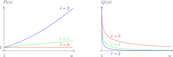
Figure 2: The Legendre functions of first and second kind $P_{l}(u)$ and $Q_{l}(u)$ for $u>1$. We have $P_{l}(1)=1$, whereas $Q_{l}(u)$ diverges for $u\downarrow 1$. Important for the boundary condition of $Z_{l}(u)$ is the different behavior for increasing values of $l$: $P_{l}(u)$ diverges according to (92), whereas $Q_{l}(u)$ converges to zero.

Because the Legendre functions $P_{l}(\sigma)$ do not vanish with increasing $l$, we must require

$$\lim_{l\to\infty}Z_{l}(u)=0\,.$$ (91)

The series of Legendre functions of first kind $P_{l}(u)$ with fixed $u>1$ diverges for $l\to\infty$ according to (grad, , 8.917)

$$P_{0}(u)<P_{1}(u)<P_{2}(u)<\ldots<P_{n}(u)<\ldots\,,\quad u>1\,.$$ (92)

The Legendre functions of second kind $Q_{l}(u)$, however, converge to zero (see Figure 2). Thus, performing the limit $l\to\infty$ in Eq. (90), we obtain

$$1+[Z_{1}(u)-u]Q_{0}(u)=0\,.$$ (93)

From the explicit form arf $Q_{1}(u)=uQ_{0}(u)-1$ it follows that $Z_{1}(u)$ is fixed according to

$$Z_{1}(u)=\frac{Q_{1}(u)}{Q_{0}(u)}\,.$$ (94)

With this we obtain that the result (90) finally reads

$$Z_{l}(u)=\frac{Q_{l}(u)}{Q_{0}(u)}\,,$$ (95)

which is not valid only for $l\not=0$ but also for $l=0$ due to (77).

IV.6 Connection Weight

Inserting (95) into (66) yields the following solution for the connection weight:

$$w(\sigma)=\frac{1}{Q_{0}(u)}\sum_{l=0}^{\infty}(2l+1)Q_{l}(u)P_{l}(\sigma)\,.$$ (96)

Using the identity (grad, , 8.791.1)

$$\sum_{l=0}^{\infty}(2l+1)Q_{l}(u)P_{l}(\sigma)=\frac{1}{u-\sigma}$$ (97)

and (88), we obtain for the connection weight

$$w(\sigma)=\frac{2}{u-\sigma}\left(\ln\frac{u+1}{u-1}\right)^{-1}\,.$$ (98)

Note that integrating (98) over the unit sphere leads to

$$\int\limits_{0}^{2\pi}\!\!d\varphi\int\limits_{-1}^{+1}\!\!d\sigma\,w(\sigma)=4\pi\,,$$ (99)

i.e. the total connection weight coincides with the measure (3).

On the other hand we have to take into account that the self-consistency condition (74) yields an explicit relation between the variable $u$ and the control parameter $\alpha$. Indeed, we infer from (74) and (94) the following transcendental relation between $\alpha$ and $u$

$$\frac{\alpha}{\gamma}=-\frac{2}{3}\left(\ln\frac{u+1}{u-1}\right)^{-1}\left[2\left(\ln\frac{u+1}{u-1}\right)^{-1}-u\right]\,,$$ (100)

which is depicted in Figure 3a.

IV.7 Limiting Cases

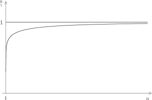
a)       b)

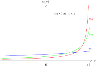
Figure 3: a) Relation (100) between the control parameter $\alpha$ and the variable $u$. b) The connection weight for different values of the control parameter $\alpha$. For decreasing values of $\alpha$ the connection weight around $\sigma=+1$ is growing. In the limiting case $\alpha\to 0$ the connection weight $w(\sigma)$ becomes Dirac’s delta function (107).

The limiting value of (100) for $u\to\infty$ is determined with the help of the expansion (grad, , 1.513)

$$\ln\frac{1+x}{1-x}=2\sum_{k=1}^{\infty}\frac{1}{2k-1}\,x^{2k-1}\,,\quad x^{2}<1\,,$$ (101)

and reads

$$\lim_{u\to\,\infty}\alpha=\gamma\,.$$ (102)

Thus, we conclude that the case $u\to\,\infty$ corresponds to the instability point $\alpha_{c}=f_{1}^{T}f_{1}^{R}$, which was obtained from the linear stability analysis in Section II. Correspondingly, using again (100), we observe that the connection weight (98) coincides in the limit $u\to\infty$ with a uniform distribution:

$$\lim_{\alpha\uparrow\alpha_{c}}w(\sigma)=1\,.$$ (103)

Another biological important special case is $u\downarrow 1$, where we obtain from (100)

$$\lim_{u\downarrow 1}\alpha=0\,.$$ (104)

Furthermore, considering the limit $u\downarrow 1$ in (98) for $\sigma\not=u$, we obtain

$$\lim_{u\downarrow 1}\frac{2}{u-\sigma}\left(\ln\frac{u+1}{u-1}\right)^{-1}=0\,.$$ (105)

On the other hand, integrating (98) for $u\downarrow 1$ over $\sigma$ yields

$$\lim_{u\downarrow 1}\int\limits_{-1}^{1}\frac{2}{u-\sigma}\left(\ln\frac{u+1}{u-1}\right)^{-1}d\sigma=2\,.$$ (106)

Therefore, we conclude that the connection weight $(\ref{117})$ becomes in this limit Dirac’s delta function:

$$\lim_{\alpha\downarrow 0}w(\sigma)=4\delta(\sigma-1)\,.$$ (107)

Thus, decreasing the control parameter $\alpha$ means that the projection between two spheres becomes sharper and sharper (see Figure 3b). A perfect one-to-one retinotopy is achieved for $\alpha=0$ when the uniform and undifferentiated formation of new synapses onto the tectum is completely terminated.

V Summary

In this series of three papers we have analyzed in detail the self-organized formation of retinotopic projections between manifolds of different geometries. Applying our generalized Häussler equations gpw1 to Euclidean manifolds gpw2 , and to spheres in the present paper, led to remarkably analogous results. Both for one-dimensional strings and for spheres we have furnished proof that our generalized Häussler equations describe, indeed, the emergence of a perfect one-to-one retinotopy. Furthermore, we have shown in both cases that the underlying order parameter equations follow from a potential dynamics and do not contain quadratic terms. However, in contrast to strings, spherical manifolds represent a more adequate description for retina and tectum. Therefore, the present paper represents an essential progress in the understanding of the ontogenetic development of neural connections between retina and tectum.

References

- (1) G.J. Goodhill and L.J. Richards, Trends Neurosci. 22, 529 (1999)
- (2) A.F. Häussler and C. von der Malsburg, J. Theoret. Neurobiol. 2, 47 (1983)
- (3) M. Güßmann, A. Pelster, and G. Wunner, Self-Organized Formation of Retinotopic Projections Between Manifolds of Different Geometries – Part 1: The General Model; eprint: physics/0607253
- (4) H. Haken, Synergetics, An Introduction, Third Edition, Springer, Berlin (1983)
- (5) H. Haken, Advanced Synergetics, Springer, Berlin (1983)
- (6) M. Güßmann, A. Pelster, and G. Wunner, Self-Organized Formation of Retinotopic Projections Between Manifolds of Different Geometries – Part 2: Euclidean Manifolds; eprint: physics/0607259
-
(7)
M. Güßmann, Self-Organization between Manifolds of Euclidean and non-Euclidean
Geometry by Cooperation and Competition, Universität Stuttgart, Ph.D. Thesis (2006);
internet: www.itp1.uni-stuttgart.de/publikationen/guessmann_doktor_2006.pdf - (8) H. Kleinert, Path Integrals in Quantum Mechanics, Statistics, Polymer Physics and Financial Markets, 4th ed. World Scientific, Singapore (2006)
- (9) I. S. Gradshteyn and I. M. Ryzhik, Table of Integrals, Series, and Products, 4th ed. Academic Press, New York (1965)
- (10) V. Heine, Group Theory in Quantum Mechanics, Dover, New York (1993)
- (11) W. Wagner and C. von der Malsburg, private communication
- (12) C. Cohen-Tannoudji, B. Diu, and F. Laloë, Quantum Mechanics, Vol. 2, Wiley-Interscience Publication, New York (1977)
- (13) G. B. Arfken and H. J. Weber, Mathematical Methods for Physicists, 5th ed. Academic Press, London (2001)