Helium $2\,^{3}{\rm S}$ - $2\,^{1}{\rm S}$ metrology at $1.557\,\mu{\rm m}$

Abstract

An experiment is proposed to excite the ‘forbidden’ $1s2s\,^{3}{\rm S}_{1}$ - $1s2s\,^{1}{\rm S}_{0}$ magnetic dipole (M1) transition at $1.557\,\mu{\rm m}$ in a collimated and slow atomic beam of metastable helium atoms. It is demonstrated that an excitation rate of $5000\,{\rm s}^{-1}$ can be realised with the beam of a $2\,{\rm W}$ narrowband telecom fiber laser intersecting the atomic beam perpendicularly. A Doppler-limited sub-MHz spectroscopic linewidth is anticipated. Doppler-free excitation of 2% of trapped and cooled atoms may be realised in a one-dimensional optical lattice geometry, using the 2 W laser both for trapping and spectroscopy. The very small (8 Hz) natural linewidth of this transition presents an opportunity for accurate tests of atomic structure calculations of the helium atom. A measurement of the ³He - ⁴He isotope shift allows for accurate determination of the difference in nuclear charge radius of both isotopes.

I Introduction

Measurements of level energies of low-lying states in helium provide very sensitive tests of basic theory of atomic structure. Although helium is a two-electron system, energy levels of the nonrelativistic helium atom can be calculated with a precision that is, for all practical purposes, as good as for nonrelativistic hydrogen. Relativistic corrections to these energies can be calculated in a power series of the fine structure constant $\alpha$ and have been calculated up to $O(\alpha^{2})$. Effects of the finite nuclear mass can be included in a power series of the mass ratio $\mu/M$, where $\mu$ is the reduced electron mass and $M$ the nuclear mass. QED corrections, both hydrogenic and electron-electron terms, up to $O(\alpha^{3})$ have been calculated as well. Effects of the finite nuclear size can be incorporated straightforwardly Drake98 ; Drake04 . Present day theory aims at calculating higher-order corrections (in $\alpha$, $\mu/M$) and cross terms (such as relativistic recoil). The most difficult terms to date are the relativistic and QED terms of $O(\alpha^{4})$ and higher. Higher-order corrections are largest for low-lying S-states and therefore the most sensitive tests of atomic structure calculations can be performed for the $1\,^{1}{\rm S}_{0}$ ground state and the metastable states $2\,^{1}{\rm S}_{0}$ (lifetime 20 ms) and $2\,^{3}{\rm S}_{1}$ (lifetime $8000\,{\rm s}$).

Present-day laser spectroscopy on the low-lying S-states has several disadvantages. To extract an experimental value for the ionisation energy of these states the transition frequency to a high-lying state has to be accurately measured and one has to rely on theoretical values of the ionisation energy of the upper state in the transition. Here the lifetime of the upper state and line shifts due to stray electric fields and laser power are limiting factors. For the ground state, excitation is difficult: one photon of $58\,{\rm nm}$ is required to excite the $2\,^{1}{\rm P}_{1}$ state Eikema97 or two photons of $120\,{\rm nm}$ to excite the $2\,^{1}{\rm S}_{0}$ state Bergeson98 . For the $2\,^{1}{\rm S}_{0}$ and $2\,^{3}{\rm S}_{1}$ metastable states CW laser light is used to excite with one photon the $2\,^{3}{\rm P}$ CancioPastor04 , $3\,^{3}{\rm P}$ Pavone94 ; Mueller05 and ${\rm n}\,^{1}{\rm P}$ Sansonetti92 states. Two-photon spectroscopy is applied to excite the $3\,^{3}{\rm D}$ state Dorrer97 and ${\rm n}\,^{1}{\rm D}$ states Lichten91 .

The most accurate transition frequency measurement to date is for the $2\,^{3}{\rm S}_{1}\rightarrow 2\,^{3}{\rm P}_{0}$ transition CancioPastor04 , with an absolute accuracy of $4\,{\rm kHz}$. This measurement, however, does not provide an accurate measurement of the $2\,^{3}{\rm S}_{1}$ ionisation energy as the $2\,^{3}{\rm P}_{0}$ ionisation energy is not known well enough. Moreover, recent measurements of the fine structure splitting of the $2\,^{3}{\rm P}$ state have shown that experiment and theory do not agree at the $10\,{\rm kHz}$ level Pachucki06a . This very recent finding is considered an outstanding problem of bound state QED and asks for independent measurements on other transitions with similar accuracy. Experimental accuracies for the ionisation energy of the $2\,^{1}{\rm S}_{0}$ and $2\,^{3}{\rm S}_{1}$ states, deduced from measurements to highly excited states and relying on the theoretical calculations of the ionisation energies of these states, are $150\,{\rm kHz}$ and $60\,{\rm kHz}$ respectively. These values agree with but are more accurate than present-day theory for the 2 ¹S₀ and 2 ³S₁ ionisation energy, which is accurate to 5 MHz Morton06a and 1 MHz Pachucki00 respectively. The theoretical accuracies represent the estimated magnitude of uncalculated higher-order terms in QED calculations.

QED shifts largely cancel when identical transitions in different isotopes are studied. Measuring the isotope shift, the main theoretical inaccuracy is in the difference in the rms charge radius of the nuclei Drake05 ; Morton06b . As the charge radius of the ⁴He nucleus is the most accurately known of all nuclei (including the proton) isotope shifts measure the charge radius of the other isotope involved. In this way accurate determination of the 2 ³S₁ - 2 ³P transition isotope shift have allowed accurate measurements of the charge radius of ³He Shiner95 ; Morton06b and the unstable isotope ⁶He Wang04 , challenging nuclear physics calculations. It has to be noted, however, that the measurement of the ⁴He nuclear radius has sofar not been reproduced Morton06b . These measurements therefore primarily measure differences in charge radius.

Elaborating on an idea of Baklanov and Denisov Baklanov97 we propose direct laser excitation of the $2\,^{3}{\rm S}_{1}\rightarrow 2\,^{1}{\rm S}_{0}$ transition in a slow atomic beam or in an optical lattice. This transition has the advantage of an intrinsically narrow natural linewidth of 8 Hz and a wavelength of $1.557\,\mu$m. Also, as the transition connects two states of the same $1s2s$ configuration, the theoretical error in the transition frequency may be smaller than the error in the ionisation energy of the individual states Pachucki06b . The main disadvantage is that the transition is extremely weak; the Einstein A-coefficient for this magnetic dipole (M1) transition is 14 orders of magnitude smaller than for the electric dipole (E1) $2\,^{3}{\rm S}_{1}\rightarrow 2\,^{3}{\rm P}$ transition. In this paper we show that with 2 W of a narrowband fiber laser at $1.557\,\mu$m we can excite more than 1 in $10^{7}$ atoms in an atomic beam experiment or more than 1% of atoms trapped in a one-dimensional standing light wave. Present-day sources of metastable helium atoms Baldwin05 easily provide sufficient atoms in either an atomic beam or in a trap to observe the transition.

II Experimental feasibility

The magnetic dipole transition between the metastable $2\,^{3}{\rm S}_{1}$ state and the $1\,^{1}{\rm S}_{0}$ ground state determines the $\approx 8000\,{\rm s}$ lifetime of the $2\,^{3}{\rm S}_{1}$ state. The experimental and theoretical values of the rate constant for this transition, $1.10(33)\times 10^{-4}$ s^-1 Woodworth75 and $1.272\times 10^{-4}\,{\rm s}^{-1}$ Drake71 ; Lach01 respectively, agree very well. For the electronically similar transition from $2\,^{3}{\rm S}_{1}$ to $2\,^{1}{\rm S}_{0}$, rate constants of $1.5\times 10^{-7}\,{\rm s}^{-1}$ Lin77 and $6.1\times 10^{-8}\,{\rm s}^{-1}$ Baklanov97 have been published. In this letter we will use the value $9.1\times 10^{-8}$ s^-1, obtained by Pachucki Pachucki06b applying the same formalism as used for the calculation of the $2\,^{3}{\rm S}_{1}$ to $1\,^{1}{\rm S}_{0}$ transition rate Lach01 . This value is assumed to be accurate at the 1% level.

In order to evaluate the feasibility of detecting the transition, we need to choose an experimental configuration. Several approaches can be considered Baklanov05 : spectroscopy in a discharge cell, on a thermal or laser-cooled beam, on a cold cloud in a magnetic or optical trap, and ultimately spectroscopy on atoms in an optical lattice. Here, we first consider a relatively simple but promising setup: spectroscopy on a laser-cooled and collimated beam as produced on a daily basis in groups working on BEC in metastable helium Baldwin05 .

III Bloch equations model

In order to describe the excitation of the $2\,^{3}{\rm S}_{1}\rightarrow 2\,^{1}{\rm S}_{0}$ magnetic dipole transition, we use a simplified set of optical Bloch equations (OBE’s).

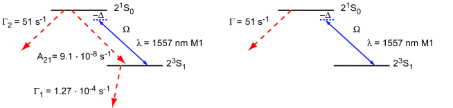
Figure 1: Relevant levels, transitions and decay rates (left) and simplified model (right)

The decay rate of the upper level is fully dominated by the two-photon (2E1) decay to the ground state: $\Gamma_{2}=51\,{\rm s}^{-1}$ Lin77 . Fig. 1 summarizes the relevant decay rates. The driven Rabi frequency of the transition (with atomic frequency $\omega_{21}$) is denoted by $\Omega$, the detuning by $\Delta=\omega_{laser}-\omega_{21}$.

We model this transition by the following set of OBE’s:

$$\dot{\rho_{11}}=A_{21}\rho_{22}-\Gamma_{1}\rho_{11}+i\frac{\Omega}{2}(\rho_{21}-\rho_{12})$$ (1)

$$\dot{\rho_{22}}=-\Gamma_{2}\rho_{22}-i\frac{\Omega}{2}(\rho_{21}-\rho_{12})$$ (2)

$$\dot{\rho_{12}}=-\left(\frac{\Gamma_{1}+\Gamma_{2}}{2}+i\Delta\right)\rho_{12}+i\frac{\Omega}{2}(\rho_{22}-\rho_{11})$$ (3)

$$\dot{\rho_{21}}=-\left(\frac{\Gamma_{1}+\Gamma_{2}}{2}-i\Delta\right)\rho_{21}-i\frac{\Omega}{2}(\rho_{22}-\rho_{11})$$ (4)

As the ground state is not included, this set of equations does not have a steady state state solution except the trivial one ($\rho_{11}=\rho_{22}=\rho_{12}=\rho_{21}=0$).

When we simplify this set of equations by neglecting $A_{21}$ and $\Gamma_{1}$ (which is certainly valid for times $t\ll 1/\Gamma_{1}\approx 8000\,{\rm s}$), it can be solved analytically. Starting at $t=0$ with all atoms in the 2 ${}^{3}{\rm S}_{1}$ state ($\rho_{11}=1$), and denoting $\Gamma_{2}$ by $\Gamma$ from now on, the result for the population $\rho_{22}$ of the 2 ${}^{1}{\rm S}_{0}$ state is:

$$\rho_{22}(t)=\frac{\Omega^{2}}{2\widetilde{\Omega}^{2}}\left[\cosh{\left(\sqrt{\frac{1}{2}[\widetilde{\Omega}^{2}-\widehat{\Omega}^{2}+\frac{\Gamma^{2}}{4}]}\,\,t\right)}-\cos{\left(\sqrt{\frac{1}{2}[\widetilde{\Omega}^{2}+\widehat{\Omega}^{2}-\frac{\Gamma^{2}}{4}]}\,\,t\right)}\right]e^{-\frac{\Gamma}{2}t},$$ (5)

where $\widetilde{\Omega}^{2}\equiv\sqrt{(\Omega+\frac{\Gamma}{2})^{2}+\Delta^{2}}\sqrt{(\Omega-\frac{\Gamma}{2})^{2}+\Delta^{2}}$ and $\widehat{\Omega}^{2}\equiv\Omega^{2}+\Delta^{2}$.

In this Letter, two limiting cases are studied, both valid for short time ($t\ll 2/\Gamma=40$ ms): the weak excitation limit ($1/t\gg\Omega\gg\Gamma/2$) and the strong excitation limit ($\Omega\gg 1/t\gg\Gamma/2$). For the weak excitation limit, Eq. 5 reduces to:

$$\rho_{22}(t)\approx\frac{\Omega^{2}}{\Delta^{2}}\sin^{2}(\Delta\,\,t/2)\equiv\left[\frac{\sin(\Delta\,\,t/2)}{\Delta\,\,t/2}\right]^{2}\frac{\Omega^{2}}{4}t^{2}.$$ (6)

In the strong excitation limit, we can derive a simple expression for the upper level population time-averaged over the oscillations of the cosine in Eq. 5:

$$\langle\rho_{22}\rangle\approx\frac{\Omega^{2}}{2(\Omega^{2}+\Delta^{2})}$$ (7)

IV Broadening effects

Eqs. 6 and 7 allow us to account effectively for both the finite bandwidth of the excitation laser and Doppler broadening effects. For this, we will assume excitation by a purely inhomogeneously broadened light source, i.e., the light is described by a monochromatic field with fixed irradiance $I_{0}$ and a statistical probability distribution $P(\omega)$ for the frequency. The distribution is assumed to be Gaussian, centered at the transition frequency $\omega_{21}$ and with an rms width $\Delta\omega_{rms}\gg 1/\tau$ with $\tau$ the interaction time, i.e., the time at which the upper state population is calculated. The Rabi frequency is given by $\Omega^{2}=\frac{6\pi\,c^{2}}{\hbar\omega_{21}^{3}}A_{21}\langle\,J_{1}\,M_{1}\,1\,-q\,|J_{2}\,M_{2}\rangle^{2}\,I_{0}$ for a $|J_{1},M_{1}\rangle\,\rightarrow|J_{2},M_{2}\rangle$ transition excited by light with polarisation $-q=-1,0,1$. With $J_{1}=1$ and $J_{2}=0$, the non-zero squared Clebsch-Gordan coefficients all equal $\frac{1}{3}$. Assuming the metastable (lower state) atoms to be equally distributed over the three magnetic substates and the polarisation to be pure but arbitrary, the total upper state population can now be evaluated for both the weak and strong excitation limits by integrating Eqs. 6 and 7:

$$\widetilde{\rho_{22}(\tau)}=\frac{\pi^{2}c^{2}}{3\hbar\omega_{21}^{3}}A_{21}\frac{I_{0}}{\sqrt{2\pi}\Delta\omega_{rms}}\tau$$ weak excitation limit (8)

$$\widetilde{\langle\rho_{22}\rangle}=\frac{\pi c}{6}\sqrt{\frac{A_{21}I_{0}}{\hbar\omega_{21}^{3}}}\frac{1}{\Delta\omega_{rms}}$$ strong excitation limit (9)

V Beam experiment

Here we estimate the feasibility of an in-beam spectroscopic experiment on the $1.557\,\mu{\rm m}$ He^∗ $2\,^{3}{\rm S}_{1}\rightarrow 2\,^{1}{\rm S}_{0}$ forbidden transition. The atomic beam is Zeeman-slowed to $100\,{\rm m\,s}^{-1}$ and is transversely cooled to an rms velocity spread of twice the Doppler limit for the He^∗ $2\,^{3}{\rm S}_{1}\rightarrow 2\,^{3}{\rm P}_{2}$ cooling transition ($\Delta v_{rms}=0.6\,\,{\rm ms}^{-1})$. The beam has a diameter of $1\,{\rm cm}$ and an atom flux $\Phi=10^{11}\,{\rm s}^{-1}$. The transition is excited by the beam of a 2 Watt CW fiber laser with a linewidth of $100\,{\rm kHz}$, intersecting the atomic beam perpendicularly. For simplicity, we will assume a flat-top square intensity profile of size $D_{x}\times D_{y}=10\times 10\,{\rm mm}$.

In this experiment, the inverse of the interaction time $1/\tau_{int}=10^{4}\,{\rm s^{-1}}$, the on-resonance Rabi frequency of the transition $\Omega=\sqrt{\frac{2\pi c^{2}}{\hbar\omega_{21}^{3}}A_{21}\frac{P}{D_{x}D_{y}}}=74\,{\rm s}^{-1}$, and half the decay rate $\Gamma/2=25\,{\rm s^{-1}}$. We are sufficiently in the weak excitation limit in this case to allow the use of Eq. 8. The total upper state population now evaluates to $\tilde{\rho}_{22}(\tau)=4.6\times 10^{-7}$. This results in a flux of excited atoms $\Phi_{e}=\tilde{\rho}_{22}(\tau)\Phi=4.6\times 10^{3}\,{\rm s}^{-1}$.

Using $1083\,{\rm nm}$ light resonant with the $2\,^{3}{\rm S}_{1}\rightarrow 2\,^{3}{\rm P}_{2}$ transition, after the interaction region the non-excited fraction of the atoms can be deflected by simple radiation pressure. Using surface ionisation and an electron multiplier on the non-deflected upper state atoms, in principle all excited atoms ($2\,^{1}{\rm S}_{0}$) can then be detected. $2\,^{1}{\rm S}_{0}$ atoms produced by the discharge beam source can be very efficiently suppressed in the laser cooling stages used to prepare the atomic beam. Thus, we can expect a workable signal.

The spectroscopic linewidth of $400\,{\rm kHz}$ is dominated by the Doppler width. Decreasing the Doppler width as well as reducing the laser linewidth are the first steps towards decreasing the spectroscopic linewidth. The limiting homogeneous linewidth is given by the $10\,{\rm kHz}$ interaction time broadening. Applying multiple crossings of laser– and atomic beam using roof-top prisms will not only increase the signal proportionally, but also decrease the interaction time broadening. As a bonus, possible Doppler shifts due to nonorthogonal excitation can be monitored and minimised in this configuration. A schematic view of the proposed setup, with three crossings depicted, is shown in Fig. 2.

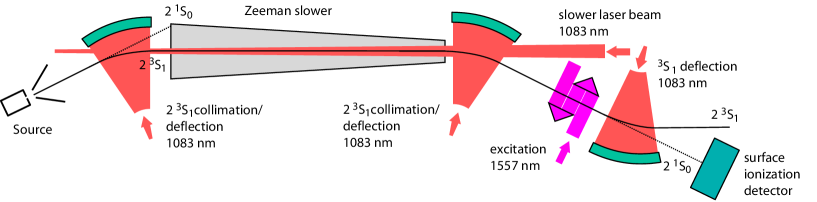
Figure 2: Schematic view of proposed setup.

VI Experiment in an optical lattice

The $1.557\,\mu{\rm m}$ wavelength of the forbidden transition can also serve well to form a far off-resonance optical trap (FORT) for the $2\,^{3}{\rm S}_{1}$ atoms. The dynamic polarisability at this wavelength is fully dominated by the contribution of the $2\,^{3}{\rm S}_{1}\rightarrow 2\,^{3}{\rm P}_{2}$ transition that is resonant at $1.083\,\mu{\rm m}$. This can be used in a next-generation spectroscopy experiment. As the trapping potential is fully insensitive to the wavelength on the scale of a spectroscopic scan of the forbidden transition, a single laser can be simultaneously used for trapping and spectroscopy. We propose using a cold atomic cloud and transferring this cloud to a one-dimensional optical dipole trap formed by a single retroreflected laser beam.

We assume $5\times 10^{7}$ atoms in a cloud with rms size $68\,\mu{\rm m}$ (radial) by $340\,\mu{\rm m}$ (axial) at a temperature of $5\,\mu{\rm K}$, as typically produced along the route to BEC production Tychkov06 . The average density in this cloud then equals $n_{0}=1.0\times 10^{12}\,{\rm cm}^{-3}$. We now assume a more stable 2 Watt fiber laser with a linewidth of $10\,{\rm kHz}$. The trapping/spectroscopy laser beam, directed along the long axis of the cigar-shaped cloud, has a waist radius of $136\,\mu{\rm m}$. This produces a trapping dipole potential with a maximum depth of $24.4\,\mu{\rm K}$, to which the full cloud can be transferred. Analysis of this trap indicates that roughly half the atoms end up in the lowest vibrational state of the standing wave “micro-traps” along the laser beam axis. This will effectively cause a strong Doppler-free part in the spectroscopic signal by Lamb-Dicke narrowing of the transition. The Rabi frequency $\Omega=2\sqrt{\frac{2\pi c^{2}}{\hbar\omega_{21}^{3}}A_{21}\frac{P}{D_{x}D_{y}}}=6.28\times 10^{3}\,{\rm s}^{-1}$, where the extra factor of two is due to the fact that the atoms are now trapped at the antinodes of the standing wave. There is now no a priori fixed interaction time. However, as the Rabi frequency is high we can easily choose the excitation to last a time $t$ satisfying the time-averaged strong excitation limit ($\Omega\gg 1/t\gg\Gamma/2$): $t\gg 0.2$ ms. Eq. 9 then results in an averaged excited state fraction $\widetilde{\langle\rho_{22}\rangle}=\frac{1}{6}\sqrt{\frac{\pi}{2}}\frac{\Omega}{\Delta\omega_{rms}}=2.08\times 10^{-2}$. Given the number of atoms in the trap, every trapped sample will lead to $10^{6}$ atoms in the excited state, which have to be detected. In an experiment, the trapping/excitation laser can be set off-resonance for trapping, and switched to the frequency of the forbidden transition to excite the atoms to the $2\,^{1}{\rm S}_{0}$ state. We can then detect the excited atoms by photoionisation after a few milliseconds of excitation (adjusting the geometry of the ionisation laser beam to ionise all $2\,^{1}{\rm S}_{0}$ atoms expelled from the trap).

An alternative detection option is simply by measuring the increased Penning ionisation that we expect when atoms are excited. The excited $2\,^{1}{\rm S}_{0}$ atoms can also decay through Penning ionisation in collisions with the $2\,^{3}{\rm S}_{1}$ atoms. We assume the rate constant of this process to be $10^{-10}\,{\rm cm}^{3}{\rm s}^{-1}$, i.e., on the order of the rate constant for Penning ionisation of unpolarised atoms in the $2\,^{3}{\rm S}_{1}$ state Stas06 . This results in a decay rate of $\Gamma_{PI}=100\,{\rm s}^{-1}$, leading to a homogeneous broadening of the transition with this value. However, as the dipole shift of the excited $2\,^{1}{\rm S}_{0}$ state has opposite sign, the excited atoms are anti-trapped and escape the cloud of $2\,^{3}{\rm S}_{1}$ atoms in $\tau_{esc}\approx 0.3\,{\rm ms}$. Then Penning ionisation stops, effectively reducing the total $2\,^{1}{\rm S}_{0}$ ionisation rate by a factor of 30 as compared to the case of perfect overlap.

As the Doppler width is effectively eliminated by Lamb-Dicke narrowing, the linewidth is now determined by the laser linewidth. As this width can be further reduced, ultimately the limiting factor will be simply the upper level decay rate.

However, systematic shifts of the transition frequency will have to be carefully considered and corrected for. The largest shift is caused by the difference in dipole shift between the lower and upper level of the transition and amounts to $2.0\,{\rm MHz}$ for the chosen lattice parameters. In optical lattice experiments aiming at optical frequency standards one selects a lattice laser wavelength at which the Stark shift of the lower state equals the Stark shift of the upper state (the ‘magic’ wavelength). For helium there is no practical wavelength available. The highest magic wavelengths are around $410\,{\rm nm}$, where (accidentally) the dipole shift itself is so small that no lattice is feasible at reasonable laser power, and at $351\,{\rm nm}$, where the polarisability is 15 times smaller than at 1.557 $\mu$m and the sign is such that the atoms cannot be confined at antinodes. At 1.557 $\mu$m, combining measurements of the transition frequency at different laser intensities with careful calculations of the intensity-dependent dipole shift will still allow for very accurate extrapolation to zero Stark shift.

Collisional shifts, vanishingly small in the beam experiment, may contribute as well in the lattice experiment. For fermions this shift will be absent at the temperatures considered.

VII Discussion and conclusion

The beam and lattice experiment both promise signal strengths and linewidths that should make a measurement with $1\,{\rm kHz}$ resolution possible. Improvements beyond this level also seem feasible. Standard frequency comb technology easily allows an absolute frequency measurement at this accuracy. A fiber-laser based frequency comb around $1.5\,\mu{\rm m}$ or a titanium-sapphire laser based frequency comb (after frequency doubling) may be used for this purpose.

The main obstacles to be overcome are the residual Doppler linewidth for the beam experiment and the dipole and collisional shifts for the lattice experiment. Another factor to be considered in both experiments is the Zeeman shift due to a stray magnetic field. A solution is to measure only an $\rm{M}=0\rightarrow\rm{M}=0$ transition. For ⁴He, this can be achieved by simply exciting with linearly polarised light. For ³He, it will be important to shield stray magnetic fields and measure both $-\frac{1}{2}\rightarrow-\frac{1}{2}$ and $+\frac{1}{2}\rightarrow+\frac{1}{2}$ transitions and take the average.

What will an absolute frequency measurement at or below the $1\,{\rm kHz}$ level in ⁴He (or ³He) test? In a recent paper Morton, Wu and Drake Morton06a have tabulated the most up-to-date experimental and theoretical ionisation energies, both for ⁴He and ³He. The theoretical uncertainties for the $2\,^{3}{\rm S}_{1}$ and $2\,^{1}{\rm S}_{0}$ states are larger than the experimental error for ⁴He for both states. Experiment and theory agree to well within the error bars. It may be expected that the theoretical error in the 1.557 $\mu$m transition frequency will be smaller than the quadratic sum of the errors in the ionisation energy of the metastable states due to cancellation effects Pachucki06b . Therefore, a measurement of the $2\,^{3}{\rm S}_{1}$ - $2\,^{1}{\rm S}_{0}$ transition frequency will not only provide a direct and accurate link between the ortho (triplet) and para (singlet) helium system but will also test QED calculations more stringently than the existing data.

The isotope shift can be calculated with very high accuracy. Using the most recent values for the nuclear masses and the most recent evaluation of the difference in the square of the nuclear charge radii, i.e., 1.0594(26) fm² Morton06b ; Shiner95 , we deduce a theoretical transition isotope shift of 8034.3712(9) MHz. A measurement of the isotope shift thus provides a very sensitive test of theory. It may also be interpreted as a measurement of the difference in nuclear charge radius of ⁴He and ³He. A measurement at the 1 kHz level will provide this difference with an accuracy of 0.001 fm Drake05 , similar to the accuracy obtained from isotope shift measurements on the $2\,^{3}{\rm S}_{1}$ - $2\,^{3}{\rm P}$ transition. These have been performed with $\sim$5 kHz accuracy Morton06b ; Shiner95 , limited by the 1.6 MHz natural linewidth of that transition. The 8 Hz natural linewidth of the 1.557 $\mu$m transition and the possibilities to improve the beam and lattice experiment further via sub-Doppler cooling resp. uncoupling of the trapping and spectroscopy lasers, may push the accuracy below the 1 kHz level providing new challenges to theorists calculating ionisation energies and, in the case of the isotope shift, provide the most accurate data on differences in nuclear charge radius and nuclear masses of the isotopes involved.

References

- (1) Drake G.W.F. and Martin W.C., Can. J. Phys. 76 (1998) 679.
- (2) Drake G.W.F., Nucl. Phys. A737 (2004) 25.
- (3) Eikema K.S.E., Ubachs W., Vassen W. and Hogervorst W., Phys. Rev. A 55 (1997) 1866.
- (4) Bergeson S.D. et al., Phys. Rev. Lett. 80 (1998) 3475.
- (5) Cancio Pastor P. et al., Phys. Rev. Lett. 92 (2004) 023001.
- (6) Pavone F.S. et al., Phys. Rev. Lett. 73 (1994) 42.
- (7) Mueller P. et al., Phys. Rev. Lett. 94 (2005) 133001.
- (8) Sansonetti C.J. and Gillaspy J.D., Phys. Rev. A 45 (1992) R1.
- (9) Dorrer C. et al., Phys. Rev. Lett. 78 (1997) 3658.
- (10) Lichten W., Shiner D. and Zhou Z-X, Phys. Rev. A 43 (1991) 1663.
- (11) Pachucki K., Phys. Rev. Lett. 97 (2006) 13002.
- (12) Morton D.C., Wu Q. and Drake G.W.F., Can. J. Phys. 84 (2006) 83.
- (13) Pachucki K., Phys. Rev. Lett. 84 (2000) 4561.
- (14) Drake G.W.F., Nörtershäuser W and Yan Z.-C., Can. J. Phys. 83 (2005) 311.
- (15) Morton D.C., Wu Q. and Drake G.W.F., Phys. Rev. A 73 (2006) 034502.
- (16) Shiner D., Dixson R. and Vedantham V., Phys. Rev. Lett. 74 (1995) 3553.
- (17) Wang L.-B. et al., Phys. Rev. Lett. 93 (2004) 142501.
- (18) Baklanov E.V. and Denisov A.V., Quantum Electronics 27 (1997) 463.
- (19) Pachucki K., private communication, 2006.
- (20) Baldwin K., Contemp. Phys. 46 (2005) 105.
- (21) Woodworth J.R. and Moos H.W., Phys. Rev. A 12 (1975) 2455.
- (22) Drake G.W.F., Phys. Rev. A 3 (1971) 908.
- (23) Lach G. and Pachucki K., Phys. Rev. A 64 (2001) 042510.
- (24) Lin C.D., Johnson W.R and Dalgarno A., Phys. Rev. A 15 (1977) 154.
- (25) Baklanov E.V., Pokasov P.V., Primakov D.Yu. and Denisov A.V., Laser Physics 15 (2005) 1068.
- (26) Tychkov A.S. et al., Phys. Rev. A 73 (2006) 031603(R).
- (27) Stas R.J.W., McNamara J.M., Hogervorst W. and Vassen W., Phys. Rev. A 73 (2006) 032713.