Analyzing Trails in Complex Networks

Abstract

Even more interesting than the intricate organization of complex networks are the dynamical behavior of systems which such structures underly. Among the many types of dynamics, one particularly interesting category involves the evolution of trails left by moving agents progressing through random walks and dilating processes in a complex network. The emergence of trails is present in many dynamical process, such as pedestrian traffic, information flow and metabolic pathways. Important problems related with trails include the reconstruction of the trail and the identification of its source, when complete knowledge of the trail is missing. In addition, the following of trails in multi-agent systems represent a particularly interesting situation related to pedestrian dynamics and swarming intelligence. The present work addresses these three issues while taking into account permanent and transient marks left in the visited nodes. Different topologies are considered for trail reconstruction and trail source identification, including four complex networks models and four real networks, namely the Internet, the US airlines network, an email network and the scientific collaboration network of complex network researchers. Our results show that the topology of the network influence in trail reconstruction, source identification and agent dynamics.

‘… when you have eliminated the impossible, whatever remains, however improbable, must be the truth.’ (Sir A. C. Doyle, Sherlock Holmes)

I Introduction

Complex networks have become one of the leading paradigms in science thanks to their ability to represent and model highly intricate structures (e.g., Albert and Barabási (2002); Newman (2003); Boccaletti et al. (2006); da F. Costa et al. (2007)). However, as a growing number of works have shown (e.g., Newman (2003); Boccaletti et al. (2006)) the dynamics of systems whose connectivity is defined by complex networks is often even more complex and interesting than the connectivity of the networks themselves. One particularly interesting type of non-linear dynamics involves the evolution of trails left by moving agents during random walks or dilation processes along the network . The term “dilation” refers to the progressive visiting of neighboring nodes after starting from one or more nodes. For instance, starting from node $i$, at each subsequent time the neighbors of $i$ are visited, then their unvisited neighbor, and so on, defining a hierarchical system of neighborhoods (e.g. Faloutsos et al. (1999); da F. Costa (2004); da Fontoura Costa and Silva (2006)). Although the dynamics is being described as agents visiting network sites, it can be considered also as the evolution on activity in the nodes of the network, where each network edge represents the possibility of activity propagation between the respective nodes. Another important related problem involves attempts to recover incomplete trails. In other words, in cases in which only partial evidence is available to observation, it becomes important to try to infer the full set of visited nodes.

The emergencey of trails has been studied as representing an interesting type of self-organizational system. Helbing et al. Helbing et al. (1997) proposed a model of pedestrian motion in order to explore the evolution of trails in urban green areas. Also, trails have been considered in swarming intelligence analysis Bonabeau et al. (1999); Kennedy and Eberhart (2001) not only as a means to understand animal behavior D.Helbing et al. (1997), but also as a source of insights for new optimization and routing algorithms Dorigo and Gambardella (1997); Dorigo and Stützle (2004). These works considered the evolution of trails in regular grids. However, the communication structures where the trail can be defined are not homogeneous in many cases. Many systems, such as the Internet Faloutsos et al. (1999), social relationships Newman and Park (2003), the distribution of streets in cities Rosvall et al. (2005) and the connections between airports Guimerá and Amaral (2004) are defined by a irregular topology — more specifically, most of these systems are represented by scale-free networks da F. Costa et al. (2007). Here, we study the influence of different topologies in trails recovery, source identification and agent dynamics.

The analysis of trails left in complex networks can have many useful applications. For instance, in information networks the recovery of the trail left by a spreading virus on the Internet can be useful to identify the source of contamination and propose strategies for computer immunization. Similarly, the identification of the origin of rumors, diseases, fads and opinion formation Rodrigues and Costa (2005) are important to understand the human communication dynamics. Another relevant problem is related to traffic improvement and security. In the former case, identification of the covered trails by packages exchanged between computers can help the development of optimal routing paths. In the latter, the source of terrorism strategies and drug trafficking can be determined by analysis of clues identified in social and airline networks. The analysis of trails can also have useful applications in biology. For instance, in ecology, trails analysis can be applied to quantify the interference of human activity in animal behavior and to identify focus of pollution. In paleontology, the recovery of the trails of animal displacement by fossil analysis can help the understanding of diversification between species. In epidemiology, the identification of disease source can help to stop the spreading process as well as to devise effective prevention strategies.

In order to properly represent trails occurring in complex networks, we associate state variables to each node $i$, $i=1,2,\ldots,N$, of the network. The trail is then defined by marking such variables along the respective dynamical process. Only trails generated by self-avoiding random walks and dilations are considered in the current work, which are characterized by the fact that a node is never visited more than once. We restrict our attention to binary trails, characterized by binary state variables . The types of trails can be further classified by considering the marks to be permanent or transient. In the latter case, the mark associated to a node can be deleted after the visit. While many different transient dynamics are possible, we restrict our attention to the following two types: (i) Poissonian, where each mark has a fixed probability of being removed after the visit; and (ii) Evanescent, where the only observable portion of the trail correspond to the node(s) being currently visited.

The current work addresses the problem of recovering trails in complex networks and identifying their origin, while considering permanent and transient binary marks in four different networks models, namely Erdős-Rényi, Watts-Strogatz, Barabási-Albert, and Dorogovtsev-Mendes-Samukhin models; and four real networks: the Internet at the Autonomous System level, the US airlines network, an email network from the University Rovira i Virgili and the scientific collaboration network of complex network researchers. We also consider the analysis of agents propagation considering the four networks models. The next sections start by presenting the basic concepts in complex networks and trails and follow by reporting the simulation results, with respective discussions.

II Basic Concepts in Complex Networks and Trails

An undirected complex network (or graph) $G$ is defined as $G=(V,Q)$, where $V$ is the set of $N$ nodes and $Q$ is the set of $E$ edges of the type $\{i,j\}$, indicating that nodes $i$ and $j$ are bidirectionally connected. Such a network can be completely represented in terms of its adjacency matrix $K$, such that the presence of the edge $\{i,j\}$ is indicated as $K(i,j)=K(j,i)=1$ [otherwise $K(i,j)=K(j,i)=0$]. The degree of a node $i$ corresponds to the number of edges connected to it, which can be calculated as $k(i)=\sum_{j=1}^{N}K(i,j)$. The clustering coefficient is related to the presence of triangles (cycles of length three) in the network Watts and Strogatz (1998). The clustering coefficient of a node $i$ is given by the ratio between the number of edges among the neighbors of $i$ and the maximum possible number of edges among these neighbors; the clustering coefficient of the network is the average of the clustering coefficient of its nodes.

This article considers four theoretical network models and four real complex networks. The network models are (a) Erdős-Rényi — ER Erdős and Rényi (1961), (b) Watts-Strogatz — WS Watts and Strogatz (1998), (c) Barabási-Albert — BA Albert and Barabási (2002) and (d) Dorogovtsev-Mendes-Samukhin — DMS Dorogovtsev et al. (2000). In the first model, networks are constructed by considering constant probability $\lambda$ of connection between any pair of nodes; in the second, networks start with a regular topology, whose nodes are connected in a ring to a defined number $\kappa$ of neighbors in each direction, and later the edges are rewired with a fixed probability; networks of the third and fourth models are grown by starting with $m_{0}$ nodes and progressively adding new nodes with $m$ edges, which are connected to the existing nodes with probability proportional to their degrees (e.g., Albert and Barabási (2002)). The DMS model differs from the BA model by adding an initial attractiveness $k_{0}$ to each node, independent of its degree. When $k_{0}=0$, the DMS model is similar to the BA model Dorogovtsev et al. (2000). All simulations considered in this work assume that the networks have the same number of nodes $N=1000$ and average degree $\left<k\right>=2m=\lambda(N-1)=2\kappa=4$. The real networks considered in this work are the Internet at the level of autonomous systems , the US Airlines Batagelj and Mrvar (2006), the e-mail network from the University Rovira i Virgili (Tarragona) Guimerà et al. (2003) and the scientific collaboration of complex networks researchers .

Trails are generated while subsets of the nodes $V$ are visited during the evolution of random walks or dilations through the network. We assume that just one trail is allowed at any time in a complex network. We consider only self-avoiding random walks, in which no node is visited more than once. At each node, the agent chooses a new node to be visited at random among the not yet visited neighbors of the node. To understand the dilation process, consider $\nu(i)$ the set of neighbors of node $i$. Starting with $i_{o}$, the initial node of the propagation (origin), all nodes in $\nu(i_{0})$ are visited; after that, for all $j\in\nu(i_{0})$, the nodes in $\nu(j)$ not yet visited are recursively visited; this process is repeated for a given number of neighborhood hierarchies (e.g., Faloutsos et al. (1999); da F. Costa (2004); da F. Costa and da Rocha (2006); da Fontoura Costa and Silva (2006)); see Fig. 1.

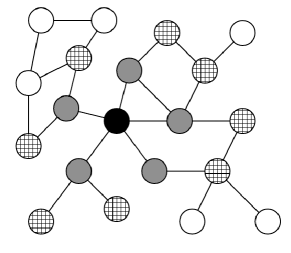
Figure 1: Dilating trail with two levels in a simple network. The origin of this two-hierarchy-trail is the black node, whose immediated neighbors are marked in gray. The nodes with the crossed pattern correspond to the neighbors of the neighbors of the source of the trail. The respective evanescent trail would include only the crossed nodes. A Poissonian version of this trail would imply a ratio $\gamma$ of unmarked (and unobservable) nodes.

In order to represent trails, we associate two binary state variables $v(i)$ and $s(i)$ to each node $i$, which can take the values 0 (not yet visited) or 1 (visited). The state variables $v(i)$ indicate the real visits to each node but are available only to the moving agents, the state variables $s(i)$ are the “marks” of the visits yet available for observation, providing not necessarily complete information about the visits. The structure of the network is assumed to be known to the observer and possibly also to the moving agent(s). Such a situation corresponds to many real problems. For instance, in case the trail is being defined as an exploring agent moves through unknown territory, the agent may keep some visited places marked with physical signs (e.g., flags or stones) which are accessible to observers, while keeping a complete map of visited sites available only to her/himself. Trails are here classified as permanent or transient. In the case of permanent trails, $s(i)=v(i)$, i.e. all visited nodes are known. In the transient type, the state variables $s(i)$ of each node $i$ can be reset to zero after being visited. Transient trails can be further subdivided into: (i) Poissonian, characterized by the fact that each visited node has a fixed probability $\gamma$ of not being observed, i.e. for nodes with $v(i)=1$, $s(i)$ is $1$ with probability $1-\gamma$ and $0$ with probability $\gamma$ (nodes with $v(i)=0$ always have $s(i)=0$); and (ii) Evanescent, where only the last visited nodes are accessible to the observer. Figure 2 shows a classification of the main types of trails considered in this work.

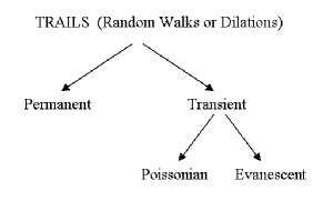
Figure 2: Trails, including those defined by random walks and dilations, can be subdivided as being permanent or transient. The latter type can be further subdivided into Poissonian and Evanescent.

The real extension of a trail is defined as being equal to the sum of the state variables $v(i)$. The observable extension of a trail is equal to the sum of the state variables $s(i)$. Given a trail, we can define the observation error as being equal to

$$\epsilon=\sum_{i=1}^{N}\left[1-\delta(v(i),s(i))\right],$$ (1)

where $\delta(a,b)$ is the Kronecker delta function, yielding one in case $a=b$ and zero otherwise. Note that this error measures the incompleteness of the information provided to the observer. It is also possible to normalize this error by dividing it by $N$, so that $0\leq\epsilon\leq 1$; this normalization is not used in this work.

It is assumed that the observer will try to recover the original, complete, trail from its observation. In this case, the observer applies some heuristic in order to obtain a recovered trail specified by an additional set of state variables $r(i)$ ($r(i)=1$ if node $i$ is in the recovered trail). Such a heuristic may take into account the overlap error between the observable states $s(i)$ and the recovered values $r(i)$, defined as

$$\xi=\sum_{i=1}^{N}\left[1-\delta(s(i),r(i))\right].$$ (2)

Note that as the observer has no access to $v(i)$, the recovery error has to be estimated using $s(i)$. The actual recovery error, which can be used to infer the quality of the recovery, is given by

$$\rho=\sum_{i=1}^{N}\left[1-\delta(v(i),r(i))\right].$$ (3)

Figure 3 illustrates the three state variables related to each network node and the respectively defined errors.

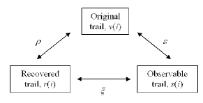
Figure 3: The three state variables associated with each network node $i$ and the defined errors $\epsilon$, $\xi$ and $\rho$.

When using recovery heuristics based on the evaluation of the overlap error, it may happen that two or more different recovered trails yield the same overlap error. In this case, it is interesting to consider two additional parameters in order to quantify the quality of the recovery: (i) the number $M$ of estimated trajectories corresponding to the minimum overlap error; and (ii) the fraction $f$ of times that the correct source can be found among the $M$ recovered trails. When average values of $M$ and $f$ are close to $1$, it means that the recovery strategy is precise.

III Considered Problems

Although the problem of trail analysis in complex networks is potentially very rich and can be extended to many possible interesting situations, for simplicity’s sake we restrict our interest to the three following cases:

Poissonian trails from random walks:

Because the consideration of permanent and evanescent trails left by random walks are trivial , we concentrate our attention on the problem of recovering Poissonian trails left by single moving agents during random walks. Once such a trail is recovered, its source can be estimated as corresponding to one of its two extremities; we do not consider the problem of source identification for this kind of trail. The recovery error is used to measure the quality of the reconstructed trail.

Poissonian trails from dilations:

In this case, only a fraction of the nodes visited by the dilating process is available to the observer. Two problems are of interest here, namely recovering the trail and identifying its origin. To quantify the quality of the recovery, we evaluate the average values of the number of trails with minimal overlap error $\langle M\rangle$ and the fraction of correct source identifications $\langle f\rangle$.

Evanescent trails from dilations:

In this type of problem, only the currently visited nodes are available to the observer, which is requested to reconstruct the trail and infer its possible origin. This corresponds to the potentially most challenging of the considered situations. Note that this case too is subject to random removal of marks, i.e. the values of $s(i)$ are not only of the evanescent type but subjected to be randomly changed to $0$. The results are evaluated by computing $\langle M\rangle$ and $\langle f\rangle$.

IV Strategies for Recovery and Source Identification

Several heuristics can be possibly used for recovering a trail from the information provided by $K$ and $s(i)$. In this work, we consider a strategy based on the topological proximity on the network between nodes with $s(i)=1$ that are not connected. In the case of trails left by random walks, the following algorithm is used:

1. Initialize a list $r$ as being equal to $s$;

2. For each node $i$ with $s(i)=1$:

   1. identify the node $j$ with $r(i)=1$ which is connected to at most one other node with $r(i)=1$ and is closest to $i$ (in the sense of shortest topological path, but excluding shortest paths with length 0 or 1 in the network);

   2. obtain the list $L$ of nodes linking $i$ to $j$ through the respective shortest path (if more than one shortest path exist, one of them is chosen at random);

   3. for each node $k$ in $L$, make $r(k)=1$.

After all nodes with $s(i)=1$ have been considered, the recovered trail will be given by the nodes with $r(i)=1$.

Figure 4 illustrates a simple Poissonian random walk trail, where the black nodes are those in $s$. The original trail is composed of the nodes in $s$ plus the gray nodes. It can be easily verified that the application of the above reconstruction heuristic will properly recover the original trail in this particular case. More specifically, we would have the following sequence of operations:

• node 1 connected to node 5 through the shortest path $(1,2,3,5)$;

• node 2 connected to node 5 (no effect);

• node 5 connected to node 2 (no effect);

• node 9 connected to node 5 through the shortest path $(9,8,6,5)$.

However, if the dashed edge connecting nodes 9 and 10 were included into the network, a large recvery error would have been obtained because the algorithm would link node 9 to node 1 or 2 and not to node 5.

Figure 4: Example of simple Poissonian trail in a network. The black nodes correspond to $s$, the original trail included the black and gray nodes.

A different strategy is used for recovery and source identification in the case of dilation trails, which involves repeating the dilation dynamics while starting from each of the network nodes. The most likely recovered trails are those corresponding to the smallest obtained overlap error. Note that more than one trail may correspond to the smallest error. Also, observe that the possible trail sources are simultaneously determined by this algorithm. Actually, it is an interesting fact that complete recovery of the trail is automatically guaranteed once the original source is properly identified. This is an immediate consequence of the fact that the recovery strategy involves the reproduction of the original dilation, so that the original and obtained trails for the correct source will necessarily be identical.

Some additional remarks are required in order to clarify the reason why more than one trail can be identified as corresponding to the minimal overlap error in Poissonian dilation trails. Figure 5 illustrates a simple network with two trails extending through two hierarchies, one starting from the source A and the other from B, which are respectively identified by the vertical and horizontal patterns. Note that some of the nodes are covered by both trails, being therefore represented by the crossed pattern. Now, assume that the original trail was left by A but that the respectively Poissonian version only incorporated the three nodes with thick border (i.e. all the other nodes along this trail were deleted before presentation to the observer). Because the three nodes are shared by both trails, the same overlap error will be obtained by starting at nodes A or B. It is expected that the higher the value of $\gamma$, the more ambiguous the source identification becomes.

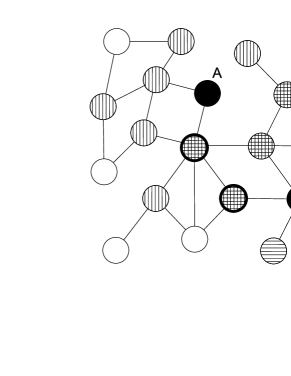
Figure 5: Simple illustration of the source of ambiguity in trail source determination. See text for explanation.

When many possible recovered trails with the same overlap error are found, i.e. when $M>1$, the identification of the source is ambiguous. To take this fact into account, in that cases we consider that each of the possible sources is as good as the other, and therefore can be used as the evaluated source; therefore we make $f=1/M$.

V Simulation Results and Discussion

To evaluate the recovery strategies under different topologies, randomly generated trails are studied in the ER, SW, BA, and DMS network models and the networks of Internet (AS), US Airlines, e-mail and scientific collaboration, as indicated previously. The following sections present e discuss those results.

V.1 Network models

Each considered network model is formed by $N=1\,000$ nodes and average degree $\left<k\right>=4$. All random walk trails were Poissonian with real extent equal to 20 nodes and $\gamma=0.1,0.2,\ldots,0.8$. All dilation trails took place along 2 hierarchies, while the respective Poissonian and evanescent cases assumed $\gamma=0.1,0.2,\ldots,0.8$. In order to provide statistically significant results, each configuration (i.e. type of network, trail and $\gamma$) was simulated 100 times. The rewiring probability in WS model is the same as in ER model, i.e. $p=\left<k\right>/(N-1)$. The initial connectivity in DMS networks models is $k_{0}=5$.

Figure 6 shows the average observation and recovery errors, with respective standard deviations, obtained for the Poissonian random walk trails in the four considered network models. The figure indicates an almost linear increase of the recovery error with $\gamma$. Such a monotonic increase is explained by the fact that the higher the value of $\gamma$, the more incomplete the observable states become. As the recovery of trails with more gaps will necessarily imply more wrongly recovered patches, the respective error therefore will increase with $\gamma$. Also, as can be seen by a comparison between observation and recovery errors, the adopted recovery heuristic allowed moderate results for all considered network models, without significative differences among the models, which suggests that such a recovery strategy is independent of the network topology.

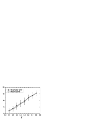
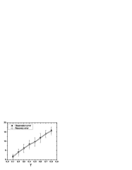
Figure 6: The observation error (black squares) and the recovery errors (white circles) obtained by using the recovery algorithm for for Poissonian trails from random walks in the (a) ER, (b) SW, (c) BA and (d) DMS network models.

Figure 7 gives the average and standard deviation of $M$ for Poissonian dilation trails corresponding to the minimal overlap error $\xi$ for ER, SW, BA and DMS networks. In all of these models, the average and standard deviation values of $M$ tend to increase with $\gamma$, starting at $\left<M\right>=1$. This effect is a consequence of the fact that, the more sparse the information about the real trail, the more likely it is to cover the observable states $s$ with dilations starting from different nodes. Interestingly, the increase of $\left<M\right>$ is substantially more accentuated for ER networks, and BA networks are the least subject to source determination ambiguities.

Figure 7: The average and standard deviations, in terms of $\gamma$, of the number $M$ of detected trails corresponding to the minimal overlap error with respect to Poissonian dilation trails obtained for ER (a), SW (b), BA (c) and DMS (d) network models.

For the Poissonian dilation trails, the average $\left<f\right>$ (and standard deviation) of the flag $f$ is given in terms of $\gamma$ in Figure 8 for ER, SW, BA, and DMS networks. It is clear from these results that the average number of times, along the realizations, in which the correct source is identified among those trails corresponding to the minimal overlap error $\xi$ tends to decrease with $\gamma$. This is a direct consequence of the fact that higher values of $\gamma$ imply substantial distortions to the original trail, ultimately leading to shifts in the identification of the correct source. The behavior of $\left<f\right>$ is similar for ER, BA and DMS network models, with a sharp decrease for $\gamma\gtrsim 0.3$. For SW networks, on the other hand, $\left<f\right>$ has a smooth decrease. The sources of the trails are best identified for ER, BA and DMS when $\gamma\lesssim 0.3$. For higher values of $\gamma$, the sources are best identified for SW network models.

Figure 8: The average (and standard deviations) of the flag $f$ indicating that the correct source has been identified among the detected trails with minimal overlap error $\xi$ in the recovery of Poissonian dilation trails for ER (a), SW (b), BA (c) and DMS (d) network models.

Finally, we turn our attention to transient dilation trails of the evanescent category. Recall that in this type of trails only the current position of the trail (i.e. its border) is available to the observer. Figure 9 presents the average and standard deviation of $M$ obtained, in terms of $\gamma$, for the ER, SW, BA and DMS network models. The result is similar to the case of Poissonian trails (Fig. 7), with the recovery strategy having the worst results for ER networks, and similar results among the other models. But for the evanescent trails $M$ grows more gradually than for Poissonian trails.

Figure 9: The average and standard deviations, in terms of $\gamma$, of the number $M$ of detected evanescent trails corresponding to the minimal overlap error obtained for ER (a), SW (b), BA (c) and DMS (d) network models.

Figure 10 shows the average and standard deviation of the values of the flag $f$ in terms of $\gamma$ obtained for the same models. Again, the results are similar to those obtained for the Poissonian trails (Fig. 8), but with a more gradual decrease of $f$ for the ER model.

Figure 10: The average (and standard deviations) of the flag $f$ indicating that the correct source has been identified among the detected evanescent trails with minimal overlap error $\xi$ for ER (a), SW (b), BA (c) and DMS (d) network models.

Remarkably, though retaining less information about the original trail than the respectively Poissonian counterparts, the evanescent trails tend to allow a similar identification of the source of the trail and the original trail.

V.2 Real networks

We considered four different networks in our simulations, namely: the Internet at the level of autonomous systems, the US Airlines Batagelj and Mrvar (2006), the e-mail network from the University Rovira i Virgili (Tarragona) Guimerà et al. (2003) and the scientific collaboration of complex networks researchers. Table 1 presents some information about these networks. All random walk trails were Poissonian with real extent equal to 20 nodes and all dilation trails took place along 2 hierarchies, with $\gamma=0.1,0.2,\ldots,0.8$. Figure 11 shows average recovery errors, obtained for the Poissonian random walk trails in the four considered real networks. Again, as we observed for the networks models, the recovery error increases almost linearly with $\gamma$, being only slightly smaller than the observation error. The adopted recovery method achieves slightly better results for the US airlines network than for the other networks.

Table 1: Statistical measurements for the considered real networks. $N$ is the number of nodes, $\langle k\rangle$ is the average degree, $cc$ is the average clustering coefficient.

Network	$N$	$\langle k\rangle$	$cc$
Internet	3,522	3.59	0.19
USA Airlines network	332	12.81	0.62
Collaboration in science	1,589	3.45	0.02
E-mail network	1,133	19.24	0.19

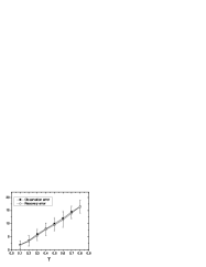
Figure 11: The observation (black squares) and recovery (white circles) errors obtained by using the recovery algorithm for Poissonian trail from random walks, for (a) the Internet, (b) the USA airlines, (c) the e-mail network from the Univeristy Rovira i Virgili, and (d) the scientific collaboration of complex networks researchers.

Figure 12 gives the average and standard deviation of $M$ for trails corresponding to the minimal overlap error $\xi$ for Poissonian dilation trials in the considered real networks. The value of $\left<M\right>$ tends to increase with $\gamma$ for all networks. For the Internet, $\left<M\right>$ has two distinct behavior: (i) for $\gamma\lesssim 0.4$ and $\gamma\gtrsim 0.6$ , $\left<M\right>$ increases slowly, (ii) for $0.4\lesssim\gamma\lesssim 0.6$, $\left<M\right>$ decreases; in the region $\gamma\lesssim 0.5$, $M$ has high standard deviations. In the case of the US Airlines and the scientific collaboration network, $\left<M\right>$ has a similar behavior, but has larger values than from the US Airlines. The smallest values of $\left<M\right>$ are obtained for the e-mail network. Therefore, trails can be better recovery in this type of network, which is an important discovery because it has implications for the identification of the source of spreading of virus or rumors, among other cases.

Figure 12: The average and standard deviations, in terms of $\gamma$, of the number $M$ of detected trails corresponding to the minimal overlap error obtained in the case of Poissonian dilation trails for (a) the Internet, (b) the USA airlines, (c) the e-mail network from the Univeristy Rovira i Virgili, and (d) the scientific collaboration of complex networks researchers.

The average $\left<f\right>$ of the correct source identification flag (and standard deviation) is given in terms of $\gamma$ in Figure 13 for the considered real networks. The source identification is worst for the Internet.

Figure 13: The average (and standard deviations) of the flag $f$ indicating that the correct source has been identified among the detected Poissonian trails with minimal overlap error $\xi$ (a) the Internet, (b) the USA airlines, (c) the e-mail network from the Univeristy Rovira i Virgili, and (d) the scientific collaboration of complex networks researchers.

For transient dilation trails of the evanescent category, the results are shown in Figure 14 (for $M$) and Figure 15 (for $f$). As for the models, the results are close to those obtained considering Poissonian dilation trails, despite the fact that the evanescent category provides less information for trail recovery.

Figure 14: The average and standard deviations, in terms of $\gamma$, of the number $M$ of detected evanescent trails corresponding to the minimal overlap error obtained (a) the Internet, (b) the USA airlines, (c) the e-mail network from the Univeristy Rovira i Virgili, and (d) the scientific collaboration of complex networks researchers.

Figure 15: The average (and standard deviations) of the flag $f$ indicating that the correct source has been identified among the detected evanescent trails with minimal overlap error $\xi$ (a) the Internet, (b) the USA airlines, (c) the e-mail network from the Univeristy Rovira i Virgili, and (d) the scientific collaboration of complex networks researchers.

VI Multi-agents

We considered the dynamics of multi-agents on trail evolution considering four complex networks models: ER, SW, BA and DMS. Each considered network model is formed by $N=1\,000$ nodes and average degree $\left<k\right>=4$. The process is defined as follows: (i) the first agent leaves a gradient trail — the current position has the strongest mark and the source, the weakest — by self avoid random walks, (ii) the path is erased with a probability $\gamma$ (Poissonian trail as before), (iii) the second agent tries to reach the target (the last vertex of the trail) by following preferentially the strongest, at each immediate neighborhood, the marks left by the first agent. When the second agent does not find any mark, it performs a random walk until another mark is found. This process is performed for example by ants in searching of food — the first agent can represent an ant that leaves a trail of pheromone that will be followed by the second ant. The objective of our investigation is to determine the influence of the topology in target identification efficiency, as well as possible overall trajectory minimization, by measuring the length of the path covered by the second agent. All random walk trails were Poissonian with real extent equal to 20 nodes and $\gamma=0.1,0.2,\ldots,0.8$. Figure 16 presents the length of the path covered by the second agent in function of the erasing rate $\gamma$. As can be clearly seen, when $\gamma<0.5$ the second agent covers smallest paths for BA, SW and DMS network models, followed by the ER. This suggests that the topology of the network is fundamental for trajectory following. Indeed, the hubs present in BA and DMS network models provide shortcuts through the network. Enhanced efficiency was also found for the SW network models, but the high clustering coefficient was identified as being fundamental in this case. While the length of the path obtained by the second agent is kept almost constant when $\gamma$ increases for ER, it increases in the remainder models. For $\gamma>0.5$, the length of the path for ER reaches its smallest value. Therefore, when the trail is almost complete, the BA, SW and DMS topologies provide the best performances, but when the trail is sparse, ER allows the shortest paths. Thus, the topology was verified to strongly influence agent dynamics.

Figure 16: The average and standard deviations in terms of the length of the path covered by the second agent obtained for ER (a), SW (b), BA (c) and DMS (d) network models. Each point is an average of 500 realizations.

VII Concluding Remarks

Great part of the interest in complex networks has stemmed from their ability to represent and model intricate natural and human-made structures ranging from the Internet to protein interaction networks. There is a growing interest in the study of dynamics in such systems (e.g., Newman (2003); Boccaletti et al. (2006); Travieso and da F. Costa (2006)). Among the many types of interesting dynamics which can take place on complex networks, we have the evolution of trails left by moving agents during random walks and dilations. In particular, given one of such (possibly incomplete) trails, immediately implied problems involve the recovery of the full trail and the identification of its possible source. Such problems are particularly important because they are directly related to a large number of practical and theoretical situations, including fad and rumor spreading, epidemiology, exploration of new territories, transmission of messages in communications, amongst many other possibilities.

The important problem of analyzing trails left in networks by moving agents during random walks and dilations has been formalized and investigated by using two heuristic algorithms in the present article. We considered four models of complex networks, namely Erdős-Rényi, Barabási-Albert, Watts-Strogatz, and Dorogovtsev-Mendes-Samukhin models, and four different real networks: the Internet at the level of autonomous systems, the US Airlines, the e-mail network from the University Rovira i Virgili (Tarragona) and the scientific collaboration of complex networks researchers. Also, we considered two types of trails: permanent and transient. Particular attention was given to trails with transient marks. In the case of random walk trails, we investigated how incomplete Poissonian trails can be recovered by using a shortest path approach. The recovery and identification of source of dilation trails was approached by reproducing the dilating process for each of the network nodes and comparing the obtained trails with the observable state variables.

It has been shown through simulation that both such strategies are potentially useful for trail reconstruction and source identification. In addition, a series of interesting results and trends have been identified. First, it has been found that the shortest path approach for recovery of trails left by random walks provides similar results for all considered networks and network models, which suggests that such strategy independes on the network topology. Second, for dilatation trails it was found that the Poissonian and evanescent types of trails allow similar efficiency in the identification of sources, despite the fact that the latter trails incorporate less information than the former.

The analysis of multi-agents on networks showed that the topology strongly influences the respective performance. When the trail is almost complete, the Barabási-Albert, Watts-Strogatz and Dorogovtsev-Mendes-Samukhin network models provide the best performance. On the other hand, when the information about the trail is sparse, the final point of the trail is reached faster for the Erdős-Rényi network model.

It is believed that the suggested methods and experimental results have paved the way to a number of important related works, including the investigation of the scaling of the effects and trends identified in the present work to other network sizes, average node degrees and network models. At the same time, it would be interesting to consider graded state variables, more than a single trail taking place simultaneously in a network, other types of random walks (e.g., preferential Travieso and da F. Costa (2006)), as well as alternative recovery and source identification strategies. One particularly promising future possibility regards the recovery of diffusive dynamics in complex networks.

VIII Acknowledgments

Luciano da F. Costa is grateful to CNPq (308231/03-1 and 301303/06-1) and FAPESP (05/00587-5) for financial support. Francisco A. Rodrigues acknowledges FAPESP sponsorship (proc. 04/00492-1).

References

- Albert and Barabási (2002) R. Albert and A.-L. Barabási, Reviews of Modern Physics 74, 48 (2002).
- Newman (2003) M. E. J. Newman, SIAM Review 45, 167 (2003).
- Boccaletti et al. (2006) S. Boccaletti, V. Latora, Y. Moreno, M. Chaves, and D.-U. Hwang, Physics Reports 424, 175 (2006).
- da F. Costa et al. (2007) L. da F. Costa, F. A. Rodrigues, G. Travieso, and P. R. V. Boas, Advances in Physics 56, 167 (2007).
- Faloutsos et al. (1999) M. Faloutsos, P. Faloutsos, and C. Faloutsos, Computer Communication Review 29, 251 (1999).
- da F. Costa (2004) L. da F. Costa, Physical Review Letters 93 (2004).
- da Fontoura Costa and Silva (2006) L. da Fontoura Costa and F. Silva, Journal of Statistical Physics 125, 841 (2006).
- Helbing et al. (1997) D. Helbing, J. Keltsch, and P. Molnár, Nature 388 (1997).
- Bonabeau et al. (1999) E. Bonabeau, M. Dorigo, and G. Theraulaz, Swarm Intelligence: From Natural to Artificial Systems (Oxford University Press, 1999).
- Kennedy and Eberhart (2001) J. Kennedy and R. Eberhart, Swarm Intelligence (Morgan Kaufmann, 2001).
- D.Helbing et al. (1997) D.Helbing, F. Schweitzer, J. Keltsch, and P. Molnár, Physical Review E 56 (1997).
- Dorigo and Gambardella (1997) M. Dorigo and L. Gambardella, BioSystems 43, 73 (1997).
- Dorigo and Stützle (2004) M. Dorigo and T. Stützle, Ant Colony Optimization (MIT Press, 2004).
- Newman and Park (2003) M. E. J. Newman and J. Park, Physical Review E 68 (2003).
- Rosvall et al. (2005) M. Rosvall, A. Trusina, P. Minhagen, and K. Sneppen, Physical Review Letters 94, 028701 (2005).
- Guimerá and Amaral (2004) R. Guimerá and L. Amaral, The European Physical Journal B 38, 381 (2004).
- Rodrigues and Costa (2005) F. A. Rodrigues and L. d. F. Costa, International Journal of Modern Physics C 16 (2005).
- Watts and Strogatz (1998) D. J. Watts and S. H. Strogatz, Nature 393, 440 (1998).
- Erdős and Rényi (1961) P. Erdős and A. Rényi, Acta Mathematica Scientia Hungary 12, 261 (1961).
- Dorogovtsev et al. (2000) S. N. Dorogovtsev, J. F. F. Mendes, and A. N. Samukhin, Phys. Rev. Lett. 85, 4633 (2000).
- Batagelj and Mrvar (2006) V. Batagelj and A. Mrvar, Pajek datasets (2006), http://vlado.fmf.uni-lj.si/pub/networks/data.
- Guimerà et al. (2003) R. Guimerà, L. Danon, A. Díaz-Guilera, F. Giralt, and A. Arenas, Physical Review E 68, 65103 (2003).
- da F. Costa and da Rocha (2006) L. da F. Costa and L. E. C. da Rocha, Eur. Phys. J. B 50 (2006).
- Travieso and da F. Costa (2006) G. Travieso and L. da F. Costa, Physical Review E 74, 036112 (2006).