Selective excitation of metastable atomic states by femto- and attosecond laser pulses

Abstract

The possibility of achieving highly selective excitation of low metastable states of hydrogen and helium atoms by using short laser pulses with reasonable parameters is demonstrated theoretically. Interactions of atoms with the laser field are studied by solving the close-coupling equations without discretization. The parameters of laser pulses are calculated using different kinds of optimization procedures. For the excitation durations of hundreds of femtoseconds direct optimization of the parameters of one and two laser pulses with Gaussian envelopes is used to introduce a number of simple schemes of selective excitation. To treat the case of shorter excitation durations, optimal control theory is used and the calculated optimal fields are approximated by sequences of pulses with reasonable shapes. A new way to achieve selective excitation of metastable atomic states by using sequences of attosecond pulses is introduced.

I Introduction

Nonlinear laser spectroscopy provides new possibilities to create and study selectively excited states of quantum systems Letokhov1977 ; Hansch1977a . Development of the two-photon excitation technique Hansch1977b made it possible to obtain small concentrations of hydrogen in the 2s metastable state. This was sufficient to carry out precise optical measurements of the hyperfine structure of 2s state Kolachevsky2004 and other relativistic and radiative effects Fischer2004 . Metastable atoms and atomic ions also play an important role in excitation and charge transfer processes, even in high-temperature laboratory and astrophysical plasmas JPS1985 . Small concentrations of metastable atoms and atomic ions can significantly affect the radiative spectra of plasmas because of large cross sections of electronic capture to the excited states of highly-charged ions during collisions with the metastable atoms JPS1985 . This conclusion is based on theoretical and indirect spectroscopic observations. Unfortunately, direct measurements are still very difficult due to the low efficiency of modern techniques for the production of beams of metastable atoms Gilbody2003 . The above examples demonstrate the importance of the development of effective methods for selective excitation of metastable atomic states.

Recent progress in laser techniques as well as in theoretical understanding of multiphoton processes in atoms makes it possible to introduce novel methods for effective selective excitation of atomic states by using short laser pulses. A number of approaches to control population transfer between atomic and molecular states have been proposed so far. They can be roughly divided into two groups according to the basic principles. The methods from the first group exploit some known physical mechanisms Allen1987 ; Shore1990 ; Melinger1992 ; Band1997 ; Bergman1998 ; Unanyan2001 ; Gong2004 ; Sola1999 ; Teranishi1997 ; Nagaya2001 ; Zou2005 , e.g., it is possible to introduce some reliable and solvable model equations to estimate the parameters of the controlling laser field analytically, while the methods from the second group are based on the idea of direct variation of the laser field to maximize the desired output Rice2000 ; Shi1988 ; Kosloff1989 ; Ohtsuki1998 ; ZBR1998 .

The schemes from the first group ultimately rely on the properties of $\pi$-pulses or on adiabatic properties. The controlling laser field is found as an accurate or approximate solution of the coupled equations within rotating wave approximation. These schemes, in turn, can be classified by the number of laser pulses involved.

Population inversion achieved by using a single $\pi$-pulse represents the simplest case Allen1987 ; Shore1990 . The frequency of the laser should be in resonance with the transition energy and the control is performed by changing the pulse area. This method can also be used to control multiphoton transitions. In that case, the frequency of the laser pulse should be a fraction of the transition energy so that the energy conservation rules are satisfied. The advantages of this scheme are that it is simple and that the intensity of the controlling laser pulse is relatively small. The main disadvantages are that the efficiency of the scheme is sensitive to the pulse area and that the resonance conditions should be satisfied accurately, especially in the case of multiphoton excitation.

The schemes based on adiabatic rapid passage (ARP) rely on adiabatic properties Allen1987 ; Melinger1992 ; Band1997 . In this case a single chirped laser pulse is used to establish an adiabatic regime so that the complete population transfer occurs as a result of system evolution along the initially populated adiabatic state. The population transfer is not sensitive to the pulse area once an adiabatic regime is established, so the method is quite robust. However, the pulse area must be much larger than in the case of $\pi$-pulses. This becomes critical if the competing ionization or dissociation processes are significant.

Stimulated Raman adiabatic passage (STIRAP) emerged as a very efficient method to provide almost complete population transfer in a three-level system Bergman1998 . In its simplest form, the scheme involves a two-photon Raman process, in which an interaction with a first (pump) pulse links the initial state with an intermediate state, which in turn interacts via a second (Stokes) pulse with a final target state. An important advantage is that almost no population is placed into the intermediate state, and thus the process is insensitive to any possible decay from that state. In more complicated cases the method is used to create a maximal coherent superposition of several states Unanyan2001 and complete population transfer via several intermediate states Gong2004 . The analog of the STIRAP which relies on adiabatic properties is called chirped adiabatic passage by two-photon absorption (CAPTA) Sola1999 .

Recently an effective scheme based on the idea of periodic chirping was introduced Teranishi1997 ; Nagaya2001 . Within this scheme, a sequence of chirped laser pulses or a laser with periodic chirping is used to establish multiple crossings between dressed initial and target levels. Effective laser control is performed by manipulating the parameters of these crossings and adiabatic phase differences between the two crossings directly. In its simplest formulation the complete population transfer can be achieved by using a single quadratically chirped pulse. Because of interference between the crossings, the necessary pulse area of each pulse is much smaller compared to the ARP; however the method is still quite robust. These advantages make the method useful in the field of wave packet control Zou2005 . However, the area of the pulse is still larger than in the case of control by non-chirped pulses.

The methods from the second group are based on maximization of the desired output by a step-by-step adjustment of the controlling field. The main advantage of these methods is that controlling field search is performed explicitly, so that complicated systems can be controlled. These methods can be arranged according to the measure of the controlling parameter space.

In the simplest case, the number of controlling laser pulses and their envelopes are fixed. Each pulse is described by a few parameters: peak intensity, central frequency, chirp rate, central time and full width at half maximum (FWHM). Control is performed by direct optimization of these parameters. By solving the Schrödinger equation, the final population of the desired state can be determined as a function of the parameters of the controlling pulses. Thus, well established numerical procedures for maximization of this function of many variables can be used Press2002 . It is easy to demonstrate that all the schemes discussed above can be reproduced by direct optimization as particular cases. The approach can be considered as an optimization with respect to a finite set of parameters, i.e., in a multi-dimensional space.

To design the controlling field without any restrictions on its shape, the optimal control theory (OCT) was developed Rice2000 ; Shi1988 ; Kosloff1989 ; Ohtsuki1998 ; ZBR1998 . It is based on the idea that the controlling laser pulse should maximize a certain functional. The basic variational procedure leads to a set of equations for the optimal laser field, which include two Schrödinger equations to describe the dynamics starting from the initial and target state wave functions. The optimal laser field is given by the imaginary part of the correlation function of these two wave functions. This system of equations of optimal control must be solved iteratively in general. The reader can find a comprehensive review of OCT in Rice2000 . The main disadvantage of this method is that in many cases the generated optimal field is hardly possible to realize in an experiment. The approach can be considered as optimization with respect to a continious set of parameters, i.e., in the functional space.

In the case of selective excitation of metastable atomic states by laser pulses, a multiphoton interaction is the basic mechanism of the process. Such effects as direct ionization Delone1993 ; DiMauro1995 , resonant transitions via intermediate discrete and continuum states DiMauro1995 ; Freeman1987 ; Kondorskiy2001 ; Kondorskiy2002a ; Kondorskiy2003 , above threshold ionization DiMauro1995 ; Dionissopoulou1995a ; Mercouris1996 ; Dionissopoulou1995b , and electron rescattering by the atomic core Paulus1994 ; Paulus1998 ; Corcum1993 ; Shafer1993 are essential. An accurate treatment of all these effects requires the exact solution of the quantum equations to describe the dynamics of the system. Unfortunately, it is impossible to introduce some reliable and solvable model equations to estimate the parameters of the controlling laser field analytically. Thus, the methods of maximization of desired output should be used.

In the present work selective excitations of the metastable 2s state of hydrogen and the singlet metastable 1s2s ¹S state of helium are studied using both the direct optimization of laser parameters and the optimal control theory. To integrate the time-dependent Schrödinger equation, the well established close-coupling approach based on the properties of time-dependent integral equations Kondorskiy2001 ; Kondorskiy2002a ; Kondorskiy2003 ; Kondorskiy2002b is used. This approach is the most suitable for this kind of spectroscopic calculation. As electron-atom collisions rapidly destroy atomic metastable states, a search of the optimal laser parameters is performed under the requirement that not only high final population of desired metastable state should be achieved, but also ionization probability should be small Kolachevsky2004 ; Fischer2004 .

The present paper is organized as follows. In the next section the theoretical approaches are summarized, and relations between the results of the optimal control calculations and the recently known schemes are demonstrated. In Sec. III direct optimization of the parameters of one- and two laser pulses with Gaussian envelope is used to introduce a number of simple schemes for selective excitation of H(2s) and He(1s2s ¹S). In Sec. IV the optimal control theory is used to look for other possible controlling laser fields. A new mechanism of selective excitation by using attosecond pulses is introduced. Sec. V contains a summary.

II Theory

II.1 Close-coupling approach

The time-dependent Schrödinger equation for an atom in a laser field is written as

$$\left[i\frac{\partial}{\partial t}-\widehat{H}_{0}+\mathbf{F}(t)\mathbf{d}(\mathbf{r})\right]\left|\Psi(t)\right\rangle=0,$$ (1)

where $\widehat{H}_{0}$ is the Hamiltonian of the unperturbed atom, $\mathbf{d}(\mathbf{r})$ is the dipole moment and $\mathbf{F}(t)$ is a laser field. Atomic units are used throughout the paper, unless otherwise noted.

We employ the close-coupling (CC) method on the basis of the orthogonal and normalized unperturbed atomic wave functions of the discrete and continuum states and expand the total wavefunction as

$$\left|\Psi\left(t\right)\right\rangle=\sum\limits_{\nu}a_{\nu}(t)\left|\psi_{\nu}\right\rangle e^{-iE_{\nu}t}$$

$$+\sum\limits_{\mu}\int b_{\mu E}(t)\left|\psi_{\mu E}\right\rangle e^{-iEt}dE$$ (2)

where $\nu$ and $\mu$ are the indices that represent the integer quantum numbers of discrete and continuum states respectively. The functions $\left|\psi_{\nu}\right\rangle$ and $\left|\psi_{\mu E}\right\rangle$ are the corresponding stationary state wavefunctions, $E_{\nu}$ are the energies of the discrete states, $E$ stands for the energy of the electron continuum and $a_{\nu}(t)$ and $b_{\mu E}(t)$ are unknown coefficients.

The Hermitian system of coupled equations for the coefficients of the discrete and continuum states follows from substituting the expansion Eq. (2) into the time-dependent Schrödinger equation Eq. (1) as

$$i\frac{da_{\nu}\left(t\right)}{dt}=\mathbf{F}(t)\sum\limits_{\nu^{\prime}}\mathbf{U}_{\nu\nu^{\prime}}e^{i\left(E_{\nu}-E_{\nu^{\prime}}\right)t}a_{\nu^{\prime}}\left(t\right)$$

$$+\mathbf{F}(t)\sum_{\mu}\int\mathbf{U}_{\nu\mu}(E)e^{i\left(E_{\nu}-E\right)t}b_{\mu E}(t)dE,$$ (3)

$$i\frac{db_{\mu E}\left(t\right)}{dt}=\mathbf{F}(t)\sum\limits_{\nu}\mathbf{U}_{\mu\nu}(E)e^{i\left(E-E_{\nu}\right)t}a_{\nu}\left(t\right)$$

$$+\mathbf{F}(t)\sum_{\mu^{\prime}}\int\mathbf{U}_{\mu\mu^{\prime}}\left(E,E^{\prime}\right)e^{i\left(E-E^{\prime}\right)t}b_{\mu E^{\prime}}(t)dE^{\prime}.$$ (4)

The matrix elements $\mathbf{U}_{\nu\nu^{\prime}}$, $\mathbf{U}_{\nu\mu}(E)$ and $\mathbf{U}_{\mu\mu^{\prime}}(E,E^{\prime})$ are integrals over $\mathbf{r}$-space taken with the atomic dipole moment operator.

The first and the second sums in Eq. (3) describe the bound-bound and free-bound transitions, respectively. These transitions result in a significant redistribution of the population of discrete states. This in turn strongly affects the ionization process Kondorskiy2001 ; Kondorskiy2002a ; Kondorskiy2003 ; Kondorskiy2002b . The first sum in Eq. (4) describes ionization from all the discrete states and the integral term (free-free transitions) describes a multiphoton inverse bremsstrahlung process (within quantum mechanical considerations) or rescattering processes (within quasiclassical considerations). These processes play an important role in formation of the photoelectronic spectra at high energies Paulus1994 ; Paulus1998 ; Corcum1993 ; Shafer1993 . However, since the free-free matrix elements practically do not affect the discrete state amplitudes $a_{\nu}\left(t\right)$, it is possible to neglect them for the evaluation of $a_{\nu}\left(t\right)$. The transitions neglected in this approximation are the third-order (bound-free-free-bound) ones. The role of the free-free transitions was carefully investigated in Refs. Dionissopoulou1995a ; Mercouris1996 ; Dionissopoulou1995b ; Kondorskiy2002a ; Kondorskiy2003 , and this assumption was confirmed to work well.

The close-coupling equations Eqs. (3-4) with the free-free transitions neglected can be solved by discretizing the continuum or by employing the recently developed approach based on the properties of the time-dependent integral equations without any discretization of the continuum Kondorskiy2001 ; Kondorskiy2002a ; Kondorskiy2003 ; Kondorskiy2002b . As the nonresonant interaction between the lower and highly excited discrete states is small, it is possible to adjust the number of discrete states involved in expansion Eq. (2) so that the results of the calculations do not change. Although, strictly speaking, this procedure does not prove the convergence of the close-coupling approach, it is still widely used in collisional physics JPS1985 ; Lebedev1998 .

In the present study we consider excitation and ionization of a single atomic electron in the field of linearly polarized laser pulses.

II.2 Methods of direct optimization of laser parameters

In the simplest case the controlling field is assumed to be a sequence of laser pulses and is written as

$$F(t) = \sum_{j=1}^{N}F_{j}\times f\left(\tau_{j},t-t_{j}\right)$$ (5)

$$\times \sin\left[\omega_{j}\left(t-t_{j}\right)+\alpha_{j}\left(t-t_{j}\right)^{2}\right]$$

where $f\left(\tau,\Delta t\right)$ is a fixed envelope function with FWHM equal to $\tau$ and centered to achieve maximum at time difference $\Delta t=0$. In the present study we focus on the laser pulses Eq. (5) with a Gaussian shape:

$$f\left(\tau,\Delta t\right)=\exp\left[-\frac{4\ln 2}{\tau^{2}}\Delta t^{2}\right].$$ (6)

The system is controlled by changing peak amplitudes $F_{j}$, frequencies $\omega_{j}$, chirp rates $\alpha_{j}$, central times $t_{j}$, and FWHM’s $\tau_{j}$ of the component pulses. By solving the Schrödinger equation one can determine the final population of a selected state as a function of these parameters. To find the maximum of this function, the conjugate gradient search method Press2002 is used here. The gradient of the final population of the target state with respect to the laser parameters is calculated numerically using the finite-difference approximation. The optimization starts from some initial guess parameters.

As different laser pulse parameters have different dimensions, the parameters should be put on a common ground by using dimensionless units, or the optimizations with respect to different types of parameters should be performed separately. In the first case the convergence of the optimization procedure could depend on the dimensionless units used. Indeed, the efficiency of the selective excitation by non-chirped pulse strongly depends on whether or not the resonant conditions are achieved, so that by using common atomic units one should find the maximum of the function that strongly depends on one group of arguments (frequencies) and only weakly on the other arguments (intensities, durations etc.). This example demonstrates that proper dimensionless units should be used to ensure reasonable convergence. Moreover, the derived optimal parameters could depend on how that units are defined.

In the present study the optimizations with respect to different types of parameters are performed separately so that each step of the optimization procedure should contain a set of optimizations with respect to the parameters for all pulses that have the same dimension. Generally, some laser parameters should be linked with each other to achieve a maximum of the desired output. If the chirping rate is zero, the optimal intensity and duration of each pulse are related to each other by some pulse area conservation rule. To avoid this uncertainty, we assume the durations of the pulses to be equal. After the optimal parameters of the controlling sequence of laser pulses are found, we can adjust intensities and durations to fit the specifics of the experimental technique.

The order of optimizations performed at each step of the direct search affects the efficiency, convergence and resulting controlling scheme. However, since the laser field, Eq. (5), has only five different types of parameters, the number of possible nonequivalent orders of optimization is limited. Table 1 presents the correspondence between the controlling schemes generated by the direct optimization method with different orders of optimizations performed at each step and previously known schemes. Since the last schemes have been established without bound-free transitions taken into account the continuum states are not included in the test calculations of Table 1. The continuum states are, however, taken into account at all other calculations, reported in the present paper.

The durations of all the pulses are assumed to be equal and do not change during optimization. Initial parameters used in all the calculations are 1 $GW/cm^{2}$ for intensities of all pulses, frequencies are estimated from the data for the unperturbed atom, chirping rates are zero for all the pulses, centers of the pulses coincide in the cases 1-4 and are equally distant with the $2\cdot$FWHM shift in cases 5 and 6. Our calculations show that number of steps required to achieve convergence is about one and a half the number of laser pulses used in the scheme.

Table 1: Controlling schemes generated by the direct optimization method with different orders of optimizations performed at each step.

Case No.	Number of pulses	Order of optimizations	Known particular cases
1	1	1. Intensities 2. Frequencies	$\pi$-pulses
2	1	1. Intensities 2. Chirping rates	ARP
3	2	1. Central times 2. Intensities 3. Frequencies	Direct excitation or STIRAP
4	2	1. Central times 2. Intensities 3. Chirping rates	Direct excitation or CAPTA
5	Several	1. Frequencies 2. Central times 3. Intensities	Periodic sweeping of laser intensity
6	Several	1. Chirping rates 2. Central times 3. Intensities	Periodic sweeping of laser frequency

The procedure of direct optimization of laser parameters can also be used to calculate intrinsic parameters of the atomic system. For example, by fixing the intensity of the laser and calculating the optimal frequency of selective excitation of different target states, the dynamic Stark shifts of these states can be easily estimated.

II.3 Methods of the optimal control theory

The dynamics of the atom in the laser field is described by the time-dependent Schrödinger equation (1). The initial state wave function $\left|\Phi_{i}(t)\right\rangle$ is specified at time $t=0$. The goal of control is to design such an external field $\mathbf{F}(t)$ that the wave packet calculated with Eq. (1) up to time $t=T$ is close enough to the desired target state wave packet $\left|\Phi_{t}(t)\right\rangle$. One of the most natural and flexible approaches to design such a field is the optimal control theory Rice2000 . It is based on the idea that the controlling laser pulse should maximize a certain functional. The procedure leads to a set of equations for the optimal laser field, which include two Schrödinger equations to describe the dynamics starting from the initial and target state wave packets. The optimal laser field is given by the imaginary part of the correlation function of these two wave packets. This system of equations of optimal control must be solved iteratively in general starting from some initial guess field.

A number of algorithms to realize this idea have been developed Rice2000 ; Shi1988 ; Kosloff1989 ; Ohtsuki1998 ; ZBR1998 . One of the most effective is the algorithm by Zhu, Botina and Rabits ZBR1998 (ZBR algorithm), which is developed to solve the following system of the optimal control equations:

$$\left[i\frac{\partial}{\partial t}-\widehat{H}_{0}+\mathbf{F}(t)\mathbf{d}(\mathbf{r})\right]\left|\phi(t)\right\rangle=0,\quad\left|\phi(0)\right\rangle=\left|\Phi_{i}\right\rangle,$$ (7)

$$\left[i\frac{\partial}{\partial t}-\widehat{H}_{0}+\mathbf{F}(t)\mathbf{d}(\mathbf{r})\right]\left|\chi(t)\right\rangle=0,\quad\left|\chi(T)\right\rangle=\left|\Phi_{t}\right\rangle,$$ (8)

$$\mathbf{F}(t)=-\frac{1}{\gamma}\textrm{Im}\left[\left\langle\phi(t)\right.\left|\chi(t)\right\rangle\left\langle\chi(t)\right|\mathbf{d}(\mathbf{r})\left|\phi(t)\right\rangle\right].$$ (9)

Here $\gamma$ is a positive parameter chosen to weight the significance of the laser energy ZBR1998 . To integrate Eq. (7) forward in time and Eq. (8) backward in time, we employ the close-coupling method discussed in subsection II.1.

To launch the ZBR algorithm, an initial field should be specified. In molecular dynamics control, which is the main area of the application for the ZBR algorithm, a zero initial field is sufficient for most cases. However, since in the present study initial and target states are stationary, a zero initial field cannot be used. Instead we use a single laser pulse of Gaussian shape as an initial field and generate different optimal control fields by changing its parameters. Our calculations show that three to five iterations of the ZBR algorithm are sufficient to achieve the convergence.

III Selective excitation of the metastable atomic states by femtosecond pulses

In the present section selective excitations of H(2s) and He(1s2s ¹S) by one and two femtosecond laser pulses of Gaussian shape are studied. The case of chirp pulses Allen1987 ; Melinger1992 ; Band1997 or periodic chirping Teranishi1997 ; Nagaya2001 is not considered as the pulse area required is larger than in the case of non-chirped pulses. This in turn significantly increases the ionization. However, in some cases when the ionization process is suppressed, periodic chirping can be used to improve the robustness of the scheme. These will be discussed in a future publication.

III.1 Selective excitation of H(2s) and He(1s2s ¹S) by a single laser pulse

In the simplest case a two-photon excitation of H(2s) and He(1s2s ¹S) can be achieved by using a single laser pulse. The process can be affected by changing only three parameters of the laser: frequency, duration, and intensity. To study this case we calculate the final populations of the target metastable states and ionization probabilities as functions of intensity and duration of the laser pulse for two-photon excitation of hydrogen (wavelength is around 240 nm) and helium (wavelength is around 120 nm). The frequency of the laser was optimized for each pair of the arguments to compensate level shifts due to the dynamic Stark effect and to maximize the output.

For the case of selective excitation of H(2s) the maximal values of the target state population achieved are $18~{}\%$ to $20~{}\%$. Unfortunately, the corresponding ionization probabilities are large, $27~{}\%$ to $30~{}\%$. The maximal differences between the target state population and ionization probability are found for the following set of parameters:

$$\text{FWHM [fs]}=2.25\times 10^{14}\text{\Large{/}}I\text{ [W/cm}^{2}\text{]},$$ (10a)

$$\omega\text{ [eV]} =$$ 5.1021 eV (10b)

$$+ 2.34\times 10^{-15}\times I\text{ [W/cm}^{2}\text{]}$$

where $I$ is the pulse intensity. The target state population and ionization probability are found to be $8.4~{}\%$ and $4.2~{}\%$, respectively, for this set of FWHM and $\omega$. Equations (10) are obtained by a fit performed for the range of intensities from 1 TW/cm² to 20 TW/cm².

The efficiency of the process is low because of significance of the one-photon ionization from the target metastable state. As the photon energy is about 5.10 eV to 5.14 eV (depending on pulse intensity), this process populates the continuum states with low energies of about 1.7 eV, so that the corresponding bound-free transition matrix elements are large.

An opposing situation is observed in the case of selective excitation of He(1s2s ¹S). The best values of $65~{}\%$ for the target state population and $26~{}\%$ for ionization probability are found for the following parameters:

$$\text{FWHM [fs]}=7.12\times 10^{15}\text{\Large{/}}I\text{ [W/cm}^{2}\text{]},$$ (11a)

$$\omega\text{ [eV]} =$$ 10.3075 eV (11b)

$$+ 1.54\times 10^{-16}\times I\text{ [W/cm}^{2}\text{]}.$$

Eqations (11) are obtained by a fit performed for the range of intensities from 50 TW/cm² to 400 TW/cm².

The photon energy is about two times higher then in the case of hydrogen (10.3 eV to 10.4 eV, depending on pulse intensity). The process is effective. One-photon ionization from the target metastable state populates the continuum states with energies of about 6.3 eV and corresponding bound-free transition matrix elements are small, so that ionization does not undermine the process.

III.2 Selective excitation of H(2S) by two laser pulses

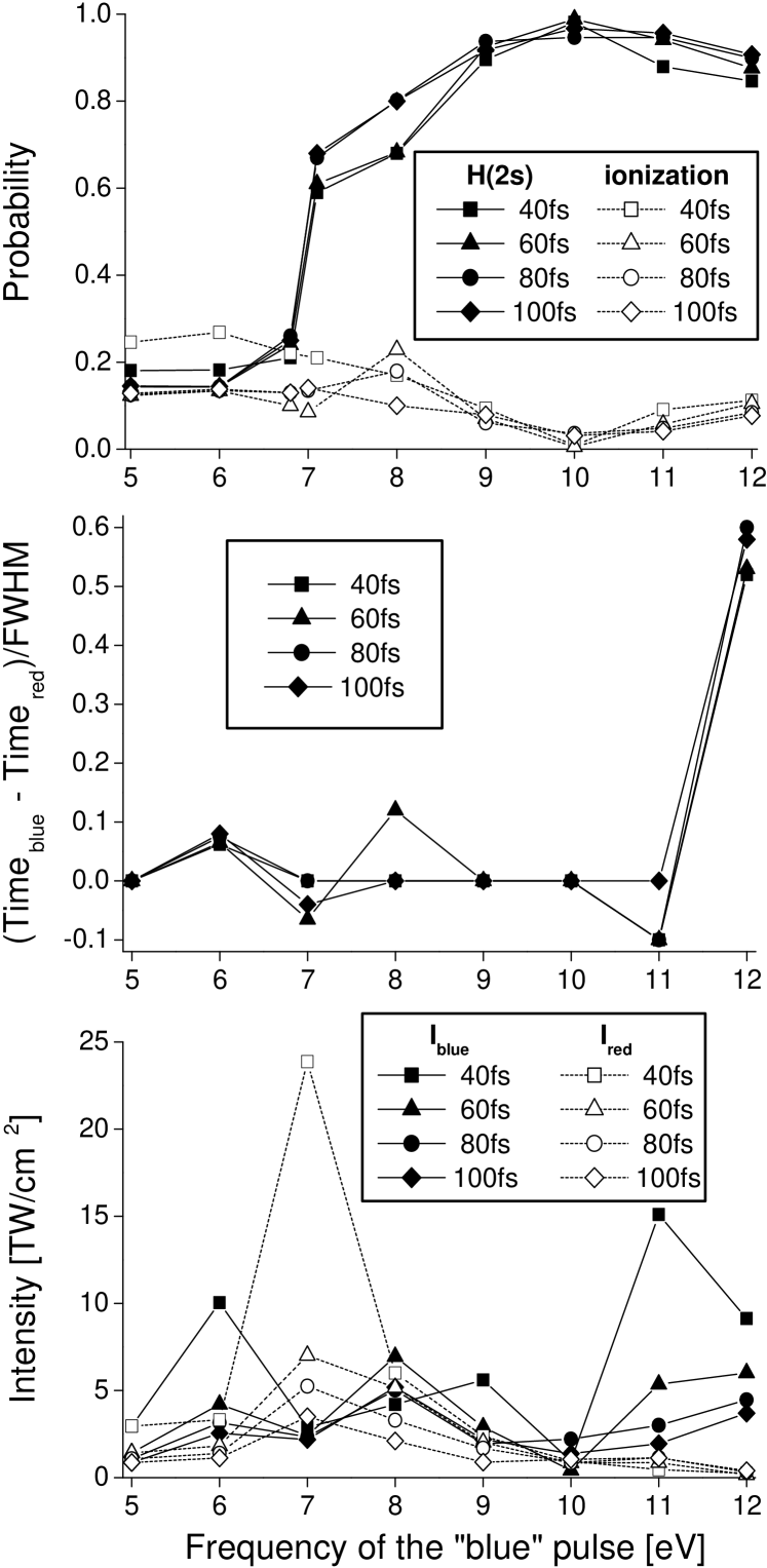
Figure 1: Selective excitation of H(2S) by two laser pulses: (top) final populations of 2s metastable state and ionization probability, (middle) time shift between the “blue” and “red” pulses and (bottom) intensities of the pulses given as functions of frequency of the “blue” pulse.

To improve the efficiency of selective excitation of the metastable state of hydrogen, we increase the number of controlling parameters by introducing two controlling laser pulses with different frequencies instead of a single pulse. For simplicity, we call the pulse with lower frequency as “red” pulse and the pulse with higher frequency as “blue” pulse. Frequencies of the blue and the red pulses should be linked to fit the energy difference between the ground and the metastable states. As optimal intensity and duration of each pulse are approximately related to each other by a pulse envelope area conservation rule, in the present study we fix durations of the pulses to be equal.

Figure 1 presents the final population of the metastable state and ionization probability of hydrogen as functions of frequency of the blue pulse for different durations of the pulses with the frequency of the red pulse, intensities and central times of both pulses adjusted to maximize the population of the metastable state.

If the frequency of the red pulse becomes lower than the threshold of the one-photon ionization of the 2s metastable state, the efficiency of the selective excitation grows dramatically. This is caused by an abrupt decrease of ionization rate, which makes it possible to apply more intense laser pulses and achieve higher selective excitation without increasing the ionization. Unfortunately, for hydrogen the one-photon ionization threshold for the 2s state is equal to one third of the energy difference between the 1s and 2s states, and the simple case, when the blue pulse is produced from the single red pulse by the second harmonic generation, is still not good enough. Acceptable results, however, can be obtained for the frequencies of the blue pulse slightly higher and frequencies of the red pulse slightly lower than the threshold values. An interesting observation comes from the analysis of the time shift between the two optimized controlling pulses. If the frequencies of the pulses are far from being in resonance with some bound state, their centers coincide. However, if the frequency of the blue pulse is close to the frequency of 3p $\rightarrow$ 1s transition, the centers of the blue and the red pulses separate. In this case the direct two-photon excitation process transforms into STIRAP Bergman1998 (Table 1, case 3).

Consider three examples in more detail:

Example 1. Final populations: 2s - 59 %, continuum - 21 %. Parameters of the pulses. Freqencies: blue - 7.12786 eV, red - 3.13629 eV; Intensities: blue - $5.8\times 10^{12}$ $W/cm^{2}$, red - $1.2\times 10^{13}$ $W/cm^{2}$; FWHMs are 40 fs for both pulses; Pulse centers coincide. The frequency of the red pulse is below but close to the threshold of the one-photon ionization of the H(2s) state. Although the frequencies are adjusted to avoid resonances with highly excited discrete states, 7p and 8p states are populated at the level of 9 % and 3 % respectively.

Example 2. Final populations: 2s - 92 %, continuum - 7 %. Parameters of the pulses. Freqencies: blue - 9.09943 eV, red - 1.09933 eV; Intensities: blue - $4.8\times 10^{12}$ $W/cm^{2}$, red - $1.6\times 10^{12}$ $W/cm^{2}$; FWHMs: blue - 40 fs, red - 100 fs; Pulse centers coincide. In this case durations of the pulses are different and efficiency of the process is less sensitive to the shifts between the pulse centers.

Example 3. Final populations: 2s - 91 %, continuum - 8 %. Parameters of the pulses. Freqencies: blue - 12.0878 eV, red - 1.88656 eV; Intensities: blue - $3.7\times 10^{12}$ $W/cm^{2}$, red - $4.0\times 10^{11}$ $W/cm^{2}$; FWHMs are 100 fs for both pulses; blue pulse is delayed for 58 fs. The frequencies of the pulses are close to be in resonance with 3p state. In this case the red pulse comes before the blue pulse. This represents the STIRAP process Bergman1998 .

IV Selective excitation of the metastable atomic states by attosecond pulses

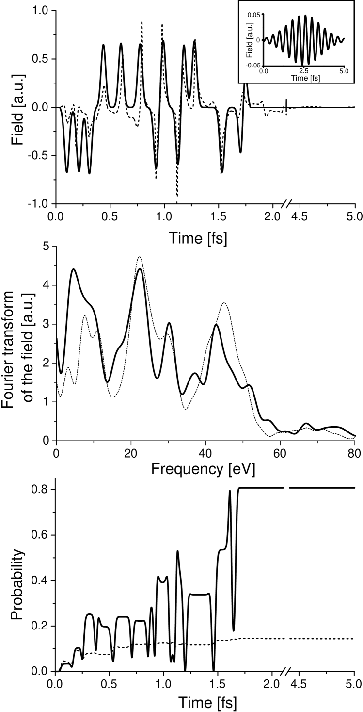
Figure 2: The optimal control field generated for selective excitation of the 1s2s ¹S state of helium (top), its Fourier transform (middle) and time variation of the metastable state population and ionization probability of the controlled atom (bottom). Top and middle: dashed line is the OCT result, solid line is the fitted sequence of attosecond pulses. Insert: initial guess field. Bottom: solid line is the population of the 1s2s ¹S state, dashed line is the ionization probability.

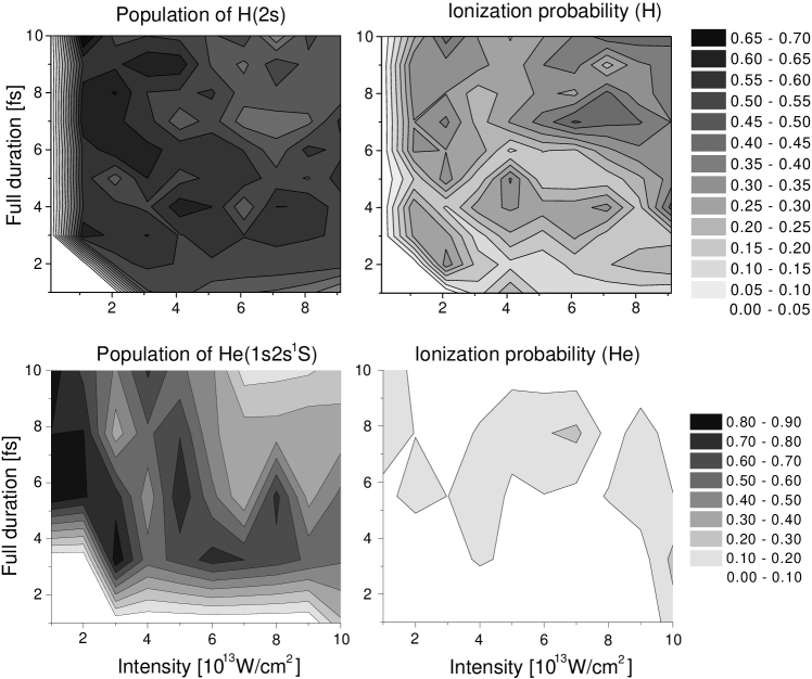
Figure 3: Final populations of the metastable states and ionization probabilities obtained with the optimal field generated from a single Gaussian laser pulse given as a functions of the parameters of initial guess pulse. Top line: Results obtained for selective excitation of H(2s) with the frequency of initial guess pulse is 10.2 eV. Bottom line: Results obtained for selective excitation of H(1s2s ¹S) with the frequency of initial guess pulse is 10.3 eV.

In the previous sections the controlling laser field was assumed to be composed of a few femtosecond laser pulses with Gaussian envelopes. To study other possibilities to achieve selective excitation we use the optimal control theory, as described in Sec. II.3. As the controlling schemes introduced in the previous section for long durations can hardly be improved, we focus on the case of short excitation times.

A typical example is shown in Fig. 2. It presents the optimal control field generated by the ZBR algorithm for selective excitation of 1s2s ¹S state of helium (top) and the time variation of population of the target metastable state and ionization probability during the interaction (bottom). The calculations are performed starting from the Gaussian pulse of intensity 80 TW/cm², frequency 10.3 eV and FWHM 2.5 fs (full duration is 5 fs), which is shown in the insert of Fig. 2. The weight parameter is taken to be $\gamma=0.1$. The final population of the target state is $77~{}\%$ with ionization probability $7~{}\%$. The convergence is achieved in four iterations.

During optimization the laser field completely transforms into a sequence of attosecond pulses. The main perturbations finish after 2 fs, so the duration of active control is also changed. Contrary to the case of controlling femtosecond pulses, the state populations now change abruptly. Physically, the sequence of attosecond laser pulses affects the atomic electrons as a series of pushes. Each push displaces the electrons for a small distance so they can not move far from the atomic core, and this suppresses ionization.

To simplify the optimal control field obtained with the ZBR algorithm we approximate it by a sequence of Gaussians:

$$F(t)=\sum_{j=1}^{N}\frac{A_{j}}{\sqrt{\beta\pi}}\exp\left[-\beta\left(t-t_{j}\right)\right].$$ (12)

If the duration of each pulse is short enough, the momentum supplied to the electrons by each attosecond pulse is given by the pulse area $A_{j}$ and does not depend on $\beta$. To calculate the parameters ${A_{j}}$ and ${t_{j}}$ we roughly approximate the controlling field by sequence (12) and use the method described in Sec. II.2 to optimize ${A_{j}}$ and ${t_{j}}$. The resulting sequence of attosecond pulses is presented in Fig. 2 (top) as a bold line. The calculation is performed with the width parameter $\beta=0.04$ (FWHM = 20 as). The final population of the target state and the ionization probability for that field are $81~{}\%$ and $14~{}\%$, respectively.

Figure 3 presents final populations of the metastable states and ionization probabilities obtained with the optimal fields generated from femtosecond pulses of different intensities and durations. Each point of the plot represents an effective controlling sequence of attosecond pulses. One can see that the results depend on the parameters of the initial guess pulse in a very complicated way. The parameters for some effective controlling sequences of attosecond pulses Eq. (12) calculated by optimal fitting of the parameters ${A_{j}}$ and ${t_{j}}$ are presented in the Table 2.

Recently, q number of schemes to generate trains of attosecond laser pulses have been proposed and realized experimentally (see review Agostini2004 ). The basic idea is the production of a comb of equidistant frequencies in the spectral domain with controlled relative phases. As a result trains of x-ray laser pulses of attosecond duration are obtained. The shapes and carrier frequency can be modified by eliminating certain harmonics. Also, waveforms containing optical bursts approaching one cycle have been successfully synthesized by superposing five phase-controlled sidebands Sokolov2001 . Trains of non-modulated attosecond pulses could be also generated by laser-plasma interaction in the relativistic regime (see Pirozhkov2006 and references therein.)

To generate sequence of pulses close to ones shown in Fig. 2, the spectral components with the frequencies $7.33$ eV, $22.0\approx 3\times 7.3$ eV, $29.3\approx 4\times 7.3$ eV and $44.0\approx 6\times 7.3$ eV should be syncronized. Four main harmonics taken from equidistant spectral modes should be superposed. Thus, for principal frequency of 7.33 eV one should take 1st, 3rd, 4th and 6th harmonics; for principal frequency of 3.66 eV 2nd, 6th, 8th and 12th harmonics, respectively, and so on.

Table 2: Parameters of some effective controlling sequences of attosecond pulses Eq. (12) calculated by optimal fitting of the optimal control fields. Column 1: target atomic state. Colunms 2-4: parameters of the initial guess femtosecond pulse. Columns 5-6: final target state populations and ionization probabilities. Colunms 7-8: Parameters of the sequencies of the attosecond pulses.

Target state	$\omega_{ini}$ $[eV]$	$\text{FWHM}_{ini}$ $[fs]$	$I_{ini}$ $[\text{W/cm}^{2}]$	$P_{target}$	$P_{ion}$	$t_{j}$ $[fs]$	$A_{j}$ $[a.u.]$
H(2s)	10.2	5	$1.0\times 10^{13}$	0.67	0.31	0.05, 0.32, 0.76, 1.33, 1.51, 1.85, 2.02, 2.13, 2.36, 2.41, 2.73	-0.50, -0.44, -0.40, -0.93, -0.44, -0.84, -0.83, -0.93, -0.67, 0.46, 0.95
H(2s)	10.2	3.5	$1.5\times 10^{13}$	0.65	0.29	0.05, 0.69, 1.15, 1.90, 2.27, 2.78, 3.03, 3.23, 3.45, 3.50	0.29, 0.47, 0.30, -0.33, -0.31, -0.44, 0.31, -0.46, 0.61, 0.57
H(2s)	10.2	4.0	$2.3\times 10^{13}$	0.63	0.29	0.05, 0.40, 0.45, 0.77, 0.94, 1.19, 1.34, 1.56, 1.86, 1.93, 2.08, 2.30, 2.45	0.44, 0.41, 0.4, 0.57, 0.41, 0.44, 0.33, 0.26, 0.61, 0.58, 0.49, -0.34, -0.81
H(2s)	10.2	2.0	$7.5\times 10^{13}$	0.62	0.25	0.05, 0.35, 0.68, 1.03, 1.22, 1.30, 1.33, 2.0, 2.45	-0.09, -0.48, -0.34, -0.29, -0.7, -0.23, -0.31, -0.71, -1.43
H(2s)	5.1	5.0	$1.0\times 10^{12}$	0.70	0.20	0.05, 0.25, 0.80, 1.17, 1.50, 1.55, 1.64, 2.14, 2.25, 2.32, 2.70, 2.76	0.24, -0.43, -0.29, -0.43, -0.44, -0.44, -0.29, -0.52, -0.57, -0.59, 0.47, 0.43
H(2s)	5.1	3.5	$1.0\times 10^{12}$	0.67	0.21	0.05, 0.28, 0.55, 0.71, 1.31, 0.96, 1.09	-0.2, 0.13, 0.37, -1.4, -0.57, 0.39, 0.61
H(2s)	5.1	2.5	$1.0\times 10^{12}$	0.65	0.25	0.05, 0.46, 0.87, 1.14, 1.22, 1.42, 1.58, 1.66	0.40, 0.33, 0.19, 0.57, 0.51, 0.52, -0.21, -0.81
He(1s2s 1S)	10.3	5.0	$8.0\times 10^{13}$	0.81	0.14	0.05, 0.16, 0.25, 0.38, 0.54, 0.71, 0.86, 0.92, 1.06, 1.11, 1.21, 1.45, 1.63, 1.65	-0.71, -0.71, -0.73, 0.70, 0.71, 0.71, -0.69, 0.74, -0.69, 0.73, 0.73, -0.71, -0.77, 0.66
He(1s2s 1S)	10.3	5.0	$5.0\times 10^{13}$	0.75	0.10	0.05, 0.11, 0.23, 0.57, 0.73, 0.89, 0.95, 1.07, 1.16, 1.27, 1.32, 1.44, 1.48, 1.64, 1.67	-0.70, -0.66, -0.61, 0.51, -0.54, -0.6, -0.69, 0.86, -0.71, 0.65, -0.76, 0.66, -0.73, -0.71, 0.69
He(1s2s 1S)	10.3	1.0	$2.0\times 10^{14}$	0.78	0.06	0.05, 0.17, 0.24, 0.36, 0.45, 0.51, 0.63, 0.73, 0.76	-0.56, -0.53, -0.89, -0.59, -0.94, 0.81, -0.66, 0.70, -0.79
He(1s2s 1S)	10.3	6	$1.0\times 10^{13}$	0.79	0.10	0.05, 0.25, 0.33, 0.41, 0.57, 0.72, 0.78, 0.90, 0.98, 1.05, 1.15	1.0, 0.88, 0.43, 0.36, 0.51, 0.66, 0.71, 0.74, 0.80, -0.78, 0.90

V Conclusions

In the present study the controlling field search is performed using a well established close-coupling approach for solving the time-dependent Schrödinger equation, so that all essential multiphoton effects are treated accurately. It is demonstrated that optimization procedures provide an effective technique to design laser fields for selective excitation of metastable atomic states. Not only do they reproduce the recently developed schemes of laser control as particular cases but also they introduce new ones.

An efficient selective excitation of H(2s) and He(1s2s ¹S) can be achieved by using one and two femtosecond laser pulses. Frequencies of the pulses should be adjusted properly to suppress single-photon ionization from the target metastable state. Optimal populations of the atomic states and the corresponding parameters of the laser pulses are calculated as functions of preferable frequencies and durations of the pulses. These make it possible to choose the parameters of the controlling laser pulses that fit the capabilities of the present experimental techniques.

A new way to achieve selective excitation of metastable atomic states by using sequences of attosecond pulses is introduced. This is important because of recent progress in production of attosecond pulses. While in the present study the parameters of the pulses are calculated using the optimal control theory, the direct optimization of high harmonics can be used to control the process in the future.

- (1) V. S. Letokhov and V. P. Chebotaev, Nonlinear laser spectroscopy (Springer-Verlag, Berlin-New, York 1977).
- (2) T. W. Hänsch, Nonlinear Spectroscopy, edited by N. Bloembergen (Amsterdam, New-Holland 1977).
- (3) T. W. Hänsch, Laser Spectroscopy III, Springer Series in Optical Sciences 7 edited by J. L. Hall and S. L. Carlsten, (Springer, Berlin-New York 1977).
- (4) N. Kolachevsky, M.Fischer, S. G. Karshenboim and T. W. Hänsch, Phys. Rev. Lett. 92, 033003, (2004).
- (5) M. Fischer et al, Phys. Rev. Lett. 92, 230802, (2004).
- (6) R. K. Janev, L. P. Presnyakov and V. P. Shevelko, Physics of Highly Charged Ions (Springer Verlag, Berlin 1985).
- (7) H. B. Gilbody, private communication (2003).
- (8) L. Allen and J. H. Eberly, Optical Response and Two-Level Atoms (Dover, New York, 1987).
- (9) B. W. Shore, The Theory of Coherent Atomic Excitation (Wiley, New York 1990).
- (10) J. S. Melinger, S. R. Gandhi, A. Hariharan, J. X. Tull and W. S. Warren, Phys. Rev. Lett. 68, 2000 (1992).
- (11) Y. B. Band and P. S. Julienne, J. Chem. Phys. 97, 9107 (1997).
- (12) K. Bergman, H. Theuer and B. W. Shore, Rev. Mod. Phys. 70, 1003 (1998).
- (13) R. G. Unanyan, B. W. Shore and K. Bergmann, Phys. Rev. A 63, 043401 (2001).
- (14) J. Gong and S. A. Rice, Phys. Rev. A 69, 063410 (2004).
- (15) I. R. Solá, V. S. Malinovsky, B. Y. Chang, J. Santamaria and K. Bergmann, Phys. Rev. A. 59, 4494 (1999).
- (16) Y. Teranishi and H. Nakamura, Phys. Rev. Lett. 81, 2032 (1998).
- (17) K. Nagaya Y. Teranishi and H. Nakamura, Advances in Multiphoton Progress and Spectroscopy, edited by R. J. Gordon and Y. Fujimura (World Scientific, Singapore, 2001), Vol. 14.
- (18) S. Zou, A. Kondorskiy, G. Mil’nikov and H. Nakamura, J. Chem. Phys. 122, 084112 (2005).
- (19) S. A. Rice and M. Zhao, Optical Control of Molecular Dynamics (John-Willey & Sons, 2000).
- (20) S. Shi, A. Woody and H. Rabitz, J. Chem. Phys. 88, 6870 (1988).
- (21) R. Kosloff, S. Rice, P. Gaspard, S. Tersigni and D. Tannor, Chem. Phys. 139, 201 (1989).
- (22) Y. Ohtsuki, H. Kono and Y. Fujimura, J. Chem. Phys. 109, 9318 (1998).
- (23) W. Zhu, J. Botina and H. Rabitz, J. Chem. Phys. 108, 1953 (1998).
- (24) W. H. Press, S. A. Teukolsky, W. T. Vetterling and B. P. Flannery, Numerical Recepies in Fortran; Numerical Recepies in C; Numerical Recepies in C++ (Cambridge University Press, 2001-2002).
- (25) N. B. Delone, Basis of Interaction of Laser Radiation with Matter (Gif-Sur-Yvette Cedex-France, Editiones Frontieres 1993).
- (26) L. F. DiMauro and P. Agostini, Adv. At. Mol. Opt. Phys. 35, 79 (1995).
- (27) R.R. Freeman et al, Phys. Rev. Lett., 59, 1092 (1987).
- (28) A. D. Kondorskiy and L. P. Presnyakov, J. Phys. B: At. Mol. Opt. Phys. 34, L663 (2001).
- (29) A. D. Kondorskiy and L. P. Presnyakov, Laser Phys. 12, 449 (2002).
- (30) A. D. Kondorskiy and L. P. Presnyakov, Proc. SPIE 5228, 394 (2003).
- (31) A. Kondorskiy, H. Nakamura, Phys. Rev. A 66, 053412 (2002).
- (32) S. Dionissopoulou, Th. Mercouris, A. Lyras, Y. Komninos and C. A. Nicolaides, Phys. Rev. A 51, 3104 (1995).
- (33) T. Mercouris et al, J. Phys. B: At. Mol. Opt. Phys. 29, L13 (1996).
- (34) S. Dionissopoulou, Th. Mercouris, A. Lyras and C. A. Nicolaides, Phys. Rev. A 55, 4397 (1997).
- (35) G. G. Paulus et al, J. Phys. B: At. Mol. Opt. Phys. 27, L703, (1994).
- (36) G. G. Paulus et al, Phys Rev. Lett. 80, 484 (1998).
- (37) P. Corkum, Phys. Rev. Lett., 71, 1994 (1993).
- (38) K. J. Schafer, Baorui Yang, L. F. DiMauro and K. C. Kulander, Phys. Rev. Lett. 70, 1599 (1993).
- (39) V. S. Lebedev and I. L. Beigman, Physics of Highly Excited Atoms and Ions, (Springer, Berlin-Heidelberg, 1998).
- (40) P. Agostini and L. F. DiMauro, Rep. Prog. Phys., 67, 813 (2004).
- (41) A. V. Sokolov et al, Phys. Rev. A, 63, 051801 (2001); Phys. Rev. Lett, 87, 033402 (2001);
- (42) A. S. Pirozhkov et al, Physics of Plasmas, 13, 013107 (2006).