Knowledge Network Approach to Noise Reduction

Abstract

Previous preliminary results on the application of knowledge networks to noise reduction in stationary harmonic and weakly chaotic signals are extended to more general cases. The formalism gives a novel algorithm from which statistical tests for the identification of deterministic behavior in noisy stationary time series can be constructed.

I Introduction

Noise reduction and identification of underlying deterministic behavior in signals are fundamental questions in fields like communication [16, 13] and time series analysis [7]. A classical model setup relative to the measurement of such signals [16, 13], considers that each observation in a sequence $y_{1},y_{2},...,y_{i},...,y_{T}$ can be decomposed as a sum of a deterministic component and a random perturbation,

$$y_{i}=y(t_{i})=f(t_{i})+\varepsilon(t_{i}).$$ (1)

The random terms $\varepsilon(t_{i})$ are statistically independent from measurement to measurement and independent of $f$. Consider a clean signal that can be adequately modeled by a linear combination of the form

$$f(t_{i})=\sum_{l=1}^{L}a_{l}\varphi(b_{l}t_{i}+c_{l})$$ (2)

where the $\varphi$’s are members of an orthogonal basis of functions. The meaning of adequately modeled in the present context refers to the consistency of $f$ with Eq. (1), in the following sense: if $f$ is approximated through the optimization of some suitable risk or likelihood function in a finite sample, then the residuals should behave like independent random variables. Additionally, if the resulting form of $f$ is expected to be used in a fruitful way for prediction purposes, then $f$ should have the same consistency also outside the original sample, satisfying a suitable goodness criterion as well. In general, the specific nature of the functional basis for $f$ is hidden. For instance, the number of components needed to describe the signal, $L$, is usually unknown beforehand. Previous to any attempt of fitting the data to $f$, the model complexity should be defined. For the setup given by Equations (1) and (2) $L$ gives a quantity that measures the model complexity.

The estimation of $L$ is closely related to the separation of the signal from the noise. In order to see this, consider the case in which $y(t)$ is stationary and $\left<y\right>=0$, where the brackets stand for statistical average. The variance of $y$ is in this case written as

$$\left<y^{2}\right>=\left<\sum_{l_{1}=1}^{L}\sum_{l_{2}=1}^{L}a_{l_{1}}a_{l_{2}}\varphi_{l_{1}}(t_{i})\varphi_{l_{2}}(t_{i})\right>$$ (3)

$$+\left<\varepsilon^{2}\right>.$$

The model complexity $L$ could be estimated from the knowledge of the noise amplitude and some statistical aspects of the components of the basis.

The purpose of the present contribution is to give a novel method for the estimation of the complexity of signal models, which in turn introduces a new framework to deal with noise reduction. The main concern regarding the application of the formalism is on cases in which the noise is strong, that is, with a variance comparable with the corresponding variance of the clean signal. The proposed approach is valuable to the characterization of deterministic signals under strong stochasticity. In many important fields of application, like analysis of geophysical data, voice recognition, time series of economic, ecological or clinic origin, etc., the identification of deterministic behavior is difficult due to the presence of strong additive noise or insufficient sample size. These difficulties are particularily evident for the identification and characterization of low dimensional chaotic behavior in noisy time series. The algorithm introduced here tackle these questions for several important cases. The procedure is linear, yet it is able to perform signal analysis tasks that are beyond the capabilities of traditional linear noise reduction techniques.

I-A Knowledge Networks

The proposed method relies on the notion of a knowledge network [8, 1]. Knowledge networks have been originally motivated from the study of some particular structures that arise in economy and biology, like interactions between consumers and products in a market or protein – substrate interactions [8, 9]. A knowledge network is defined as a network in which the nodes are characterized by $L$ internal degrees of freedom, while their edges carry scalar products of vectors on two nodes they connect [8]. In order to fix ideas, consider the following knowledge network model of opinion formation [8, 1]: suppose that there exists a database of opinions given by agents on a given set of products. This database can be seen as a sparse matrix, with holes corresponding to missing opinions (say, agents that have never been exposed to a given product). In geometrical words, the preferences of an agent are represented as a vector in an hypothetical taste space, whose dimension and base vectors are generally unknown. A product is represented by a similar vector of qualities. An agent’s opinion on a given product is assumed to be proportional to the overlap between preferences and qualities, which can be expressed by the scalar product between corresponding vectors. Therefore, products act like a basis, and opinions as agent’s coordinates on such a basis. Consider a population of $M$ agents interacting with $N$ products. The two sets of vectors lie in a $L$-dimensional space, ${\bf a}_{n}=(a^{1},a^{2},...,a^{L})$ and ${\bf b}_{m}=(b^{1},b^{2},...,b^{L})$, where $n=1,2,...,N$ and $m=1,2,...,M$. In this way the overlap $y_{m,n}={\bf b}_{m}\cdot{\bf a}_{n}$ represents the opinion of agent ${\bf b}_{m}$ on product ${\bf a}_{n}$. Only the overlaps $y_{m,n}={\bf b}_{m}\cdot{\bf a}_{n}$ can be directly observable. The issue is then to reconstruct the hidden quantities from a known fraction of the scalar products. For the case in which $L$ is known, Maslov and Zhang [8] have shown the existence of thresholds for the fraction $p$ of known overlaps, above which is possible to reconstruct at different extents the missing information. Bagnoli, Berrones and Franci [1], have generalized the study of Maslov and Zhang to the case in which the dimensionality $L$ is unknown. The present work mainly relies on this last approach, so a brief summary of the results of Bagnoli, Berrones and Franci is now presented.

Suposse that the components of $\bf{b}_{m}$ and $\bf{a}_{n}$ are random variables distributed according to

$$P(a_{n}^{l},b_{m}^{l})=P_{n,l}(a)P_{m,l}(b),$$ (4)

and define $\left<h\right>$ as the average, computed in the thermodynamic limit, over $P(a_{n}^{l},b_{m}^{l})$ of an arbitrary function $h(a_{n}^{l},b_{m}^{l})$. For a set of hidden components distributed according to Eq. (4), the $y$’s are uncorrelated in the thermodynamic limit. However, correlations arise because $L$ is finite.

In order to kept the expressions simple, it is assumed that $\left<a_{n}^{l}\right>=\left<b_{n}^{l}\right>=0$. Averaging over the distribution (4) the variance of the overlaps is written as

$$\left<y^{2}\right>=L\left<a^{2}\right>\left<b^{2}\right>.$$ (5)

For this model setup, Bagnoli, Berrones and Franci [1] have shown that any overlap can be expressed in terms of a weighted average of other overlaps,

$$y_{m,n}=\frac{L}{M-1}\sum_{i=1}^{M}C_{m,i}y_{i,n}+\epsilon_{L,M,N},\quad i\neq m,$$ (6)

where $C_{i,j}$ is the correlation among $y_{i}$ and $y_{j}$, specifically, the correlation calculated over the expressed opinions of agents $i$ and $j$ on different products. This correlation asymptotically goes to the overlap between the corresponding vectors of agents tastes. The hidden quantity $L$ can be extracted by fitting the proportionality factor $\frac{L}{M-1}$.

The error term $\epsilon$ is at first order given by

$$\epsilon\sim\sqrt{\left<a^{2}\right>\left<b^{2}\right>}L^{3/2}\frac{\sqrt{M}+\sqrt{N}}{\sqrt{MN}},$$ (7)

An aspect of this formalism that is important for applications is that there is no necessity to have a fully connected opinion matrix. The results are extended to sparse datasets simply by the redefinition of the parameters $M$ and $N$ like functions of the pair $(m,n)$. In this way $M_{n}$ represents the available number of opinions over product $n$ given by any agent and $N_{m}$ is the number of opinions expressed by agent $m$ regarding any product [1].

I-B Knowledge Networks and Signal Models

As already pointed out in [3], a knowledge network framework for signals as those described by Eqs. (1) and (2) can be built for certain classes of stationary signals. The essential point is the assumption that a distribution for the components of the signal model exists, analogous to distribution (4). If $N$ time ordered subsamples of size $M$ are extracted from the observed sequence $y_{1},y_{2},...,y_{i},...,y_{T}$, we refer to $y_{m,n}$ as the measured value at time $m$ in subsample $n$, with $n=1,2,...,N$ and $m=1,2,...,M$. The distribution of the components of $y_{m,n}$ is assumed to be

$$P(a_{n,l},\varphi_{m,n,l})=P_{n,l}(a)P_{m,n,l}(\varphi).$$ (8)

In order to see how a distribution $P(a_{n,l},\varphi_{m,n,l})$ can arise for the problem in hands, note that from Equations (1) and (2) follows that

$$y_{m,n}=\sum_{l=1}^{L}a_{n,l}\varphi(mb_{n,l}+c_{n,l})+\varepsilon_{m,n}.$$ (9)

For fixed $L$, the parameters $a_{n,l}$, $b_{n,l}$ and $c_{n,l}$ are chosen to be optimal in the given sample with respect to some suitable risk or likelihood function [4]. Due to the noise and to the finite sample size, the chosen parameters fluctuate from sample to sample, giving rise to a distribution of the form $P(a_{n,l},\varphi_{m,n,l})$.

In the next Section a formalism for noise reduction in signals is built under the assumption (8). The close connection between the problem of noise reduction and estimation of model complexity is shown, leading to a new technique for model complexity estimation in stationary signals. In Section III the resulting algorithm is numerically tested on several examples, that are relevant to important potential applications. Final remarks and a brief discussion of future work is given in Section IV.

II Noise Reduction by Knowledge Networks

Consider the following linear transformation of the components

$$a_{n,l}\to a_{n,l}-\left<a_{l}\right>$$ (10)

$$\varphi_{m,n,l}\to\varphi_{m,n,l}-\left<\varphi_{m,l}\right>,$$

where

$$\left<a_{l}\right>=\sum_{n}a_{n,l}P_{n,l}(a)$$ (11)

$$\left<\varphi_{m,l}\right>=\sum_{n}\varphi_{m,n,l}P_{m,n,l}(\varphi)$$

Introducing the definitions

$$A=\left(\begin{array}[]{c c c}a_{1,1}&...&a_{N,1}\\ .&&.\\ .&&.\\ .&&.\\ a_{1,L}&...&a_{N,L}\end{array}\right),\Phi_{n}=\left(\begin{array}[]{c c c }\varphi_{1,1,n}&...&\varphi_{M,1,n}\\ .&&.\\ .&&.\\ .&&.\\ \varphi_{1,L,n}&...&\varphi_{M,L,n}\\ \end{array}\right)$$ (22)

and

$$\Gamma=\left(\begin{array}[]{c c c}\varepsilon_{1,1}&...&\varepsilon_{1,N}\\ .&&.\\ .&&.\\ .&&.\\ \varepsilon_{M,1}&...&\varepsilon_{M,N}\end{array}\right),$$ (28)

the model setup given by Eq. (9) can be written in matricial form as

$$Y=\Phi_{n}^{\tau}A+\Gamma.$$ (29)

In the limit $N\to\infty$ the operation $AA^{\tau}$ goes to

$$AA^{\tau}=N\left(\begin{array}[]{c c c c }\left<a_{1}^{2}\right>&0&...&0\\ 0&\left<a_{2}^{2}\right>&...&0\\ .&.&&.\\ .&.&&.\\ .&.&&.\\ 0&0&...&\left<a_{L}^{2}\right>\end{array}\right).$$ (36)

In the same way, in the limit $M\to\infty$

$$\Phi\Phi^{\tau}=M\left(\begin{array}[]{c c c c }\left<\varphi_{1}^{2}\right>&0&...&0\\ 0&\left<\varphi_{2}^{2}\right>&...&0\\ .&.&&.\\ .&.&&.\\ .&.&&.\\ 0&0&...&\left<\varphi_{L}^{2}\right>\end{array}\right).$$ (43)

The form of the diagonal elments in Ec. (43) follows from an additional ergodicity assumption: the average $\left<\varphi_{l}^{2}\right>$ can be equivalently taken over infinitely many finite samples or over a single sample of infinite length. For stationary signals the validity of this assumption is straightforward.

Consider the operation

$$\hat{Y}=\frac{k}{M}CY,$$ (44)

where $C$ is the correlation matrix of the $y$’s. It is now shown that if $\left<a_{l}^{2}\right>=\left<a^{2}\right>$ and $\left<\varphi_{l}^{2}\right>=\left<\varphi^{2}\right>$, that is, if the variabilty due to finite sample size, discrete sampling and noise affect in the same way all of the components, then $\hat{Y}=Y-\Gamma$ in the limit $N\to\infty$, $M\to\infty$, using a suitable value for the factor $k$. The formula (44) is expanded as

$$\hat{Y}=\frac{k}{M}\frac{YY^{\tau}}{\left<y^{2}\right>}Y =$$ (45)

$$\frac{k}{M}\frac{\left[\Phi^{\tau}A+\Gamma\right]\left[A^{\tau}\Phi+\Gamma^{\tau}\right]}{N\left[L\right<a^{2}\left>\right<\varphi^{2}\left>+\right<\varepsilon^{2}\left>\right]}Y =$$

$$\frac{k}{M}\frac{\left[\Phi^{\tau}AA^{\tau}\Phi\Phi^{\tau}A+\Gamma\Gamma^{\tau}\Phi^{\tau}A\right]}{N\left[L\right<a^{2}\left>\right<\varphi^{2}\left>+\right<\varepsilon^{2}\left>\right]}.$$

Introducing the results (36) and (43) into Eq. (45)

$$\hat{Y}=\frac{k}{M}\frac{M\left<a^{2}\right>\left<\varphi^{2}\right>+\left<\varepsilon^{2}\right>}{L\left<a^{2}\right>\left<\varphi^{2}\right>+\left<\varepsilon^{2}\right>}\Phi^{\tau}A.$$ (46)

The factor $k$ must therefore be chosen as

$$k=\frac{M[L\left<a^{2}\right>\left<\varphi^{2}\right>+\left<\varepsilon^{2}\right>]}{M\left<a^{2}\right>\left<\varphi^{2}\right>+\left<\varepsilon^{2}\right>}$$ (47)

The fluctuations of the observable $y(t)$ can be decomposed as

$$\left<y^{2}\right>=L\left<a^{2}\right>\left<\varphi^{2}\right>+\left<\varepsilon^{2}\right>.$$ (48)

Introducing Eq. (48) into Eq. (47), an expression for $L$ in terms of measurable quantities is found

$$L=\frac{\alpha M[\left<y^{2}\right>-\left<\varepsilon^{2}\right>]}{\left<y^{2}\right>-\alpha\left<\varepsilon^{2}\right>},$$ (49)

where $\alpha=\frac{k}{M}$. In order to see how the terms appearing at the right in Eq. (49) are measured, consider the following algorithm for noise reduction and estimation of the optimum complexity in models for stationary signals. The anticipation formula in this case reads

$$\hat{y}(t_{i})=\frac{k}{M}\sum_{h=1,h\neq i}^{M}C(t_{h})y(t_{i}-t_{h}).$$ (50)

The signal is processed performing the following steps:

i) Calculate the autocorrelation function $C(t)$.

ii) Perform mean squares over a sample of $M$ consecutive points to estimate the factor $\alpha=\frac{k}{M}$ in Eq. (50).

The mean squares problem can be solved exactly, giving

$$\alpha=\frac{\sum_{i=1}^{M}y(t_{i})\sum_{\tau=1}^{M}C(t_{\tau})y(t_{i}-t_{\tau})}{\sum_{j=1}^{M}\sum_{\tau_{1}=1}^{M}C(t_{\tau_{1}})y(t_{j}-t_{\tau_{1}})\sum_{\tau_{2}=1}^{M}C(t_{\tau_{2}})y(t_{j}-t_{\tau_{2}})}$$ (51)

$$i\neq\tau,j\neq\tau_{1},j\neq\tau_{2},$$

with $M$ less than or equal to one half of the total lenght of the signal. The term $\left<\varepsilon^{2}\right>$ is estimated after the filtering, using the filtered data as an approximation of the underlying deterministic signal and performing the substraction $\left<\varepsilon^{2}\right>=\left<y^{2}\right>-\left<f^{2}\right>$

iii) By the use of Eq. (49), calculate $L$ in terms of observable quantities.

The steps i) – iii) define what hereafter is called the Knowledge Network Noise Reduction (KNNR) algorithm.

III Examples

The KNNR algorithm is tested on data generated numerically, adding at each time step a Gaussian white noise term $\varepsilon(t)$ to a deterministic function $f(t)$. The simulation of the noise is based on the L’Ecuyer algorithm, which is known to accomplish adecuate performance with respect to the main statistical tests, and to produce sequences of random numbers with lenght $\sim 10^{18}$ [11]. The noisy data $y(t)=f(t)+\varepsilon(t)$ enters as input for the KNNR algorithm. By the use of the Fast Fourier Transform of the input [11], the autocorrelation function is calculated for a maximum lag equal to one half of the total length of the signal. The steps ii) and iii) of the KNNR algorithm are then performed over the second half of the input.

The capabilities for noise reduction in harmonic and weakly chaotic time series of the proposed method have already been discussed in [3].

The KNNR framework provides a characterization of the signal model complexity in terms of $L$, the number of member functions of a certain orthogonal basis needed to describe the signal, if it is indeed separable into a deterministic component and a white noise term. If the necessary assumptions are met, $L$ should converge to a finite value as the sample size grows. This fact can be used to identify underliyng deterministic behavior.

In the next examples the KNNR approach is tested on several chaotic systems, with and without additive noise, and for camparision purposes, on purely stochastic systems as well. The mean value of the signals is substracted before they enter as input in the KNNR algorithm. The examples with a deterministic part are therefore constructed by

$$y_{i}=s_{i}+\varepsilon_{i}-\left<y\right>,$$ (52)

where $y_{i}$ is the input and $s_{i}$ is given by the iteration of a nonlinear discrete map. Each of the noise terms $\varepsilon_{i}$, is independently drawn from a Gaussian distribution.

The KNNR algorithm is capable to perform tasks that are beyond the scope of traditional linear signal processing techniques. For instance, with large enough sample size, the KNNR algorithm is able to identify nonlinear behavior in signals whose power spectrum is consistent with a correlated stochastic process. This identification is not possible by classical approaches like the Wiener filter [16], which relies in a clear separation between oscillatory and noise components in the spectrum. More recent methods, like surrogate data [15] or nonlinear techiques [2], on the other hand, do not give a comprehensive framework to deal with noise reduction and identification of determinism in a common ground.

III-A The Logistic Map

An archetypal example of a simple nonlinear system capable of chaotic behavior is given by the logistic map [10]

$$s_{i}=rs_{i-1}(1-s_{i-1}).$$ (53)

With a parameter value of $r=3.6$ and initial conditions in the interval $(0,1)$, the map (53) displays a weakly chaotic behavior, close to quasi – periodic motion. As already discussed in [3], in this case $L\sim 2$, indicating that with this low model complexity is possible to accomplish the separation dictated by Eqs. (1) and (2).

A case with $r=3.7$ and the initial condition in the interval $(0,1)$ is analyzed with the KNNR algorithm. The map is perturbed by a Gaussian white noise with a variance of $0.2$, essentially the same variance of the clean signal.

The power spectrum taken from a sample of $16384$ points of the input signal is presented in Fig. 1. Besides the presence of some relevant peaks at high frequencies, the spectrum is basically a white noise.

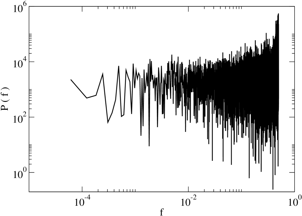
Figure 1: Log–log plot of the power spectrum of the perturbed logistic map.

Segments of the noisy, clean and filtered time series are shown in Fig. 2. In order to present all the data in the same graph, suitable constants have been added to the mean values of the signals.

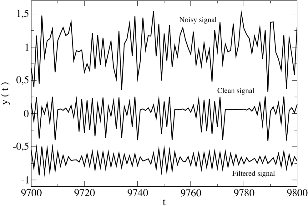
Figure 2: Noise reduction by the KNNR algorithm for a strongly perturbed logistic map.

In Fig. 3 the values of $L$ for increasing sample size are plotted. A mean squares fit of the resulting data is performed with respect to the formula

$$L_{M}=L-aM^{-\frac{1}{2}},\quad a>0.$$ (54)

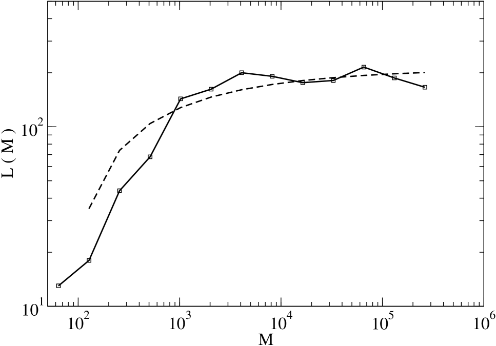
Figure 3: Convergence of $L$ for the perturbed logistic map.

The type of convergence given in Eq. (54) is suggested by the first order error term Eq. (7), in the anticipation formula of the original Bagnoli, Berrones and Franci setup. This behavior of errors is obtained for the case in which the basis components are independent random variables. The fundamental point in the derivation of Eq. (7) is that the fluctuations of these components sum in accordance to the Central Limit Theorem [1]. The numerical results suggest that for strongly chaotic systems this condition holds. In this example the number of hidden components converge to a value of order $L\sim 10^{2}$.

The convergence of $L$ constitute a basis for a novel technique of identification of chaos and other types of deterministic behavior in time series. In real world problems, the availability of arbitrarily large samples is a rare luxury. The convergence of $L$ can be however assesed indirectly, through the parameter $\alpha$ that appears in formula (49). As the sample size grows, the variance terms of Eq. (49) tend to be constant. In order to have a finite value for $L$, $\alpha$ must be decreasing with $M$. Of course, assimptotically $\alpha\propto M^{-1}$. The particular way in which this assimptotic behavior is attained is unknown. By a smootness assumption a decreasing behavior of $\alpha$ can be however expected for a range of sample sizes. Note that this claim is consistent with the curve shown in Fig. 3. On the other hand, according to the evidence presented in Subsection III-D, $L$ diverges assimptotically in a linear way with sample size for linear stochastic processes with finite correlation lengths. On these grounds, the proposed test for determinism is a standard $F$–test applied to $log[\alpha(M)]$. Consider the model $log(\alpha)=-\beta log(M)+c$, where $\beta$ is a positive number and $c$ is a real. These parameters are given by fitting the linear model to data. The null hypothesis is that $\beta=0$. Numerical results indicate that the proposed test gives a reliable identification with input signals of moderate length. In this and all of the following examples the $F$-test is performed over a set of values of the parameter $\alpha$ calculated through the KNNR algorithm for noisy signals with sample sizes of $64$, $128$, $256$, $512$, $1024$, $2048$, $4096$, $8192$ and $16384$.

In Fig. 4 is presented $log(\alpha)$ vs $log(M)$, where $log$ stands for the natural logarithm. It turns out that $F=42>>F_{0.05}(1,7)=5.59$, so the null hypothesis is clearly rejected at a $95\%$ confidence level.

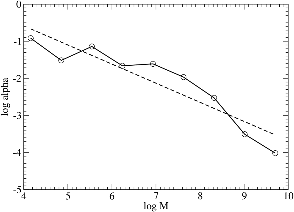
Figure 4: Behavior of $\alpha$ with increasing $M$ for the noisy logistic map.

III-B The Hénon Map

A famous two dimensional extension of the Logistic Map is the system introduced by Hénon [5],

$$s_{i}=a-s_{i-1}^{2}+bx_{i-1},$$ (55)

$$s_{i}=x_{i-1}.$$

The canonical values $a=1.4$, $b=0.3$ are taken. The iteration of the map (55) is done starting from the initial conditions $s_{0}=0.5$, $x_{0}=0.5$. The KNNR algorithm is applied to a case in presence of a noise with variance $1.2$ (the variance of the clean signal is $1$). The knowledge network algorithm performs a satisfactory noise reduction of the input signal. Fig. 5 shows the power spectrum of the clean, noisy and filtered signals in semilog scale. The input has a length of $16384$ points. The filtered signal captures the overall shape of the clean spectrum.

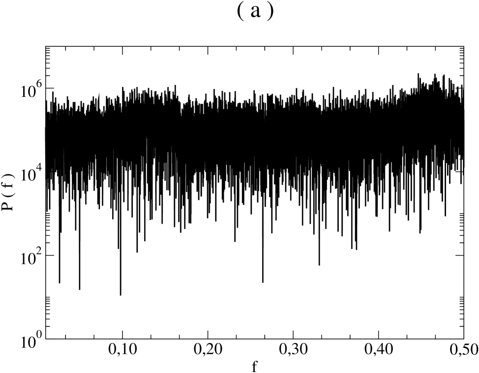
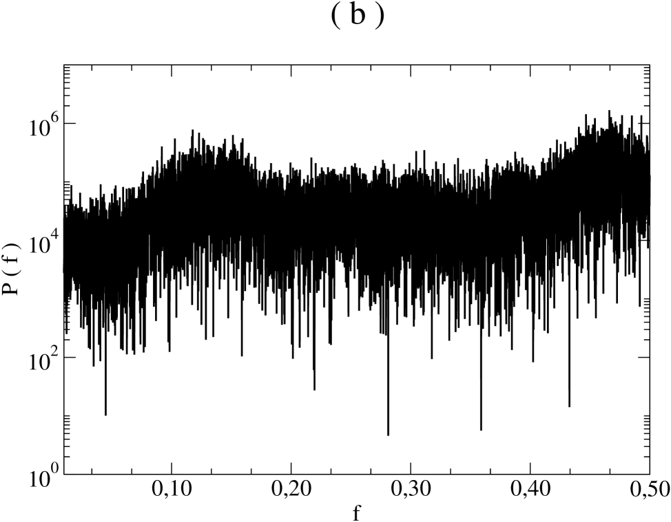
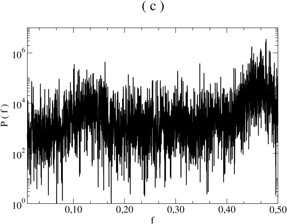
Figure 5: Semilog plots of the power spectra of a signal generated by the Hénon map: (a) noisy case, (b) clean signal, (c) filtered signal.

For the noisy Hénon system the $F$–test again indicates convergence in $L$ at a $95\%$ confidence level. It is found that $F=7.2>F_{0.05}(1,7)=5.59$.

III-C The Intermittency Map

In this example the deterministic part of the input is generated by the iteration of the intermittency map,

$$s_{i}=\beta+s_{i-1}+cs_{i-1}^{m},\quad 0<s_{i-1}\leq d$$ (56)

$$=\frac{s_{i-1}-d}{1-d},\quad d<s_{i-1}<1$$

$$c=\frac{1-\beta-d}{d^{m}}.$$

The map (56) is related to several models that arise in the study of the phenomenon of intermittency found in turbulent fluids [14]. Recently, the map (56) has been proposed as a model for the long term dynamics of packet traffic in telecommunication networks [6].

Depending on the parameters, the system (56) can display spectral properties that range from white noise to $1/f$ noise.

The values for the parameteres $m$ and $d$ considered here are $m=2$, $d=0.7$. The initial condition is taken as $0.01$. Two different cases are studied:

i) $\beta=0.05$.

With this choice of the parameters the map generates a signal with rapidly decaying correlations. The short – term correlations are reflected in the fact that the spectrum is a white noise for frequencies smaller than $\sim 0.1$, as shown in Fig. 6a. The same chaotic system in the presence of additive noise is considered in Figures 6b and 6c. The noise values are independently drawn from a Gaussian distribution with standard deviation of $0.4$ (the standard deviation of the clean signal is $0.26$). The perturbed chaotic signal enters as input in the KNNR algorithm. In Fig. 7 is shown how the KNNR algorithm is capable to reduce considerabily the noise. Morover, the filtered signal has similar spectral properties that the clean signal, despite the fact that the noisy data displays an almost flat spectrum at all frequencies.

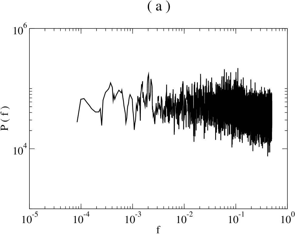
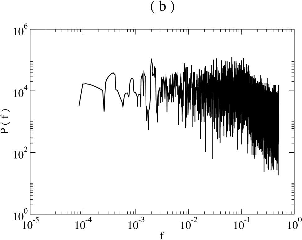
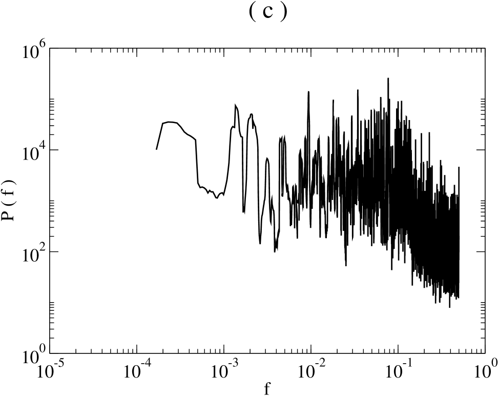
Figure 6: Log–log plots of the power spectra of a signal generated by the intermittency map ($\beta=0.05$): (a) noisy case, (b) clean signal, (c) filtered signal.

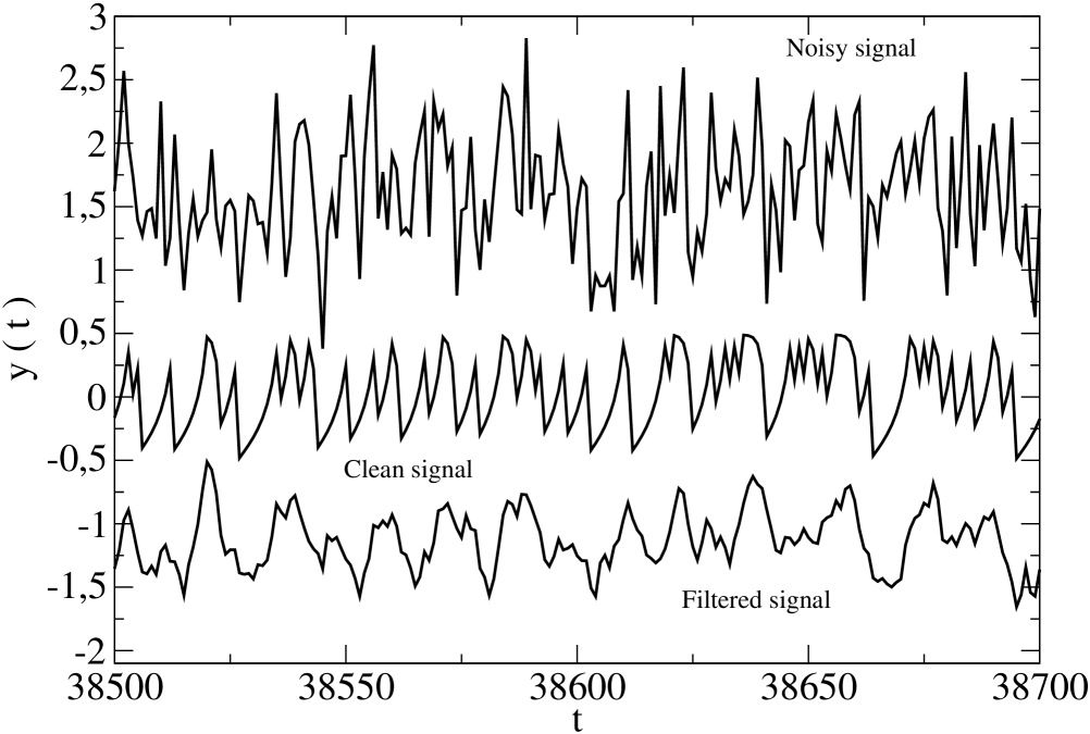
Figure 7: Noise reduction for a strongly perturbed intermittency map ($\beta=0.05$).

The behavior of $\alpha$ calculated from samples of the noisy signal with increasing sample size is shown in Fig. 8. The $F$–test gives $F=12.8>F_{0.05}(1,7)=5.59$.

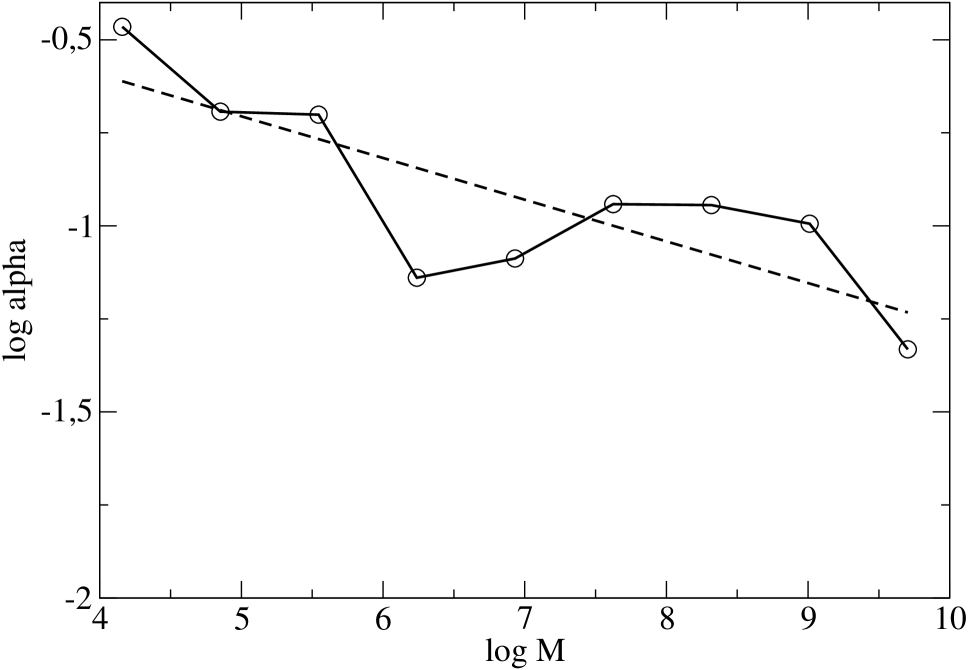
Figure 8: Behavior of $\alpha$ with increasing $M$ for the noisy intermittency map ($\beta=0.05$).

ii) $\beta=0.0005$

In this case the correlations decay much more slowly. The mean squares fit of the power spectrum of the clean signal to a power law indicates $P(f)\propto f^{-1.15}$, with a crossover to white noise at frequencies $\sim 0.001$.

Noise reduction is performed to this map in the presence of independent Gaussian perturbations, taken from a distribution with standard deviation of $0.5$, a value that almost doubles the standard deviation of the clean signal, which is $0.26$. The Fig. 9 makes clear how the KNNR algorithm is in this case capable to extract the essentially correct spectral properties from a very noisy input signal. While the noisy signal has a power spectrum described by $P(f)\propto f^{-0.3}$, which is close to the spectrum of a white noise, the fitting of the spectrum of the filtred signal to a power law indicates $P(f)\propto f^{-1.11}$.

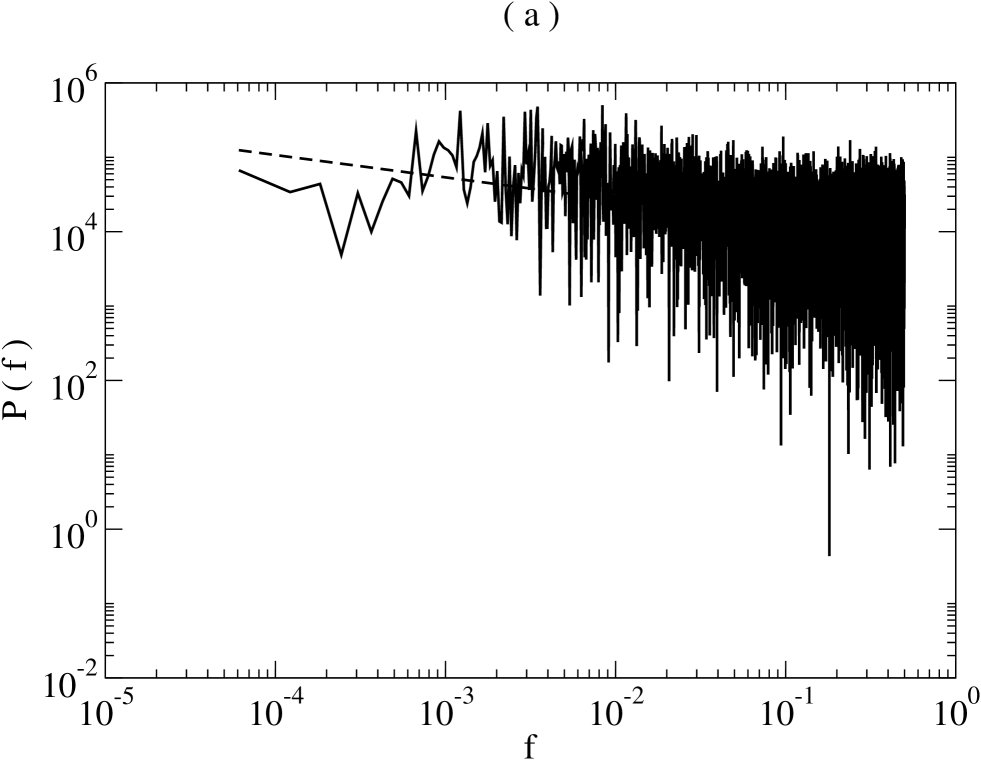
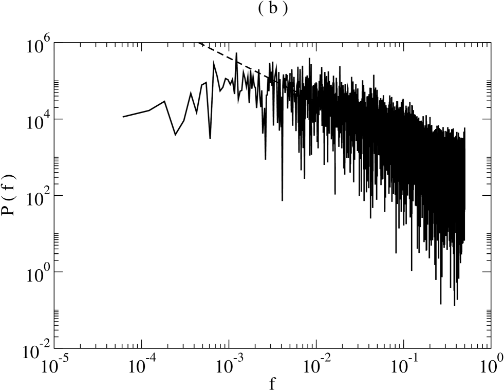
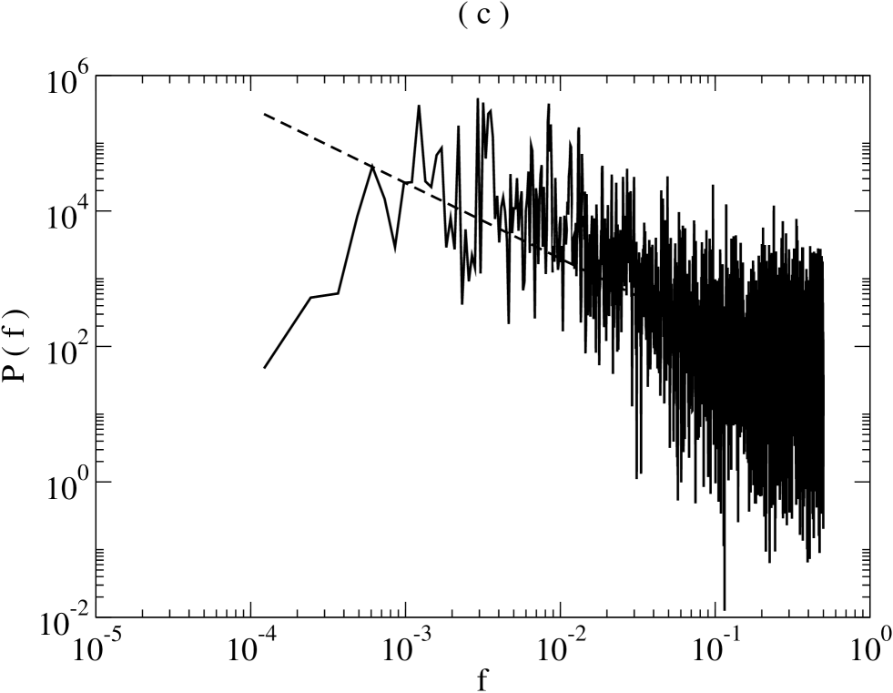
Figure 9: Log–log plots of the power spectra of a signal generated by the intermittency map ($\beta=0.0005$): (a) noisy case, (b) clean signal, (c) filtered signal. The clean and filtered signals display very similar spectral properties, while the noisy signal is close to a white noise.

The application of the $F$–test to succesive values of $\alpha$ calculated by the KNNR algorithm with the noisy signal as input, gives evidence of the convergence to a finite $L$. It is found $F=13>F_{0.05}(1,7)=5.59$.

III-D White Noise and Ornstein–Uhlenbeck Processes

In contrast to deterministic systems, even in the case that these were chaotic, stochastic systems do not display a convergence in $L$ with increasing observation time. The numerical experiments indicate that for signals generated by stochastic processes with a finite correlation length, $L$ asimptotically grows linearly with sample size.

The KNNR algorithm is applied to signals generated by discrete analogous of the white noise and Ornstein–Uhlenbeck processes: sequences of independent random numbers and the AR(1) process, respectively.

A sequence of independent Gaussian deviates is generated by the already mentioned L’Ecuyer algorithm. In Fig. 10 is presented the behavior of model complexity for a signal in which the random numbers are drawn from a distribution with standard deviation of $0.23$. The number $L$ diverge linearly. Performing an $F$-test in the same way as before (Fig. 11) gives $F=0.25<<F_{0.05}(1,7)=5.59$, which indicates that the hypothesis of a constant $\alpha$ can’t be rejected at the $95\%$ confidence level.

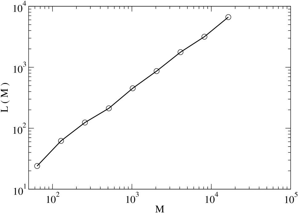
Figure 10: $L$ $vs$. $M$ for a sequence of independent random numbers. $L$ diverges linearly with sample size.

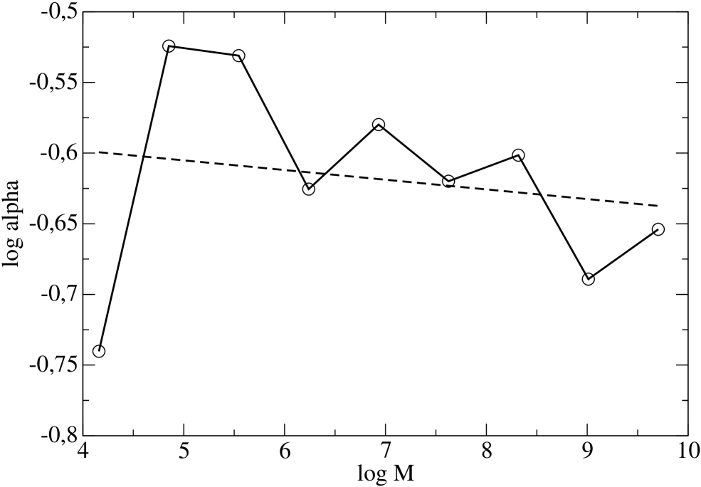
Figure 11: Behavior of $\alpha$ with increasing $M$ for a sequence of independent random numbers.

In Fig. 12 the values of $L$ for increasing sample size are plotted for three different realizations of an AR(1) process of the form

$$y_{t}=y_{t-1}-\lambda y_{t}+\varepsilon_{t},\quad 0<\lambda<1.$$ (57)

Figure 12: Behavior of $L$ with increasing $M$ for AR(1) processes with different correlation lengths.

The term $\varepsilon_{t}$ is again a Gaussian deviate generated by the L’Ecuyer algorithm with a standard deviation of $0.23$. In the limit in which the parameter $\lambda$ goes to zero the process (57) tends to a random walk. For other values of $\lambda$ the correlations decay exponentially, with a characteristic time $1/\lambda$. The examples considered in Fig. 12 have the parameter values $\lambda=0.5$, $\lambda=0.05$ and $\lambda=0.005$. Note that $L$ eventually diverges linearly for all cases. The point at which this divergent regime is attained depends on the correlation length. In fact, the $F$–test performed for a maximum sample size of $16384$ rejects the null hypothesis at a $95\%$ confidence level only in the first two cases. This implies that for small enough samples, linear autocorrelated stochastic processes are indistinguishable by the KNNR algorithm from chaotic sistems with similar autocorrelations. This is quite natural taking into account that the KNNR algorithm is based on the linear autocorrelation structure. It must be pointed out however, that if the stochastic signal at hands has finite correlation length, the numerical experiments suggest that the identification of determinism is always possible with large enough sample sizes.

It’s worth mention that in all of the examples in this Subsection, the filtered signals display the same correlation lengths than the original signals.

IV Conclusion

The proposed formalism constitute a basis for a novel technique of identification of deterministic behavior in time series. A careful study of the convergence of $L$ as the sample size grows, may be used to improve the introduced statistical test. The question of the definition of the most adequate statistic and test to be used, e. g. parametric or non–parametric, deserves further research. In the same direction, statistical tests could also be made on the basis of a comparision between the spectral properties of a signal before and after its filtering by the KNNR algorithm.

The presented results, on the other hand, give a linear filter for noise reduction capable to extract features otherwise difficult to deduce from traditional linear approches. Further research should be done on the use of the KNNR algorithm for noise reduction and forecasting in important fields of application.

The presented approach treats the time series in a very direct manner. The generalization of the KNNR algorithm to the case in which $y$ depends on more than one variable could be used to allow delay representations of data. This may give a more powerful algorithm, capable to identify deterministic behavior in smaller data sets, and to connect the presented theory with the important problem of the calculation of embedding dimensions. This generalization of the study to higher dimensional data sets could also find application in questions such like the estimation of the optimal number of hidden neurons in models of artificial neural networks.

References

- [1] F. Bagnoli, A. Berrones and F. Franci, “Degustibus Disputandum (Forecasting Opinions by Knowledge Networks)”, Physica A 332, 2004, pp. 509-518.
- [2] M. Barahona and C. Poon, “ Detection of Nonlinear Dynamics in Short, Noisy Time Series: ”, Nature 381, 1996, pp. 215-217.
- [3] A. Berrones, “Filtering by Sparsely Connected Networks Under the Presence of Strong Additive Noise”, to be published in Proc. Seventh Mexican International Conference on Computer Science (ENC06).
- [4] S. Haykin, Neural Networks: a Comprehensive Foundation, Prentice Hall, 1999.
- [5] M. Hénon, “A Two–Dimensional Mapping with a Strange Attractor”, Commun. Math. Phys. 50, 1976, 69.
- [6] A. Herramilli, R. Singh and P. Pruthi “Chaotic Maps as Models of Packet Traffic”, Proc. 14th Int. Teletraffic Cong. 35, Elsevier, 1994.
- [7] H. Kantz and T. Schreiber, Nonlinear Time Series Analysis. Cambridge University Press, 2004.
- [8] S. Maslov and Y. Zhang, “Extracting Hidden Information from Knowledge Networks”, Physical Review Letters 87, 2001, 248701.
- [9] S. Maslov and K. Sneppen, “Specificity and Stability in Topology of Protein Networks”, Science 296, 2002, 910.
- [10] E. Ott, Chaos in Dynamical Systems. Cambridge University Press, 1993.
- [11] W. H. Press, S. A. Teukolsky, W. T. Vetterling and B. P. Flannery, Numerical Recipes in C++. The Art of Scientific Computing, 2nd ed. Cambridge University Press, 2002.
- [12] O. Renaud, J. Starck and F. Murtagh, “Wavelet–Based Combined Signal Filtering and Prediction”, IEEE Transactions on Systems, Man and Cybernetics–Part B 35, 2005, pp. 1241-1251.
- [13] C. E. Shannon and W. Weaver, The Mathematical Theory of Information, University of Illinois Press, 1949.
- [14] H. G. Schuster Deterministic Chaos: An Introduction, 2nd revised ed. VCH, 1988.
- [15] J. Theiler, S. Eubank, A. Longtin, B. Galdrikian, and J. D. Farmer, “Testing for Nonlinearity in Time Series: the Method of Surrogate Data”, Physica D 58, 1992, pp. 77-94.
- [16] N. Wiener, Cybernetics: Or the Control and Communication in the Animal and the Machine, 2nd ed. MIT Press, 1965.