Fear and its implications for stock markets

Abstract

The value of stocks, indices and other assets, are examples of stochastic processes with unpredictable dynamics. In this paper, we discuss asymmetries in short term price movements that can not be associated with a long term positive trend. These empirical asymmetries predict that stock index drops are more common on a relatively short time scale than the corresponding raises. We present several empirical examples of such asymmetries. Furthermore, a simple model featuring occasional short periods of synchronized dropping prices for all stocks constituting the index is introduced with the aim of explaining these facts. The collective negative price movements are imagined triggered by external factors in our society, as well as internal to the economy, that create fear of the future among investors. This is parameterized by a “fear factor” defining the frequency of synchronized events. It is demonstrated that such a simple fear factor model can reproduce several empirical facts concerning index asymmetries. It is also pointed out that in its simplest form, the model has certain shortcomings.

I Introduction and Motivation

Extreme events such as the September 11, 2001 attack on New York city are known to trigger rather systematically collapses in most sectors of the economy. This does not happen because fundamental factors in the economic system have worsened as a whole (from one day to another), but because the prospects of the immediate future are considered highly unknown. Investors simply fear for the future consequences of such dramatic events, which is reflected in dropping share prices. In other words, the share prices of a large fraction of stocks show collectively a negative development shortly after such a major triggering event AsymPaper .

These facts are rather well known, and one may give several other similar examples. Fortunately, such extreme events are not very frequent. One should therefore expect that collective draw-downs are rare. On the contrary, we find that they are much more frequent than one would have anticipated. One may say there is a sequence of “mini-crashes” characterized by synchronized downward asset price movements. As a consequence it is consistently more probable — up to a well defined (short) timescale — to loose a certain percentage of an investment placed in indices, than gaining the same amount over the same time interval. This is what we call a gain-loss asymmetry and it has been observed in different stock indices including the Dow Jones Industrial Average (DJIA), the SP500 and NASDAQ Johansen , but not, for instance, in foreign exchange data invfx .

In this paper we will briefly revisit some of the empirical facts of the gain-loss asymmetry. Then we suggest an explanation of the phenomenon by introducing a simple (fear factor) model. The model incorporates the concept of a synchronized event, among the otherwise uncorrelated stocks that compose the index. This effect is seen as a consequence of risk aversion (or fear for the future) among the investors triggered by factors external, as well as internal, to the market. In our interpretation, the results show that the concept of fear has a deeper and more profound consequence on the dynamics of the stock market than one might have initially anticipated.

II The inverse statistics approach

A new statistical method, known as inverse statistics has recently been introduced Mogens ; optihori ; gainloss ; invfx . In economics, it represents a time-dependent measure of the performance of an asset. Let $S(t)$ denote the asset price at time $t$. The logarithmic return at time $t$, calculated over a time interval $\Delta t$, is defined as Book:Bouchaud-2000 ; Book:Mantegna-2000 ; Book:Hull-2000 $r_{\Delta t}(t)=s(t+\Delta t)-s(t)$, where $s(t)=\ln S(t)$. We consider a situation in which an investor aims at a given return level, $\rho$, that may be positive (being “long” on the market) or negative (being “short” on the market). If the investment is made at time $t$ the inverse statistics, also known as the investment horizon, is defined as the shortest time interval $\tau_{\rho}(t)=\Delta t$ fulfilling the inequality $r_{\Delta t}(t)\geq\rho$ when $\rho\geq 0$, or $r_{\Delta t}(t)\leq\rho$ when $\rho<0$.

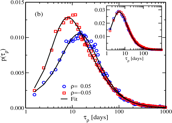
(a) The empirical results for the DJIA.

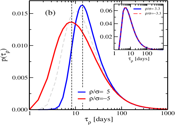
(b) The results for the fear factor model.

Figure 1: (Color online) The inverse statistics distributions : (a) The panel shows histograms of the inverse statistics for the DJIA obtained on the basis of the empirical daily close data covering its entire history of 110 years from 1896. The red open squares are obtained using a loss level of $\rho=-0.05$ and the blue open circles are obtained using a gain level of $\rho=+0.05$ and both distributions are normalized. Note the clear asymmetry between the loss and the gain statistics. The full curves are regression fits using a generalized inverse Gamma distribution optihori ; gainloss ; invfx . The inset shows the distributions obtained from using the same procedure on the individual stocks of the DJIA, and subsequently averaging over the stocks. Notice that the asymmetry is absent for individual stocks. (b) The results for the inverse statistics obtained within the fear factor model applying parameters characterizing the DJIA and used to produce the empirical results of Fig. 1(a). In particular it was used that the index consists of $N=30$ stocks and the return level was set to $\rho/\sigma=5$, where $\rho$ is the return level and $\sigma$ denotes the daily volatility of the index. In the model the index volatility, $\sigma$, should reflect the observed $1$% daily volatility of the DJIA, and the $\rho/\sigma=\pm 5$ therefore corresponds to $\rho=\pm 5$% in Fig. 1(a). A fear factor of $p=0.05$ was chosen to reproduce the positions of the two asymmetric maxima appearing in Fig. 1(a) and indicated by dashed vertical lines. The dashed thick line is the result for a fear-factor parameter $p=0$, in which case the asymmetry vanishes. As in Fig. 1(a), the inset shows the loss and gain distributions for the individual stocks in the model. Notice, that here the asymmetry is also absent.

The inverse statistics histogram, or in economics, the investment horizon distribution, $p\left(\tau_{\rho}\right)$, is the distribution of all available waiting times $\tau_{\rho}(t)$ obtained by moving through time $t$ of the time series to be analyzed (Fig. 1(a)). Notice that these methods, unlike the return distribution approach, do not require that data are equidistantly sampled. It is therefore well suited for tick-to-tick data.

If the return level $\rho$ is not too small the distribution $p\left(\tau_{\rho}\right)$ has a well defined maximum, see Fig. 1(a). This occurs because it takes time to drive prices through a certain level. The most probable (waiting) time, i.e. the maximum of the distribution, corresponds to what has been termed the optimal investment horizon optihori for a given return level, $\rho$, and will be denoted $\tau_{\rho}^{*}$ below.

III Empirical results

In this section, we present some empirical results on the inverse statistics. The data set used is the daily close of the DJIA covering its entire history from 1896 till today. Fig. 1(a) depicts the empirical inverse statistics histograms — the investment horizon distribution — for (logarithmic) return levels of $\rho=0.05$ (open blue circles) and $\rho=-0.05$ (open red squares). The histograms possess well defined and pronounced maxima, the optimal investment horizons, followed by long $1/t^{3/2}$ power-law tails that are well understood Book:Bouchaud-2000 ; Book:Mantegna-2000 ; Book:Hull-2000 ; Book:Johnson-2003 . The solid lines in Fig. 1(a) represent generalized inverse Gamma distributions optihori fitted towards the empirical histograms. This particular functional form is a natural candidate since it can be shown that the investment horizon distribution is an inverse Gamma distribution , $p(x)\sim{\rm exp}(a/2x)/x^{3/2}$ ($a$ being a parameter), if the analyzed asset price process is (a pure) geometrical Brownian motion Book:Karlin-1966 ; Book:Redner-2001 .

A striking feature of Fig. 1(a) is that the optimal investment horizons with equivalent magnitude of return level, but opposite signs, are different. Thus the market as a whole, monitored by the DJIA, exhibits a fundamental gain-loss asymmetry. As mentioned above other indices, such as SP500 and NASDAQ, also show this asymmetry Johansen , while, for instance, foreign exchange data do not invfx .

It is even more surprising that a similar well-pronounced asymmetry is not found for any of the individual stocks constituting the DJIA Johansen . This can be observed from the insert of Fig. 1(a), which shows the results of applying the same procedure, individually, to these stocks, and subsequently averaging to improve statistics.

Fig. 2(a) depicts the empirical dependence of the optimal investment horizon (the maximum of the distribution), $\tau_{\rho}^{*}$, as a function of the return level $\rho$. If the underlying stochastic price process is a geometrical Brownian motion, then one can show that $\tau_{\rho}^{*}\sim\left|\rho\right|^{\gamma}$, with $\gamma=2$, valid for all return levels $\rho$ (indicated by the lower dashed line in Fig. 2(a)). Instead one empirically observes a different behavior with a weak ($\gamma\approx 0$), or no, dependence on the return level when it is small compared to the (daily) volatility, $\sigma$, of the index. For instance the DJIA daily volatility is about $\sigma_{\tiny DJIA}\approx 1$%. On the other hand a cross-over can be observed, for values of $\rho$ somewhat larger than $\sigma$, to a regime where the exponent $\gamma$ is in the range of $1.8$–$2$. Based on the empirical findings we do not insist on a power-law dependence of $\tau_{\rho}^{*}$ on $\rho$. The statistics is too poor to conclude on this issue, and there seem to be even some $\rho$ dependence in $\gamma$. Other groups though ZhouYuan ; Poland , have found indications of similar power-law behavior in both emerging and liquid markets supporting our findings. An additional interesting and apparent feature to notice from Fig. 2(a) is the consistent, almost constant, relative gain-loss asymmetry in a significant wide range of return levels.

In light of these empirical findings the following interesting and fundamental question arises: Why does the index exhibit a pronounced asymmetry, while the individual stocks do not? This question is addressed by the model introduced below.

IV The fear factor model

Recently the present authors introduced a so-called fear factor model in order to explain the empirical gain-loss asymmetry AsymPaper . The main idea is the presence of occasional, short periods of dropping stock prices synchronized between all $N$ stocks contained in the stock index. In essence these collective drops are the cause (in the model) of the asymmetry in the index AsymPaper . We rationalize such behavior with the emergence of anxiety and fear among investors. Since we are mainly interested in day-to-day behavior of the market, it will be assumed that the stochastic processes of the stocks are all equivalent and consistent with a geometrical Brownian motion Book:Bouchaud-2000 ; Book:Mantegna-2000 ; farmer . This implies that the logarithm of the stock prices, $s_{i}(t)=\ln S_{i}(t)$, follow standard, unbiased, random walks

$$s_{i}(t+1)=s_{i}(t)+\varepsilon_{i}(t)\delta\;,\qquad i=1,\ldots,N,$$ (1)

where $\delta>0$ denotes the common fixed log-price increment (by assumption), and $\varepsilon_{i}(t)=\pm 1$ is a random time-dependent direction variable. At certain time steps, chosen randomly with fear factor probability $p$, all stocks synchronize a collective draw down ($\varepsilon_{i}=-1$). For the remaining time steps, the different stocks move independently of one another. To assure that the overall dynamics of every stock is behaving equivalent to a geometric Brownian motion, a slight upward drift, quantified by the probability for a stock to move up $q=1/(2(1-p))$ AsymPaper , is introduced. This “compensating” drift only governs the non-synchronized periods. ¿From the price realizations of the $N$ single stocks, one may construct the corresponding price-weighted index, like in the DJIA, according to

$$I(t)=\frac{1}{d(t)}\sum_{i=1}^{N}S_{i}(t)\;=\;\frac{1}{d(t)}\sum_{i=1}^{N}\exp\{s_{i}(t)\}\;.$$ (2)

Here $d(t)$ denotes the divisor of the index at time $t$ that for simplicity has been fixed to the value $d(t)=N$. Some consideration is needed when choosing the value of $\delta$. If $\delta$ is too small the daily index volatility will not be large enough to reach the return barrier $\rho$ within an appropriate time. On the other hand, when $\delta$ is too large it will cause a crossing of the negative return barrier no later than the first occurring synchronous step (if $\left|\rho\right|$ is not too large). Under such circumstances, the optimal investment horizon for negative returns ($\tau_{-\left|\rho\right|}^{*}$) will only to a very little extent depend on $\rho$ which is inconsistent with empirical observations. Therefore, the parameter $\delta$ should be chosen large enough, relative to $\left|\rho\right|$, to cause the asymmetry, but not too large to dominate fully whenever a synchronous step occurs. A balanced two-state system is the working mechanism of the model — dominating calm behavior interrupted by short-lived bursts of fear. For more technical details on the model, the interested reader is referred to Ref. AsymPaper .

It is important to realize that the asymmetric investment horizons obtained with the model stems from the very simple synchronization events between stocks isolated in time, and not by means of higher-order correlations. The cause of these simultaneous drawdowns could be both internal and external to the market, but no such distinctions are needed to create the dynamics and asymmetry of the fear factor model. This differs — at least model wise — the inverse statistics asymmetry from the leverage phenomenon reported in e.g. BouchaudLeverage and elsewhere. Though the two phenomena conceptually are related, the asymmetric gain-loss horizons can be simulated without involving complex stochastic volatility models.

The minimalism of the model also involves aspects that are not entirely realistic. Work is in progress to extend the model by including features of more realistic origin. In particular, we have included splittings, mergers and replacements as well as selected economic sectors which have their own fear factors. Moreover, other extensions include more realistic (fat-tailed) price increment distributions Book:Bouchaud-2000 ; Book:Mantegna-2000 ; Book:Hull-2000 ; mandelbrot62 as well as time-dependent stochastic volatility for the single stocks engle ; engle-patton ; Book:Bouchaud-2000 ; Book:Mantegna-2000 ; Book:Hull-2000 . The detailed results of these extensions will be reported elsewhere FurtherWork .

V Results and discussion

We will now address the results that can be obtained by the fear factor model and compare them with the empirical findings. Fig. 1(b) shows that the model indeed produces a clear gain-loss asymmetry in the inverse statistic histograms. Hence, the main goal of the model is obtained. Moreover, the investment horizon distributions are qualitatively very similar to what is found empirically for the DJIA (cf. Fig. 1(a)). In particular, one observes from Fig. 1(b) that the positions of the peaks found empirically (vertical dashed lines) are predicted rather accurately by the model. To produce the results of Fig. 1(b), a fear factor of $p=0.05$ was used. Furthermore it is observed, as expected, that the model with $p=0$ does not produce any asymmetry (grey dashed line in Fig. 1(b)).

A detailed comparison of the shapes of the empirical and the modelled inverse statistics distribution curves reveal some minor differences, especially regarding short waiting times and the height of the $\rho>0$ histogram. One could find simple explanations for these differences, such as the fact that the model does not consider a realistic jump size distribution, or even that it does not include an “optimism factor” synchronizing draw-ups. This would result in a wider $\rho>0$ distribution for short waiting times, and additionally would lower the value of the maximum. Some of these shortcomings of the minimalistic model has already been dealt with in Ref.  FurtherWork . For the sake of this paper, however, none of these extension will be further discussed in detail.

Fig. 2(b) depicts the optimal investment horizon vs. return level obtained from our fear factor model. It is observed that for $\rho>0$ the empirical result for the DJIA (solid line in Fig. 2(b)) is reasonably well reproduced. One exception is for the largest return levels, where a value of $\gamma=2$ seems to be asymptotically approached. This might not be so unexpected since this is the geometric Brownian motion value. However, the case is different for $\rho<0$. Here the empirical behavior is not reproduced that accurately. Consistent with empirical findings, a gain-loss asymmetry gap, $\tau_{+\left|\rho\right|}^{*}-\tau_{-\left|\rho\right|}^{*}$, opens up for return levels $\rho$ comparable to the volatility of the index $\sigma$. Unlike empirical observed results (Fig. 2(a)), the gap, however, decreases for larger return levels. The numerical data seems also to indicate that the closing of the gain-loss asymmetry gap results in a data collapse to a universal $\tau_{\rho}^{*}\sim\rho^{\gamma}$ curve with exponent $\gamma=2$.

We will now argue why this is a plausible scenario. Even during a synchronous event, when all stocks drop simultaneously, there is a upper limit on the drop of the index value. One can readily show (cf. Eq. (4) of Ref. AsymPaper ) that the relative returns of the index during a synchronous event occurring at $t+1$ is

$$\frac{\Delta I(t)}{I(t)}=\frac{I(t+1)-I(t)}{I(t)}=\exp(-\delta)-1<0,$$ (3)

which also is a good approximation to the corresponding logarithmic return as long as $I(t)\gg\Delta I(t)$ Book:Mantegna-2000 . This synchronous index drop sets a scale for the problem. One has essentially three different regions, all with different properties, depending on the applied level of return. They are characterized by the return level $\rho$ being (i) much smaller than; (ii) comparable to; or (iii) much larger than the synchronous index drop $\exp(-\delta)-1$. In case (i), the synchronization does not result in a pronounced effect, and there is essentially no dependence on the return level or its sign. For the intermediate range, where $\rho$ is comparable to $\exp(-\delta)-1$, the asymmetric effect is pronounced since no equivalent positive returns are very probable for the index (unless the fear factor is very small). Specifically, whenever $\rho<\exp(-\delta)-1$ one collective draw-down event is sufficient to cross the lower barrier of the index, thereby resulting in an exit time coinciding with the time of the synchronization. Of course this is not the case when $\rho>0$ giving the working mechanism in the model for the asymmetry at short time scales. For the final case, where $\rho\gg\exp(-\delta)-1$, neither the synchronized downward movements, or the sign of the return level, play an important role for the barrier crossing. However, in contrast to case (i) above, the waiting times are now much longer, so that the geometrical Brownian character of the stock process is observed. This is reflected in Fig. 2(b) by the collapse onto an apparent common scaling behavior with $\gamma=2$ independent of the sign of the return level.

The last topic to be addressed in this paper is also related to an asymmetry, but takes a somewhat different shape from what was previously considered. By studying the probability that the DJIA index decreases, respectively increases, from day to day, we have found a $9\%$ larger probability for the index to decrease rather than increase. This information led us to a more systematic study by considering the number of consecutive time steps, $n_{t}$, the index drops or raises. This probability distribution will be denoted by $p_{\pm}(n_{t})$, where the subscripts $+/-$ refers to price raise/drop. The open symbols of Fig. 3 show that the empirical results, based on daily DJIA data, are consistent with decaying exponentials of the form $p_{\pm}(n_{t})\sim\exp(-\gamma_{\pm}\left|n_{t}\right|)$, where $\gamma_{\pm}>0$ are parameters (or rates). It is surprising to observe that also this measure exhibits an asymmetry since $\gamma_{+}\neq\gamma_{-}$. These rates, obtained by exponential regression fits to the empirical DJIA data, are $\gamma_{+}=(0.62\pm 0.01)\,\mbox{days}^{-1}$ and $\gamma_{-}=(0.74\pm 0.03)\,\mbox{days}^{-1}$. What does the fear factor model, indicate for the same probabilities? In Fig. 3 the dashed lines are the predictions of the model and they reproduce the empirical facts surprisingly well. They correspond to the following parameters $\gamma_{+}=0.62\,\mbox{days}^{-1}$ and $\gamma_{-}=0.78\,\mbox{days}^{-1}$ for the raise and drop curves, respectively. However, the value of the fear factor necessary to obtain these results was $p=0.02$. This is slightly lower than the value giving consistent results for the inverse statistics histograms of Figs. 2. In this respect, the model has an obvious deficiency. It should be stressed, though, that it is a highly non-trivial task, with one adjustable parameter, to reproduce correctly the two different rates ($\gamma_{\pm}$) for the two probabilities. That such a good quantitative agreement with real data is possible must be seen as a strength of the presented model.

VI Conclusions and outlooks

In conclusion, we have briefly reviewed what seems to be a new stylized fact for stock indices that show a pronounced gain-loss asymmetry. We have described a so-called minimalistic “fear factor” model that conceptually attributes this phenomenon to occasional synchronizations of the composing stocks during some (short) time periods due to fear emerging spontaneously among investors likely triggered by external world events. This minimalistic model do represent a possible mechanism for the gain-loss asymmetry, and it reproduces many of the empirical facts of the inverse statistics.

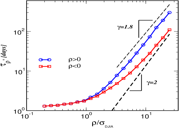
(a) The empirical results for the DJIA.

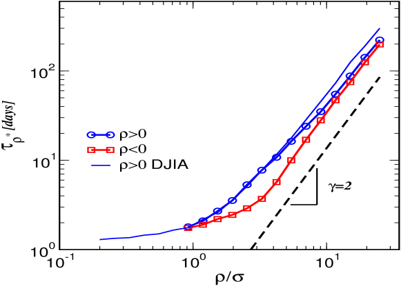
(b) The results for the fear factor model.

Figure 2: The dependence of the optimal investment horizon on the return level (scaled with the daily volatility): (a) The DJIA empirical optimal investment horizon $\tau^{*}_{\rho}$ for positive (open circles) and negative (open squares) levels of return $\pm\rho$. The daily volatility used for the rescaling was $\sigma_{\mbox{\tiny DJIA}}\approx 1\%$. In the case where $\rho<0$ one has used $-\rho$ on the abscissa for reasons of comparison. If a geometrical Brownian price process is assumed, one will have $\tau^{*}_{\rho}\sim\rho^{\gamma}$ with $\gamma=2$ for all values of $\rho$. Such a scaling behavior is indicated by the lower dashed line in the graph. Empirically one finds values of $\gamma\simeq 1.8$ (upper dashed line), but only for large values of the return. (b) Results of the fear factor model analog to the empirical DJIA results of Fig. 2(a). The parameters used to produce the model results of this figure were those given in the caption of Fig. 1.

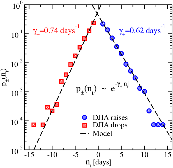
Figure 3: (Color online) The distribution, $p_{\pm}(n_{t})$, of the number of consecutive days in a row, $n_{t}$, the DJIA index is dropping (filled red squares) or raising (filled blue circles squares). We have adopted the convention that drops correspond to negative values of $n_{t}$ while raises correspond to positive. The exponential rates $\gamma_{\pm}$ for the empirical DJIA data were determined by regression to $\gamma_{+}=(0.62\pm 0.01)\,\mbox{days}^{-1}$ and $\gamma_{-}=(0.74\pm 0.03)\,\mbox{days}^{-1}$. The dashed lines correspond to the prediction of the fear factor model using the parameters of Fig. 1 except that the fear factor was lowered slightly ($p=0.02$). Notice that only one single parameter, the fear factor $p$, had to be adjusted in order to correctly reproduce the two empirical rates.

References

- (1) R. Donangelo, M.H. Jensen, I. Simonsen, and K. Sneppen, Synchronization Model for Stock Market Asymmetry, preprint arXiv:physics/0604137 (2006). To appear in J. Stat. Mech.: Theor. Exp.
- (2) A. Johansen, I. Simonsen, and M.H. Jensen, Optimal Investment Horizons for Stocks and Markets, preprint, 2005.
- (3) M.H. Jensen, A. Johansen, F. Petroni, and I. Simonsen, Physica A 340, 678-684 (2004).
- (4) M.H. Jensen, Phys. Rev. Lett. 83, 76-79 (1999).
- (5) I. Simonsen, M.H. Jensen, and A. Johansen, Optimal Investment Horizons Eur. Phys. Journ. 27, 583-586 (2002).
- (6) M.H. Jensen, A. Johansen, and I. Simonsen, Physica A 324, 338-343 (2003).
- (7) J.-P. Bouchaud and M. Potters, Theory of Financial Risks: From Statistical Physics to Risk Management (Cambridge University Press, Cambridge, 2000).
- (8) R.N. Mantegna and H.E. Stanley, An Introduction to Econophysics: Correlations and Complexity in Finance (Cambridge University Press, Cambridge, 2000).
- (9) J. Hull, Options, Futures, and other Derivatives, 4th ed. (Prentice-Hall, London, 2000).
- (10) N.F. Johnson, P. Jefferies, and P.M. Hui, Financial Market Complexity (Oxford University Press, 2003).
- (11) Karlin, S. A First Course in Stochastic Processes (Academic Press, New York, 1966).
- (12) S. Redner, A Guide to First Passage Processes (Cambridge, New York, 2001).
- (13) W.-X. Zhou and W.-K. Yuan, Physica A 353 433-444 (2005).
- (14) M. Zaluska-Kotur, K. Karpio and A. Orlowski, Acta Phys. Pol. B 37, 3187-3192 (2006); K. Karpio, M. Zaluska-Kotur and A. Orlowski, Physica A, in press (2006).
- (15) D. Farmer, Comp. Sci. Eng. 1 (6) 26-39, (1999).
- (16) J.-P. Bouchaud, A. Matacz and M. Potters, Phys. Rev. Lett. 87, 228701-1-4 (2001).
- (17) B. Mandelbrot, J. Bus. 36, 307-332 (1963).
- (18) R.F. Engle, Econometrica 61, 987 (1982).
- (19) R.F. Engle, and A.J. Patton, Quant. Fin. 1, 237 (2001).
- (20) P.T.H. Ahlgren, M.H. Jensen and I. Simonsen, Unpublished work (2006).