Robust, High-speed, All-Optical Atomic Magnetometer

Abstract

A self-oscillating magnetometer based on the nonlinear magneto-optical rotation effect with separate modulated pump and unmodulated probe beams is demonstrated. This device possesses a bandwidth exceeding $1\,{\rm kHz}$. Pump and probe are delivered by optical fiber, facilitating miniaturization and modularization. The magnetometer has been operated both with vertical-cavity surface-emitting lasers (VCSELs), which are well suited to portable applications, and with conventional edge-emitting diode lasers. A sensitivity of around $3\,{\rm nG}$ is achieved for a measurement time of $1\,{\rm s}$.

I Introduction

Considerable progress has been made in recent years in atomic magnetometry, including the achievement of subfemtotesla sensitivity Kominis2003 , the application of coherent dark states to magnetometry Nagel1998 ; Affolderbach2002 , development of sensitive atomic magnetometers for biological applications Bison2003 ; Xia2006 and for fundamental physics murthy1989 ; berglund1995 ; youdin1996 ; romalis2001 ; amini2003 ; Groeger2006 , the introduction of chip-scale atomic magnetometers schwindt2004 , and the development of nonlinear magneto-optical rotation (NMOR) using modulated light Budker2000 with its subsequent demonstration in the geomagnetic field range Ledbetter2006 . An important potential application is to space-based measurements, including measurements of planetary fields, of the solar-wind current, and of magnetic fields in deep space acuna2002 . As these sensitive magnetometric techniques move from the laboratory to applications in the field and in space, significant new demands will naturally be placed on their robustness, size, weight, and power consumption. An attractive approach that addresses many of these demands is the self-oscillating magnetometer configuration, originally proposed by Bloom Bloom1962 . In this configuration, the detected optical signal at the Larmor frequency or a harmonic, is used to drive the magnetic resonance, either with RF coils or, as in the present work, by optical excitation of the resonance. When this resonant drive is amplified sufficiently, the oscillation builds up spontaneously (seeded by noise) at the resonant frequency. The spontaneous nature of the oscillation obviates the necessity of slow preliminary scans, which would otherwise be required to search for the resonance and lock to the desired line. Moreover, the size, weight, and power consumption of a self-oscillating device all benefit from the simplification of the electronics that results from not requiring a local oscillator or lock-in amplifier.

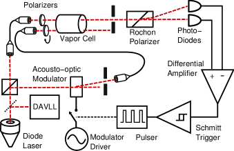
Figure 1: Diagram of experimental setup. The output of a diode laser is split into pump and probe beams. The laser is frequency-stabilized approximately $300\,{\rm MHz}$ below the center of the ⁸⁷Rb D2 Doppler-broadened line center via a dichroic atomic vapor laser lock (DAVLL). The pump beam is amplitude-modulated by an acousto-optic modulator (AOM). Both pump and probe are delivered by optical fiber to a paraffin-coated vapor cell. Separate polarizers allow independent control of pump and probe polarization. The polarization rotation of the probe beam is analyzed in a balanced polarimeter consisting of a Rochon polarizer followed by a pair of photodiodes and an amplifier. A zero-crossing detector (Schmitt trigger) and pulser control the pump power via the AOM, closing the loop and sustaining self-oscillation. In an alternate configuration, separate VCSELs on the ⁸⁷Rb D1 F=2 line supplied light for pump and probe.

A self-oscillating magnetometer based on NMOR was recently reported by Schwindt et al. schwindt2005 , in whose work the functions of pumping and probing were fulfilled by a single frequency-modulated laser beam. As a result, the detected signal was a product both of the rotating atomic alignment and of the modulated detuning, resulting in a complicated waveform that required significant electronic processing before being suitable for feeding back to the laser modulation, as required in the self-oscillating scheme.

In the present paper, we present a simple alternative arrangement that avoids many of the difficulties encountered in the single-beam experiment. Indeed, by the use of two laser beams–a modulated pump and an unmodulated probe–the optical-rotation signal may be made accurately sinusoidal, avoiding the complexity of digital or other variable-frequency filters in the feedback loop. Importantly, the use of two beams also permits optical adjustment of the relative phase of the detected signal and the driving modulation by changing the angle between their respective linear polarizations. For magnetometry at large bias field and requiring a wide range of fields, this optical tuning of the feedback-loop phase promises both good long-term stability and much greater uniformity with respect to frequency than can readily be obtained with an electronic phase shift.

II NMOR Resonance

Detailed discussions of zero-field NMOR resonances Budker1998 ; Budker2000 , as well as of the additional finite-field resonances that occur when the pumping laser light is frequency-modulated (FM) Budker2002 or amplitude-modulated (AM) Gawlik2006 , have been presented in prior work. An NMOR resonance occurs when optical pumping causes an atomic vapor to become dichroic (or birefringent), so that subsequent probe light experiences polarization rotation. For the resonances considered in this work, both pump and probe are linearly polarized and therefore primarily produce and detect atomic alignment ($\Delta m=2$ coherences). The magnetic-field dependence originates from the fact that the atomic spins undergo Larmor precession, so that weak optical pumping can only produce a macroscopic alignment when the Larmor precession frequency is small compared to the spin relaxation rate, or alternatively when pumping is nearly synchronous with precession, as in FM or AM NMOR.

If the optical-pumping rate is modulated at a frequency $\nu$, then the optical-rotation angle of the probe polarization will in general also oscillate at frequency $\nu$. If this frequency is scanned across the resonance (in open-loop configuration, i.e. with no feedback from the optical-rotation signal), then the NMOR resonance will manifest itself as a resonant peak in the rotation-angle amplitude of the probe polarization on the output. Assuming the in-going probe and pump polarizations to be parallel, the amplitude and phase of the observed rotation signal can be described by the complex Lorentzian $(\delta-i\gamma/2)^{-1}$, where $\delta\equiv 2\pi(\nu-2\nu_{\rm L})$ is the detuning from resonance, $\gamma$ is the full width (in modulation frequency) at half maximum of the resonance, and $\nu_{\rm L}$ is the Larmor frequency. The phase shift relative to the pump modulation as a function of $\delta$ is seen by taking the argument of this complex Lorentzian to be

$$\phi=\frac{\pi}{2}+\tan^{-1}\left(\frac{2\delta}{\gamma}\right).$$ (1)

This elementary relation, which is the same as for a damped harmonic oscillator, will be referred to frequently in subsequent sections.

III Apparatus

The experimental apparatus, shown schematically in Fig. 1, consists of a cylindrical paraffin-coated ⁸⁷Rb vapor cell $2\,{\rm cm}$ in diameter and length traversed by linearly-polarized pump and probe laser beams. These beams were supplied by a single external-cavity diode laser on the D2 line of rubidium, frequency-stabilized $\sim 300\,{\rm MHz}$ below the center of the $F=2\longrightarrow F^{\prime}$ Doppler-broadened line by means of a dichroic atomic vapor laser lock Corwin1998 ; Yashchuk2000 . The probe beam was left unmodulated, while the pump was amplitude modulated with an acousto-optic modulator (AOM). Pump and probe were delivered to the cell by separate polarization-maintaining fibers. After exiting the cell, the pump beam was blocked and the probe analyzed by a balanced polarimeter consisting of a Rochon polarizing beam-splitter and a pair of photodiodes. The difference photocurrent was amplified with a low-noise transimpedance amplifier (Stanford Research Model SR570) and passed through a resonant LC filter centered at $20\,{\rm kHz}$ with a bandwidth of $11\,{\rm kHz}$, much wider than either the NMOR resonance ($\sim 80\,{\rm Hz}$) or the desired magnetometer bandwidth ($\sim 1\,{\rm kHz}$). This filter reduced jitter in the frequency-counter readings, but is not necessary in principle. The pump modulation was derived from this amplified signal, closing the feedback loop, by triggering a pulse generator on the negative-going zero-crossings of the signal, and allowing these pulses to switch on and off the radiofrequency power delivered to the AOM. The pulse duty cycle was approximately $15\%$. For characterization of the magnetometer in the laboratory, the vapor cell was placed in a three-layer cylindrical magnetic shield, provided with internal coils for the generation of a stable, well-defined magnetic bias field and gradients. The ⁸⁷Rb density in the cell was maintained at an elevated value ($\approx 5\times 10^{10}\,{\rm cm}^{-3}$ as measured by absorption) by heating the interior of the magnetic shields to around $40^{\circ}$C with a forced-air heat exchanger.

The photodiode signal was monitored with an oscilloscope and a frequency counter (Stanford Research Model SR620). Provided the trigger threshold of the pulse generator was close enough to zero (i.e. within a few times the noise level of the signal), oscillation would occur spontaneously when the loop was closed at a frequency set by the magnetic field. Optimum settings for the magnetometer sensitivity were found to be approximately $7\,\mu{\rm W}$ mean incident pump power, $7\,\mu{\rm W}$ continuous incident probe power, and optical absorption of around $60\%$ at the lock point. A sensitivity of $3\,{\rm nG}$ was achieved for a measurement time of $1\,{\rm s}$ at these settings, as discussed in detail in section VII.

Several alternative configurations were also implemented. In place of the balanced polarimeter described above, a configuration consisting of a polarizer nearly orthogonal to the unrotated probe polarization followed by a large-area avalanche photodiode (APD) module was employed. This configuration has high detection bandwidth, but suffers from lower common-mode noise rejection and greater sensitivity to stray light. Moreover, the excess noise factor of the APD module prevents attaining shot-noise-limited operation. With the APD module, self-oscillation at frequencies up to $\sim 1\,{\rm MHz}$ was achieved. In another configuration, frequency modulation of the pump laser was employed. This configuration worked well, but the laser frequency lock point was found to depend subtly on the state of self-oscillation of the magnetometer. For this reason, it was found preferable to employ amplitude modulation of the pump laser via an external modulator following the light pick off for laser frequency stabilization. The magnetometer has moreover been operated with two separate vertical-cavity surface-emitting diode lasers (VCSELs) as pump and probe on the D1 line of rubidium. The low power requirements, small size, and reliable tuning of VCSELs render them appealing for use in miniaturized and portable magnetometers. Amplitude modulation has also been performed with an inline fiber-optic Mach-Zehnder interferometric modulator, which permits further miniaturization and considerably reduced power consumption relative to the acousto-optic modulator.

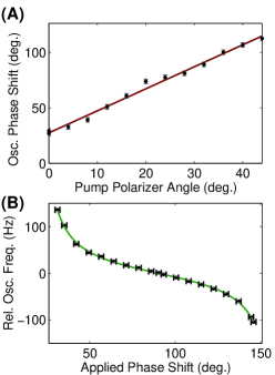
Figure 2: Demonstration of all-optical phase shift. The pump polarization was rotated while the probe polarization was held fixed; for each angular setting a pulse delay (equivalent to an electronic phase shift) was applied to maintain the oscillator on resonance. In (a), this electronic phase shift is plotted against the polarizer angle. The straight-line fit gives a slope of $1.98\pm 0.06$, in good agreement with the expected value of $2$ (see text). In (b), the oscillator frequency as a function of phase shift is plotted. The curve agrees well with the expected form of Eq. (1), although the vertical asymptotes of the tangent fit (solid line) do not occur at $0^{\circ}$ and $180^{\circ}$, probably resulting from a small ($\sim 0.1\%$) residual contribution of scattered pump light to the optical rotation signal. The solid line is a fit to a tangent function. For phase shifts approaching $0^{\circ}$ or $180^{\circ}$, the gain becomes insufficient to sustain self-oscillation.

IV Optical Phase Shift

To emphasize the advantages of the two-beam arrangement for the optical adjustment of the phase shift, we note that optical pumping by linearly polarized light favors the preparation of a state whose alignment symmetry axis is parallel to the pump polarization. At the center of the NMOR resonance, therefore, where there is no phase lag between pumping and precession, the precessing axis of atomic alignment is parallel to the pump polarization at the moment of maximal optical pumping in the limit of short pump pulses. Consequently, if the probe polarization is parallel to the pump polarization, the probe polarization rotation signal will pass through zero at the same moment, so that this optical rotation signal is $90^{\circ}$ out of phase with the pump modulation, as seen in Eq. (1). Thus the rotation signal must be shifted by $-90^{\circ}$ before being fed back as pump modulation in order for coherent buildup at the central resonant frequency to occur. Deviations from this phase shift will result in oscillation away from line center, in such a way as to maintain zero total phase around the loop, so long as the magnitude of the gain is sufficient to sustain oscillation at the shifted frequency. As a result, precise control over this phase shift as a function of frequency is required to avoid (or compensate for) systematic deviations of the oscillation frequency from $2\omega_{L}$ as a function of magnetic field. Analog filter networks capable of generating accurate and stable $90^{\circ}$ phase shifts over a broad range of frequencies are difficult to construct. Digital phase shifters, although feasible, add complexity and power consumption and risk degradation of performance.

The use of separate pump and probe beams offers a natural and all-optical means of shifting the relative phase between modulation and optical rotation. Indeed, since the rotation of the probe polarization is determined by the angle of the incident polarization with respect to the axis of atomic alignment, which itself rotates uniformly in time, a fixed rotation of the incoming probe polarization is equivalent to a translation in time of the output signal, i.e., a phase shift. Since this phase shift is purely geometrical, it has no frequency dependence, and possesses the long-term stability of the mechanical mounting of the polarizers.

To demonstrate the optical phase shift of the polarization-rotation signal, a measurement of the phase shift of the signal as a function of the pump polarizer angle was performed in the open-loop configuration, i.e., with an external frequency source modulating the pump power and with no feedback of the optical-rotation signal. The resulting curve reveals the expected linear dependence, as shown in Fig. 2(a). The observed slope is consistent with the value of $2$ expected from the fact that the optical-rotation signal undergoes two cycles as the atomic alignment rotates by $360^{\circ}$. The effects of a phase shift in the feedback network on the oscillation frequency of the self-oscillating, closed-loop magnetometer are shown in Fig. 2(b). As expected, the magnetometer adjusts its oscillation frequency so that the phase shift of the NMOR resonance cancels that of the feedback network. Since the phase shift of the NMOR resonance is an arctangent function of the detuning from resonance (similar to a damped harmonic oscillator), this results in a change in oscillation frequency which is proportional to the tangent of the applied phase shift, as seen in Fig. 2(b).

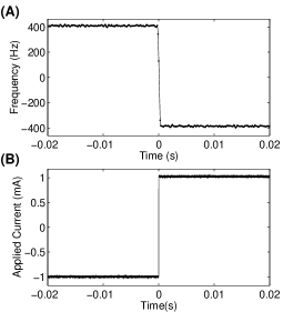
Figure 3: Response of the magnetometer to a $570\,\mu{\rm G}$ step in magnetic field, in the presence of an over-all bias field of $\sim 14\,$mG. This step is thus large compared to the resonance line width, but small compared to the bias field. The self-oscillation waveform was recorded on a digital storage oscilloscope and subsequently fit to a sinusoid in overlapping time windows $500\,\mu{\rm s}$ long, spaced by $125\,\mu{\rm s}$. The resulting frequency is shown in part (a). In part (b), an oscilloscope trace of the bias current proportional to the field step is shown.

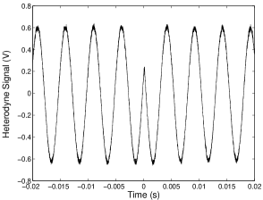
Figure 4: Heterodyne measurement of magnetometer response to a field step. Shown here is the self-oscillating rotation signal mixed down to low frequency by a lock-in amplifier with its reference set to approximately twice the Larmor frequency. This heterodyned signal is shown for a period of approximately $40\,{\rm ms}$ during which a sudden change of $\approx 250\,\mu{\rm G}$ is made to the bias magnetic field. The local oscillator is set midway between the two oscillation frequencies, so that the heterodyne signal appears to reverse itself in time.

V Sinusoidal Output Signal

In most past NMOR experiments, modulation was applied from a stable reference oscillator, and the rotation signal was demodulated by a lock-in amplifier at this reference frequency (or one of its harmonics). On the basis of the lock-in output, the reference frequency could be updated at a rate governed by the lock-in time constant, in order to maintain the resonance condition in a slowly changing magnetic field. By contrast, in the self-oscillating scheme, the measured rotation signal is fed back to the modulation input in place of the reference frequency, as shown in Fig. 1. In order to reproduce self-consistently the effects of an external modulation, this signal must in general be phase shifted and filtered so that it closely resembles the original reference frequency, as in the work of Ref. schwindt2005 .

Indeed, if the probe is frequency- or amplitude-modulated, as is the case for a single-beam experiment, then the observed rotation signal will be the product of the rotation signal that would be observed with an unmodulated probe and a function which describes the modulation. In the case of frequency modulation, for example, the observed rotation signal for an isolated line, Doppler broadened to a width $\Delta\nu_{\rm Doppler}$, would be approximately

$$\phi_{FM}(t)\approx\phi_{un.}(t)e^{{-(\delta_{0}-A\cos 2\pi\nu_{\rm mod}t)^{2}/\Delta\nu_{\rm Doppler}^{2}}},$$

where $\phi_{un.}$ is the rotation that would be observed by an unmodulated probe passing through the same sample, $\delta_{0}$ is the mean detuning of the laser from resonance, $A$ the modulation amplitude, and $\nu_{\rm mod}$ the modulation frequency. Similarly, in the case of pulsed amplitude modulation, the multiplicative modulation function would take the form of a pulse train at the modulation frequency. Since the atomic alignment is described by a rank 2 spherical tensor, and the corresponding spin probability distribution is two-fold symmetric (see, for example, Ref. Rochester2001 ), the unmodulated rotation signal is to good approximation sinusoidal at twice the Larmor frequency, $2\omega_{L}$. (Note that this argument neglects the effects of alignment-to-orientation conversion Bucker_AOC_2000 , which becomes important at relatively large light powers.) The over-all rotation signal detected by a modulated probe, however, is in general highly non-sinusoidal. For stable and reproducible operation, such a signal would almost certainly require filtering, which generically introduces undesirable phase shifts. In contrast, the use of an unmodulated probe avoids this complication altogether. The detected rotation signal is a near-perfect sinusoid (measurements indicate that the higher harmonics are down by more than $50\,$dB). Such a signal requires only amplification to make it mimic the reference oscillator.

VI High-speed Response

In order to assess the bandwidth of the magnetometer, the response to rapid changes in magnetic field was investigated by applying a small modulation to the bias magnetic field. In one measurement, a slow square-wave modulation was superimposed on the bias field via a separate Helmholtz coil inside the magnetic shield. The self-oscillation signal was then recorded on an oscilloscope and fit in each $500\,\mu{\rm s}$ window to a sinusoid, with the results shown in Fig. 3. Tracking of the field step is quasi-instantaneous, without apparent overshoot or ringing. The magnetometer response was also monitored by heterodyning the oscillation frequency with a fixed reference frequency on a lock-in amplifier, with the lock-in time constant set to approximately the oscillation period ($\approx 50\,\mu{\rm s}$) to remove the sum-frequency component. The resulting low-frequency beat signal, which displayed large fractional frequency modulation, was also digitized and recorded on an oscilloscope. Inspection of the waveforms so obtained revealed the same sudden shift in the oscillation frequency as the magnetic field toggled between values (see Fig. 4). In a related experiment, the bias field received a small sinusoidal modulation, and the power spectrum of the self-oscillation waveform was observed on a spectrum analyzer. The sidebands were observed, offset from the oscillation (carrier) frequency by an amount equal to this bias-modulation frequency; their relative power was equal to that expected if the oscillator tracked the changing magnetic field with no delay or diminution of amplitude out to a bias-modulation frequency of at least $1\,{\rm kHz}$.

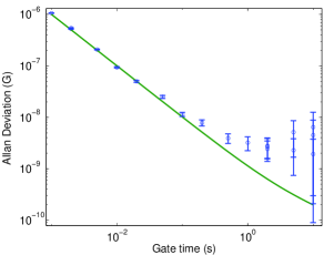
Figure 5: Allan deviation of magnetometer as obtained from counter. The solid line indicates the calculated sensitivity given by Eq. (9), showing good agreement for short measurement times.

VII Comparison with Calculated Sensitivity

To evaluate the performance of the magnetometer, it is useful to calculate the performance that is expected from measurable system parameters as a function of the measurement time. The self-oscillating magnetometer is similar in many respects to a maser, as was first pointed out in Ref. Bloom1962 ; a treatment of noise in the hydrogen maser system is given in Ref. Vanier . The read-out device envisioned here is a frequency counter that measures to high precision the elapsed time between two zero-crossings of the rotation signal and reports a frequency which is the integer number of zero-crossings divided by this time.

Noise in the magnetometer readings comes from several sources. These include fundamental noise, such as atomic and photon shot noise, as well as technical noise from electronics. Fluctuations in the measured field also appear as noise, but do not represent a failing of the magnetometer. For a transmitted probe beam power of $P=2.5\,\mu{\rm W}$, the optical shot noise for an ideal polarimeter, given in terms of the photon energy $E_{\rm ph}$ by $\sqrt{2E_{\rm ph}P}$, is $1.1\,{\rm pW}/\sqrt{\,{\rm Hz}}$ or $0.55\,{\rm pA}/\sqrt{\,{\rm Hz}}$ in terms of the differential photocurrent noise. Atomic shot noise is expected to contribute a comparable noise level for an optimized magnetometer Auzinsh2004 . Observed amplifier noise is somewhat larger than the photon shot-noise level, or $0.8\,{\rm pA}/\sqrt{\,{\rm Hz}}$, and can be considered as white noise over the relevant bandwidth ($\apprle 5\,{\rm kHz}$) around the operation frequency of $20\,{\rm kHz}$. For comparison, the optimized self-oscillation signal amplitude, hereafter denoted $I_{0}$, is $14\,\rm{nA}$.

Noise contributes to the uncertainty in the measurement of the self-oscillation frequency in two essential ways. First, it imparts random shifts to the times of the signal zero-crossings, resulting in jitter of the frequency-counter trigger times and of the corresponding reported frequency. Second, noise within the NMOR resonance bandwidth drives the atomic resonance, resulting in random drifts of the phase of oscillation and limiting the precision of the frequency measurement. We will consider each of these in turn, both for the observed noise level and for the photon-shot-noise limit.

Jitter of the counter triggers can be derived from a photocurrent difference signal

$$I(t)=I_{0}\sin(2\pi\nu_{0}t)+\Delta I(t).$$

Here, $\Delta I(t)$ is additive noise, e.g., photon shot noise or amplifier noise, referred to the amplifier input, i.e., expressed as a photocurrent, and $\nu_{0}$ is the mean self-oscillation frequency. Provided that $\Delta I(t)$ is small, the zero-crossings of this signal experience a r.m.s. fluctuation

$$\Delta t_{\rm zero}=\frac{\Delta I_{\rm rms}}{2\pi\nu_{0}I_{0}}.$$ (2)

If the open-loop noise spectrum is approximately white in the vicinity of $\nu_{0}$, then the r.m.s. current is simply given by $\Delta I_{\rm rms}=\sqrt{2S_{I}\nu_{\rm max}}$, where $2\nu_{\rm max}$ is the bandwidth around $\nu_{0}$ defined, for instance, by a filter in the loop, and $S_{I}$ is the single-sided current power spectral density, with units of ${\rm A}_{\rm rms}^{2}/\,{\rm Hz}$. The r.m.s. deviation of the interval between two zero crossings $\Delta t_{\rm meas}$ is $\sqrt{2}$ times the deviation of each separately, so that the total uncertainty in the frequency reading of the magnetometer due to trigger jitter is

$$\Delta\nu_{\rm jitt} = \nu_{0}{\Delta t_{\rm meas}}/{T}$$ (3)

$$= \frac{(S_{I}\nu_{\rm max})^{1/2}}{\pi TI_{0}},$$

where $T$ is the measurement duration.

The second effect of noise on the operation of the magnetometer is due to the feedback network that produces self-oscillation. As shown below, noise that is within the linewidth of the NMOR resonance mimics a fluctuating phase shift in the self-oscillating loop. This phase shift produces random fluctuations in the oscillation frequency, inducing diffusion of the over-all phase of oscillation. For notational simplicity, let us first consider a single frequency component of the noise at a frequency $\nu_{0}+\nu_{\rm off}$, where $\nu_{\rm off}$ is referred to as the offset frequency. For an open-loop magnetometer, i.e., with modulation supplied by an external frequency source tuned to the NMOR resonance and no feedback of the optical rotation signal, the resulting photocurrent difference signal would be

$$I(t) = I_{0}\sin(2\pi\nu_{0}t)+\epsilon\sin(2\pi(\nu_{0}+\nu_{\rm off})t)$$ (4)

$$\approx I_{0}\sin\left(2\pi\nu_{0}t+\frac{\epsilon}{I_{0}}\sin(2\pi\nu_{\rm off}t)\right),$$

where $\epsilon$ is taken to be small, and a term contributing only to amplitude modulation of the signal has been neglected. The phase of the noise component has been chosen arbitrarily but plays no role in what follows. Equation (4) shows that the effect of this noise component is to modulate the phase of the open-loop signal with an amplitude $\epsilon/I_{0}$ at frequency $\nu_{\rm off}$. When the self-oscillating loop is closed, the oscillation responds to this noise-induced phase shift by shifting the frequency of oscillation in such a way as to keep the net phase shift around the loop zero. The magnitude of the resulting frequency modulation of the self-oscillating signal is readily calculated from Eq. (1), which may be approximated over the central portion of the resonance as linear, i.e., $\nu_{\rm off}\approx\gamma\phi/4\pi$, so that the amplitude of the induced frequency modulation is $\gamma\epsilon/4\pi I_{0}$. The resulting self-oscillation signal is

$$I(t) = I_{0}\sin\int_{0}^{t}{\rm d}t^{\prime}\left(2\pi\nu_{0}+\frac{\gamma\epsilon}{2I_{0}}\sin 2\pi\nu_{\rm off}t^{\prime}\right)$$ (5)

$$= I_{0}\sin\left(2\pi\nu_{0}t-\frac{\gamma\epsilon}{4\pi I_{0}\nu_{\rm off}}\cos 2\pi\nu_{\rm off}t\right),$$

where the global phase of oscillation has been taken to be zero at $t=0$. In analogy to Eq. (2), the r.m.s. deviation of a zero-crossing of this signal at a randomly chosen time is

$$\Delta t_{\rm zero}=\frac{\gamma\epsilon}{4\pi I_{0}\nu_{\rm off}}\frac{1}{2\pi\nu_{0}\sqrt{2}},$$

and the corresponding frequency uncertainty from phase diffusion is

$$\Delta\nu_{\rm diff}=\frac{\gamma\epsilon}{4\pi I_{0}\nu_{\rm off}}\frac{1}{2\pi T}.$$ (6)

Although this expression diverges for $\nu_{\rm off}\rightarrow 0$, in reality a measurement lasting a time $T$ imposes an effective low-frequency cut-off of $\approx 1/T$. To take into account the fact that the noise contains many incoherent spectral components, rather than a single monochromatic component, one must add these components in quadrature. Thus, it is sufficient to replace the original mean square current modulation $\epsilon^{2}/2$ at frequency $\nu_{\rm off}$, by the photocurrent noise power $S_{I}{\rm d}\nu_{\rm off}$ in a range ${\rm d}\nu_{\rm off}$ around frequency $\nu_{0}+\nu_{\rm off}$, and integrate the result over the appropriate range of frequency. For a measurement time $T$, the minimum resolvable frequency is $\approx 1/T$. The maximum frequency at which this noise-induced frequency shift occurs is $\approx\gamma/2$, but for times $T\apprge 2/\gamma$, which in practice include all times for which this type of noise is dominant, we may reasonably approximate the range of integration as extending to infinity. Note that noise on either side of $\nu_{0}$ contributes equally, so that the total integral is twice the integral evaluated on the positive side only. Thus Eq. (6) must be modified to

$$\Delta\nu_{\rm diff} \approx \frac{\gamma\sqrt{2}}{8\pi^{2}I_{0}T}\left|2\int_{1/T}^{\infty}{\rm d}\nu_{\rm off}\frac{S_{I}(\nu_{0}+\nu_{\rm off})}{\nu_{\rm off}^{2}}\right|^{1/2}$$ (7)

$$\approx \frac{\gamma}{4\pi^{2}\sqrt{T}}\frac{S_{I}^{1/2}}{I_{0}}.$$

The photocurrent noise spectrum $S_{I}$ has been assumed white over the range of integration in evaluating the integral.

This intra-resonance noise can also be understood in terms of phase diffusion Lax1967 . Indeed, although the frequency of the oscillation is stabilized to twice the Larmor frequency in the self-oscillating scheme, the global phase of oscillation experiences no feedback or restoring force, and is thus subject to an effective Brownian motion or diffusion, where shot noise or amplifier noise provides a stochastic driving force. In this picture, the phase undergoes a random walk, with a step size given by the r.m.s. noise within the resonance and a time step given by $\sim 1/\gamma$. Explicitly, the total phase noise within the resonance yields a step size $\Delta\phi_{\rm step}\approx(S_{I}^{1/2}/I_{0})\sqrt{\gamma/2\pi}$. After a time $T$ the number of steps is approximately $N_{\rm steps}=\gamma T$, so that the total frequency uncertainty given by

$$\Delta\nu_{\rm diff} \approx \frac{\Delta\phi_{\rm step}}{2\pi T}\sqrt{N_{\rm steps}}$$ (8)

$$\approx \frac{1}{(2\pi)^{3/2}}\frac{S_{I}^{1/2}}{I_{0}}\frac{\gamma}{T^{1/2}},$$

which agrees up to a numerical factor with Eq. (7)

Numerically, for the experimental parameters discussed above, we have $S_{I}^{1/2}/I_{0}=6\times 10^{-5}\,\,{\rm Hz}^{-1/2}$, $\gamma=2\pi\times 80\,{\rm Hz}$, and $\nu_{\rm max}=5\,{\rm kHz}$ (the measured bandwidth of an LC filter in the loop), so that Eqs. (3) and (7) imply a magnetic-field sensitivity limit of

$$\Delta B=\left\{\left(\frac{1.0\,{\rm nG}}{T/1\,{\rm s}}\right)^{2}+\left(\frac{0.54\,{\rm nG}}{\sqrt{{T/1\,{\rm s}}}}\right)^{2}\right\}^{1/2}.$$ (9)

Equation (9) is in good agreement with the measured data for times below $\sim 0.1\,{\rm s}$, as shown in Fig. 5, while above $\sim 0.1\,{\rm s}$ measurements fall short of calculated performance, as discussed below.

It should be noted that the initial $1/T$ dependence of the sensitivity is non-optimal. If information about the phase during the entire duration $T$ were retained and the frequency extracted (e.g. by least-squares fitting), then this dependence could be improved by an additional factor of approximately $\sqrt{T_{\rm samp}/T}$, where $T_{\rm samp}$ is a sampling time, provided $1/T_{\rm samp}$ is smaller than the noise bandwidth, e.g., the filter frequency $\nu_{\rm max}$. The improved scaling would then be $\propto T^{-3/2}$. For measurement times $\apprge 1\,{\rm s}$, however, this is not a limiting factor sufficient to outweigh the frequency counter’s considerable convenience. The result of Eq. (9) is within a factor of two of the optical-shot-noise limit for the same system parameters, although with a quieter photodiode amplifier, further optimization of light powers, detunings, and ⁸⁷Rb density should permit operation with narrower resonance lines and considerable consequent improvement.

For measurement times $T$ exceeding $\sim 0.1\,{\rm s}$, additional sources of noise not present in the model discussed so far become dominant, obscuring the phase-diffusion noise. In order to distinguish between magnetic and instrumental noise, we have measured fluctuations of ambient magnetic fields with a fluxgate magnetometer external to the shields at approximately $20\,\mu{\rm G}/\sqrt{\,{\rm Hz}}$ above a $1/f$ corner frequency of approximately $0.3\,{\rm Hz}$. With a measured shielding factor of $3\times 10^{5}$, this implies a negligibly small white magnetic-field noise of around $70\,{\rm pG}/\sqrt{\,{\rm Hz}}$ at the vapor cell. The expected average noise on the supplied bias field inside the shield is better than $6\,{\rm nG}/\sqrt{\,{\rm Hz}}$ between $0.1\,{\rm Hz}$ and $100\,{\rm Hz}$. This value is of the same order of magnitude as the observed Allan deviation floor, although direct and reliable measurements of this bias current have not been achieved. Noise on the bias-field current could be distinguished from other sources by use of a magnetic gradiometer (see, for example, a description of a gradiometer based on a pair of FM NMOR sensors in Ref. xu2006 ), though the small size of our magnetic shield has so far precluded such a measurement.

Other noise sources include sensitivities of the oscillation frequency to laser powers and detuning. A sensitivity to pump or probe power arises, for instance, when the feedback-network phase shift deviates from the value which produces maximal oscillation amplitude. Since the NMOR phase shift depends on the resonance line width as in Eq. (1), while the line width depends on optical power through the effect of power-broadening, changes in pump or probe power produce changes in phase shift and corresponding deviations of the self-oscillation frequency. This effect vanishes to first order precisely on the NMOR resonance; additional mechanisms for translating power and detuning fluctuations into oscillation-frequency fluctuations are currently being investigated.

VIII Conclusion

We have demonstrated a self-oscillating two-beam magnetometer based on nonlinear magneto-optical rotation and shown that the independent adjustment of pump and probe polarizations provides a powerful and frequency-independent means of supplying the phase shift necessary for self-oscillation. Moreover, the use of an unmodulated probe eliminates the necessity of elaborate filtering procedures, producing instead a clean sine wave suitable for feeding back as the self-modulation signal. The resulting device possesses a high bandwidth and a measured sensitivity of $3\,{\rm nG}$ at $1\,{\rm s}$. Considerable improvement, approaching the fundamental atomic and optical shot-noise limit of $\apprle 30\,{\rm pG}$ in $1\,{\rm s}$ measurement time for a $\sim 6\,{\rm cm}^{3}$ cell, is expected through a more thorough control of light-power-dependent, laser-frequency-dependent, and electronic phase shifts, as well as through re-optimization using a quieter amplifier. The fundamental constituents of this magnetometer are small and lightweight, lending themselves well to designs for the field and for space. Operation in the geomagnetic range of fields has been achieved. In future work, the robustness of the magnetometer in an unshielded environment and an arbitrarily directed geomagnetic field will be investigated. Performance in the presence of splitting of the resonance line by the quadratic Zeeman shift will also be evaluated.

The authors acknowledge discussions with E. B. Alexandrov, S. M. Rochester and J. Kitching and contributions of V. V. Yashchuk and J. E. Stalnaker to the design and construction of the magnetic shields, coils, and the vapor-cell heating system. This work is supported by DOD MURI grant # N-00014-05-1-0406, by an ONR STTR grant through Southwest Sciences, Inc., and by an SSL Technology Development Grant.

References

- (1) I. K. Kominis, T. W. Kornack, J. C. Allred, and M. V. Romalis, Nature (London)422, 596 (2003).
- (2) A. Nagel, L. Graf, A. Naumov, E. Mariotti, V. Biancalana, D. Meschede, and R. Wynands, Europhys. Lett. 44, 31 (1998).
- (3) C. Affolderbach, M. Stähler, S. Knappe, and R. Wynands, Appl. Phys. B 75, 605 (2002).
- (4) G. Bison, R. Wynands, and A. Weis, Appl. Phys. B 76, 325 (2003).
- (5) H. Xia, A. B. Baranga, D. Hoffman, and M. V. Romalis, To be published. (2006).
- (6) S. A. Murthy, J. D. Krause, Z. L. Li, and L. R. Hunter, Phys. Rev. Lett. 63, 965 (1989).
- (7) C. J. Berglund, L. R. Hunter, J. D. Krause, E. O. Prigge, M. S. Ronfeldt, and S. K. Lamoreaux, Phys. Rev. Lett. 75, 1879 (1995).
- (8) A. N. Youdin, D. K. Jr., K. Jagannathan, L. R. Hunter, and S. K. Lamoreaux, Phys. Rev. Lett. 77, 2170 (1996).
- (9) M. V. Romalis, W. C. Griffith, J. P. Jacobs, and E. N. Fortson, Phys. Rev. Lett. 86, 2505 (2001).
- (10) J. M. Amini and H. Gould, Phys. Rev. Lett. 91, 153001 (2003).
- (11) S. Groeger, G. Bison, J.-L. Schenker, R. Wynands, and A. Weis, Eur. Phys. Jour. D 38, 239 (2006).
- (12) P. D. D. Schwindt, S. Knappe, V. Shah, L. Hollberg, J. Kitching, L.-A. Liew, and J. Moreland, Appl. Phys. Lett. 85, 6409 (2004).
- (13) D. Budker, D. F. Kimball, S. M. Rochester, V. V. Yashchuk, and M. Zolotorev, Phys. Rev. A62, 043403 (2000).
- (14) V. Acosta, M. P. Ledbetter, S. M. Rochester, D. Budker, D. F. Jackson Kimball, D. C. Hovde, W. Gawlik, S. Pustelny, J. Zachorowski, and V. V. Yashchuk, Phys. Rev. A73, 053404 (2006).
- (15) M. H. Acuna, Rev. Sci. Inst. 73, 3717 (2002).
- (16) A. L. Bloom, Appl. Opt. 1, 61 (1962).
- (17) P. D. D. Schwindt, L. Hollberg, and J. Kitching, Rev. Sci. Inst. 76, 126103 (2005).
- (18) D. Budker, V. Yashchuk, and M. Zolotorev, Phys. Rev. Lett. 81, 5788 (1998).
- (19) D. Budker, D. F. Kimball, V. V. Yashchuk, and M. Zolotorev, Phys. Rev. A65, 055403 (2002).
- (20) W. Gawlik, L. Krzemien, S. Pustelny, D. Sangla, J. Zachorowski, M. Graf, A. O. Sushkov, and D. Budker, Appl. Phys. Lett. 88, 131108 (2006).
- (21) K. L. Corwin, Z.-T. Lu, C. F. Hand, R. J. Epstein, and C. E. Wieman, Appl. Opt. 37, 3295 (1998).
- (22) V. V. Yashchuk, D. Budker, and J. R. Davis, Rev. Sci. Inst. 71, 341 (2000).
- (23) S. M. Rochester and D. Budker, Am. J. Phys. 69, 450 (2001).
- (24) D. Budker, D. F. Kimball, S. M. Rochester, and V. V. Yashchuk, Phys. Rev. Lett. 85, 2088 (2000).
- (25) J. Vanier and C. Audoin, The Quantum Physics of Atomic Frequency Standards (Adam Hilger, Philadelphia, 1989), Vol. 2.
- (26) M. Auzinsh, D. Budker, D. F. Kimball, S. M. Rochester, J. E. Stalnaker, A. O. Sushkov, and V. V. Yashchuk, Phys. Rev. Lett. 93, 173002 (2004).
- (27) M. Lax, Phys. Rev. 160, 290 (1967).
- (28) S. Xu, S. M. Rochester, V. V. Yashchuk, M. H. Donaldson, and D. Budker, Rev. Sci. Inst. 77, 083106 (2006).