On chemisorption of polymers to solid surfaces

Abstract. The irreversible adsorption of polymers to a two-dimensional solid surface is studied. An operator formalism is introduced for chemisorption from a polydisperse solution of polymers which transforms the analysis of the adsorption process to a set of combinatorial problems on a two-dimensional lattice. The time evolution of the number of polymers attached and the surface area covered are calculated via a series expansion. The dependence of the final coverage on the parameters of the model (i.e. the parameters of the distribution of polymer lengths in the solution) is studied. Various methods for accelerating the convergence of the resulting infinite series are considered. To demonstrate the accuracy of the truncated series approach, the series expansion results are compared with the results of stochastic simulation.

1 Introduction

The adsorption of polymers to solid surfaces has wide technological and medical applications [14, 8]. In this paper, we study chemisorption, i.e. the situation where covalent surface-polymer bonds develop and adsorption is effectively irreversible on the experimental time scale [13]. Chemisorbing polymers have one or more reactive (binding) groups along the polymer chain which can react with binding sites on the surface. Polymers with one reactive group at the end of the chain are called semitelechelic. A schematic diagram of the adsorption of a semitelechelic polymer is shown in Figure 1(a) where the binding sites are arranged into a rectangular mesh on the surface. An important parameter of the chemisorption process is the density of binding sites, or equivalently, the average distance between neigbouring sites, which is denoted by $h$ in Figure 1(a). Denoting the hydrodynamic radius of the polymer by $R$, we can distinguish three different scenarios. If $h\ll R$, then the polymer layer created by chemisorption of the semitelechelic polymer will be a polymer brush after sufficiently long time [11, 9, 21]. In this case, one can simply assume that a polymer can attach anywhere on the surface for modelling purposes. In particular, one can use continuum random sequential adsorption to model the process [3]. The other extreme case is $h\gg R$ where the final layer contains one attached polymer at each binding site. No steric shielding needs to be considered when modelling the process and the dynamics of adsorption is trivial from the mathematical point of view. The last important case is when $h\sim R$. This is the regime studied in this paper.

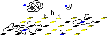
(a)        (b)

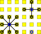
Figure 1: (a) A schematic diagram of the chemisorption of the semitelechelic polymer. (b) Situation from (a) transformed into two-dimensional lattice setting.

Chemisorption is often modelled as a random sequential adsorption (RSA) [4, 16]. In a previous paper [3] we studied one-dimensional models of random sequential (irreversible) adsorption. Our motivation was to understand the essential processes involved in pharmacological applications such as the polymer coating of viruses [8]. The classical RSA model [4] was generalized to study the effects of polydispersity of polymers in solution, of partial overlapping of the adsorbed polymers, and the influence of reactions with the solvent on the adsorption process. Working in one dimension, we derived an integro-differential evolution equation for the adsorption process and we studied the asymptotic behaviour of the quantities of interest, namely the surface area covered and the number of molecules attached to the surface. We also presented applications of equation-free dynamics renormalization tools [10] to study the asymptotically self-similar behaviour of the adsorption process. In [3] we used a continuum RSA model. The underlying assumption was that the polymer can effectively bind anywhere on the surface, i.e. we worked in the regime $h\ll R.$ In reality, the reactive groups on the polymer can react only with the corresponding binding sites on the surface, which are primary amino-groups in the virus coating problem. Rough estimates from molecular models suggest that the average distance between primary amino-groups in the virus capsid is about a nanometre [7]. However, it is difficult to guess which of the amino-groups in the capsid are available for the reaction with the polymer, i.e. are accessible for polymers from solution. In particular, both the regimes $h\ll R$ and $h\sim R$ can be justified in the virus coating problem. Other chemisorbing systems [14, 4] can be also used to motivate investigation of the borderline case $h\sim R$.

Assuming $h\sim R$, we have to take the discrete nature of the binding sites into account. This means that lattice RSA modelling is more appropriate than continuum RSA modelling. In this paper we assume for simplicity that the binding sites lie on a rectangular mesh (see Figure 1), with mesh points a distance $h$ apart. We choose $h=1$ without loss of generality in what follows. Any polymer covers the binding site to which it is attached. Moreover, longer polymers also effectively cover neighbouring binding sites, as illustrated in Figure 1(a). More precisely, an attached semitelechelic polymer covers a circle of a certain radius $r$ which is centered at the binding site (meshpoint $(i,j)$). If $r<1$, then the polymer effectively covers only the corresponding binding site $(i,j)$. If $1\leq r<\sqrt{2}$, then the polymer covers a small “cross” ${\cal X}_{i,j}$ where we define

$${\cal X}_{i,j}=\big{\{}(i,j),(i+1,j),(i-1,j),(i,j-1),(i,j+1)\big{\}}.$$ (1.1)

We call set of mesh points ${\cal X}_{i,j}$ the cross (or cross-polymer) centered at $(i,j)$. If $\sqrt{2}\leq r<2$, then the polymer covers a small “square” ${\cal S}_{i,j}$ defined by

$${\cal S}_{i,j} = \big{\{}(i,j),(i+1,j),(i-1,j),(i,j-1),(i,j+1),$$ (1.2)

$$\;\;(i+1,j+1),(i+1,j-1),(i-1,j+1),(i-1,j-1)\big{\}}.$$

We call set of mesh points ${\cal S}_{i,j}$ the square (or square-polymer) centered at $(i,j)$. If $2<r$, then the polymer covers at least 13 binding sites. To simplify the combinatorial complexity of the problem, we restrict our consideration to the case $r<2$. In this case, we can formulate the chemisorption of polymers in terms of adsorption of points, crosses and squares to the two-dimensional lattice (see Figure 1(b)). We denote by $\alpha$ the fraction of polymers in the solution for which $1\leq r<\sqrt{2}$, so that $\alpha$ is the probability that a randomly chosen polymer in solution will adsorb as a cross. Similarly, we denote $\beta$ the fraction of polymers in the solution for which $\sqrt{2}\leq r<2$ so that $\beta$ is the probability that a randomly chosen polymer in solution will adsorb as a square. In particular, we must have $0\leq\alpha+\beta\leq 1$ where $1-\alpha-\beta$ is the probability that a randomly chosen polymer in solution will adsorb as a point. We work with an $M\times M$ mesh with periodic boundary conditions. Then our two-dimensional polydisperse random sequential adsorption (pRSA) algorithm can be stated as follows.

pRSA algorithm: We consider the adsorption of points $\{(i,j)\}$, crosses ${\cal X}_{i,j}$ and squares ${\cal S}_{i,j}$ to the two-dimensional rectangular $M\times M$ mesh. At each time step, we choose randomly a point $(i,j)$ in the mesh. If the selected mesh point $(i,j)$ is covered (occupied) by a point/cross/square already placed, the adsorption is rejected. If the mesh point $(i,j)$ is vacant, then it is marked as occupied. Moreover, with probability $\alpha$ (resp. $\beta$), all mesh points in the set ${\cal X}_{i,j}$ (resp. ${\cal S}_{i,j}$) are marked as occupied.

To simulate pRSA algorithm, we have to generate three random numbers at each time step. The first two of them are used for random selection of the lattice point where the reactive group of the adsorbed polymer is attempted to bind. The third random number $r_{n}$, uniformly distributed in interval $[0,1]$, is used to determine the length of the adsorbed polymer. If $r_{n}\in[0,\alpha)$, then the cross polymer is placed. If $r_{n}\in[\alpha,\alpha+\beta)$, then the square-polymer is chosen. If $r_{n}\in[\alpha+\beta,1]$, then the point-polymer is adsorbed. An illustrative numerical simulation of pRSA algorithm for $\alpha=0.8$ and $\beta=0.1$

​​​​​​​​​​​​​​​​​​​​

​​​​​​​​​​​​​​​​​​​​

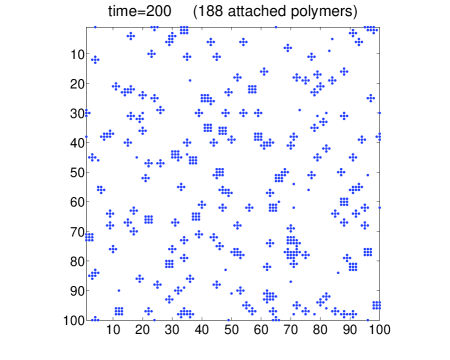
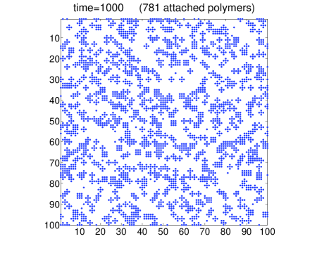
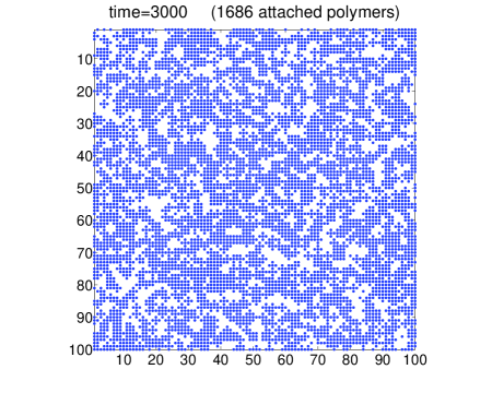
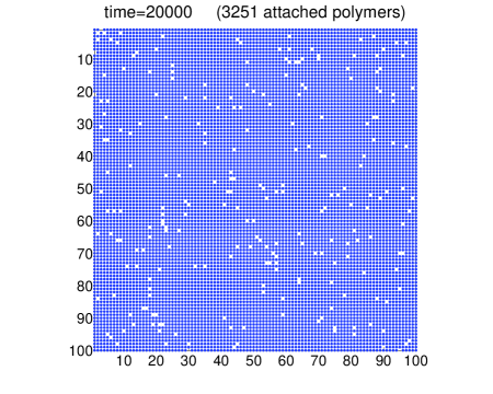
Figure 2: One realization of pRSA algorithm for $\alpha=0.8$ and $\beta=0.1$. The covered mesh points of the rectangular $100\times 100$ mesh are shown at different times.

is shown in Figure 2. We start with an empty rectangular $100\times 100$ mesh, i.e. $M=100.$ The mesh points covered by polymers are plotted at different times.

Let us note that pRSA algorithm requires that the position $(i,j)$ of the center of the adsorbed cross ${\cal X}_{i,j}$ (resp. square ${\cal S}_{i,j}$) is vacant. On the other hand, the “tails” of crosses/squares can overlap. Here, the center of the cross (resp. square) describes the reactive group which is covalently bound to the surface. The remaining four (resp. eight) points of the cross (resp. square) describe the polymer tails which sterically shield the neighbourhood of the adsorbed polymer. In our algorithm, binding of a larger polymer prevents binding (of the center) of another polymer in the neighbourhood of the center of the polymer already adsorbed. On the other hand, the “wiggling tails” of polymers can overlap.

As in [3] there are two important quantities of interest: the number of covered mesh points $A(t)$ and the number $N(t)$ of polymers which are attached to the surface at time $t$. To understand the behaviour of $A(t)$ and $N(t)$, we introduce in Section 2 an operator formalism which makes it possible to derive a series expansion for $N(t)$. We also derive series for $A(t)$ and for numbers of point-polymers, cross-polymers and square-polymers adsorbed on the surface at time $t$. The operator formalism transforms the random sequential adsorption process into a set of combinatorial problems on the lattice. In some special cases, one can further simplify the resulting lattice combinatorial problems; we consider these special cases in Section 3. The general problem is studied in Section 4. To illustrate the precision of the derived formulas, we also provide a comparison of the results obtained by series expansion with those obtained by direct stochastic simulation, of particular interest is the time evolution of $A(t)$ and $N(t)$ and the dependence of the final adsorbed polymer layer on the parameters $\alpha$ and $\beta$. We conclude with a discussion in Section 5.

2 Operator formalism

Let us denote by $N(t)$ (resp. $N_{p}(t)$, $N_{c}(t)$ and $N_{s}(t)$) the number of polymers (resp. point-polymers, cross-polymers and square-polymers) which are adsorbed on the surface at time $t$. Then we have

$$N_{p}(t)=(1-\alpha-\beta)N(t),\qquad N_{c}(t)=\alpha N(t),\qquad N_{s}(t)=\beta N(t).$$ (2.1)

Let $A(t)$ (resp. $F(t)$) be the number of covered (resp. vacant) mesh points at time $t$. Since $dN/dt=F/M^{2}$ and $A=M^{2}-F$, we have

$$A(t)=M^{2}\left(1-\frac{\mbox{d}N}{\mbox{d}t}(t)\right).$$ (2.2)

Let us define

$$N^{\infty}=\lim_{t\to\infty}N(t),\quad N_{p}^{\infty}=\lim_{t\to\infty}N_{p}(t),\quad N_{c}^{\infty}=\lim_{t\to\infty}N_{c}(t),\quad N_{s}^{\infty}=\lim_{t\to\infty}N_{s}(t).$$ (2.3)

Then (2.1) implies

$$N_{p}^{\infty}=(1-\alpha-\beta)N^{\infty},\qquad N_{c}^{\infty}=\alpha N^{\infty},\qquad N_{s}^{\infty}=\beta N^{\infty}.$$ (2.4)

Hence, the saturating values $N_{p}^{\infty},$ $N_{c}^{\infty}$ and $N_{s}^{\infty}$ can be computed directly from $N^{\infty}$. Similarly, the time evolution of $A(t)$, $N_{p}(t)$, $N_{c}(t)$ and $N_{s}(t)$ can be obtained from $N(t)$ by (2.1) – (2.2). In this section, we develop an operator formalism framework to obtain the time evolution of $N(t)$ and the limit $N^{\infty}$. Once we get $N(t)$ and $N^{\infty}$, the rest of quantities of interest can be expressed by (2.1), (2.2) and (2.4) and their dependence on the model parameters $\alpha$ and $\beta$ can be also studied.

In [1, 5], an operator formalism was developed for studying the square lattice with nearest-neighbour exclusion. The results can be directly used to find an approximation of $N^{\infty}$ for $\alpha=1$ and $\beta=0$. If $\alpha=1$, then it is sufficient to keep track of the centers of cross-polymers. Each center of a cross-polymer excludes putting another center of a cross-polymer in the nearest neighbourhood of it. Hence, one can reformulate pRSA algorithm for $\alpha=1$ in terms of adsorption of points which excludes the nearest neighbourhood of them. Similarly, one can reformulate the pRSA algorithm as adsorption of points which excludes the nearest and the next nearest neighbourhood of them for $\alpha=0$ and $\beta=1$. However, if $[\alpha,\beta]\not\in\{[0,1],[1,0],[0,0]\}$, then we have a mixture of polymers of different sizes in the solution and the approach of [1, 5] cannot be directly used. In this section we present a generalization of the operator formalism for the case of arbitrary $\alpha$ and $\beta$.

We consider an $M\times M$ lattice (with periodic boundary conditions) to which polymers can adsorb. For each lattice point $(i,j)$, we consider the state function $\nu_{i,j}\in\{0,1,2,3\}.$ Here, $\nu_{i,j}=0$ means that lattice point $(i,j)$ is vacant or occupied by the “wiggling tail” of a cross-polymer/square-polymer (i.e. $\nu_{i,j}=0$ means that lattice point $(i,j)$ is free of centers of polymers/attached reactive groups), $\nu_{i,j}=1$ means that lattice point $(i,j)$ is occupied by the point-polymer, $\nu_{i,j}=2$ means that the lattice point is occupied by the center of the cross-polymer and $\nu_{i,j}=3$ means that the lattice point is occupied by the center of the square-polymer. Denoting

$$|0\rangle=[1,0,0,0]^{T}\!\!,\qquad|1\rangle=[0,1,0,0]^{T}\!\!,\qquad|2\rangle=[0,0,1,0]^{T}\!\!,\qquad|3\rangle=[0,0,0,1]^{T}\!\!,$$

we identify every lattice point with the four-dimensional vector space $\mathbb{R}^{4}$. Namely, the configuration of the $M\times M$ lattice will be expressed as

$$|\{\nu_{i,j}\}\rangle\in\mathop{\bigoplus}_{i,j=1}^{M}\Big{\{}|0\rangle,|1\rangle,|2\rangle,|3\rangle\Big{\}}.$$

The system state is given by

$$|\Psi(t)\rangle=\sum_{\{\nu_{i,j}\}}P(\{\nu_{i,j}\},t)|\{\nu_{i,j}\}\rangle$$ (2.5)

where the sum is taken over all possible configurations $\{\nu_{i,j}\}$ of the lattice and $P(\{\nu_{i,j}\},t)$ is the probability of each configuration. It satisfies the normalization condition

$$\sum_{\{\nu_{i,j}\}}P(\{\nu_{i,j}\},t)=1.$$ (2.6)

For each lattice point, we define cross, square and point annihilation operators

$${\mathbf{A}}=\left(\begin{matrix}0&0&1&0\\ 0&0&0&0\\ 0&0&0&0\\ 0&0&0&0\end{matrix}\right),\qquad{\mathbf{B}}=\left(\begin{matrix}0&0&0&1\\ 0&0&0&0\\ 0&0&0&0\\ 0&0&0&0\end{matrix}\right),\qquad{\mathbf{C}}=\left(\begin{matrix}0&1&0&0\\ 0&0&0&0\\ 0&0&0&0\\ 0&0&0&0\end{matrix}\right).$$ (2.7)

More precisely, operator ${\mathbf{A}}_{i,j}$ (resp. ${\mathbf{B}}_{i,j}$, and ${\mathbf{C}}_{i,j}$) acts as ${\mathbf{A}}$ (resp. ${\mathbf{B}}$, and ${\mathbf{C}}$) on the lattice point $(i,j)$ and as the identity on all other lattice points. We also define creation operator ${\mathbf{A}}_{i,j}^{\dagger}$ (resp. ${\mathbf{B}}_{i,j}^{\dagger}$, and ${\mathbf{C}}_{i,j}^{\dagger}$) as the transpose of operator ${\mathbf{A}}_{i,j}$ (resp. ${\mathbf{B}}_{i,j}$, and ${\mathbf{C}}_{i,j}$). The cross-polymer number operator (resp. square-polymer number operator, and point-polymer number operator) is defined as ${\mathbf{N}}^{c}_{i,j}={\mathbf{A}}_{i,j}^{\dagger}{\mathbf{A}}_{i,j}$ (resp. ${\mathbf{N}}^{s}_{i,j}={\mathbf{B}}_{i,j}^{\dagger}{\mathbf{B}}_{i,j}$, and ${\mathbf{N}}^{p}_{i,j}={\mathbf{C}}_{i,j}^{\dagger}{\mathbf{C}}_{i,j}$) which is, at the lattice point $(i,j)$, a projection onto the one-dimensional subspace spanned by vector $|2\rangle$ which corresponds to a cross. The “vacancy” number operator can be expressed as ${\mathbf{N}}^{v}_{i,j}={\mathbf{A}}_{i,j}{\mathbf{A}}_{i,j}^{\dagger}={\mathbf{B}}_{i,j}{\mathbf{B}}_{i,j}^{\dagger}={\mathbf{C}}_{i,j}{\mathbf{C}}_{i,j}^{\dagger}$. Here, “vacancy” means that the lattice point is either free or covered by the tail of the cross-polymer/square-polymer, i.e. it is free of the attached reactive groups. We have ${\mathbf{N}}^{v}_{i,j}\,|\Psi\rangle=(1-\nu_{i,j})(2-\nu_{i,j})(3-\nu_{i,j})/6\,|\Psi\rangle.$ Let ${\mathbf{R}}_{i,j}$ be an operator which is equal to the identity $Id$ (resp. $0$) operating on configurations in which lattice point $(i,j)$ lies outside (within) the set of lattice points covered by tails of cross-polymers or square-polymers, i.e.

$${\mathbf{R}}_{i,j}\!\!\! \equiv \!\!\!({\mathbf{N}}^{v}_{i+1,j}+{\mathbf{N}}^{p}_{i+1,j})({\mathbf{N}}^{v}_{i-1,j}+{\mathbf{N}}^{p}_{i-1,j})({\mathbf{N}}^{v}_{i,j+1}+{\mathbf{N}}^{p}_{i,j+1})({\mathbf{N}}^{v}_{i,j-1}+{\mathbf{N}}^{p}_{i,j-1})$$

$$\!\!\!\circ({\mathbf{N}}^{v}_{i+1,j+1}+{\mathbf{N}}^{p}_{i+1,j+1}+{\mathbf{N}}^{c}_{i+1,j+1})({\mathbf{N}}^{v}_{i-1,j+1}+{\mathbf{N}}^{p}_{i-1,j+1}+{\mathbf{N}}^{c}_{i-1,j+1})\qquad$$

$$\!\!\!\circ({\mathbf{N}}^{v}_{i+1,j-1}+{\mathbf{N}}^{p}_{i+1,j-1}+{\mathbf{N}}^{c}_{i+1,j-1})({\mathbf{N}}^{v}_{i-1,j-1}+{\mathbf{N}}^{p}_{i-1,j-1}+{\mathbf{N}}^{c}_{i-1,j-1}),$$

where symbol $\circ$ is used to emphasize that ${\mathbf{R}}_{i,j}$ is the composition of operators which are typed on several lines (to simplify the resulting formulas, we skip the composition symbol $\circ$ if the composed operators are typed on the same line). In the pRSA algorithm, we add the center of a cross-polymer (resp. square-polymer, and point-polymer) at the lattice site $(i,j)$ at a rate $\alpha$ (resp. $\beta$, and $1-\alpha-\beta$) if $(i,j)$ is vacant and not covered by the tail of a cross-polymer or square-polymer. This means that the state $|\Psi(t)\rangle$ satisfies the master equation

$$\frac{\partial}{\partial t}|\Psi(t)\rangle=\frac{1}{M^{2}}\sum_{i,j=1}^{M}\Big{(}\alpha{\mathbf{A}}^{\dagger}_{i,j}{\mathbf{R}}_{i,j}+\beta{\mathbf{B}}^{\dagger}_{i,j}{\mathbf{R}}_{i,j}+(1-\alpha-\beta){\mathbf{C}}^{\dagger}_{i,j}{\mathbf{R}}_{i,j}-{\mathbf{N}}^{v}_{i,j}{\mathbf{R}}_{i,j}\Big{)}|\Psi(t)\rangle.$$ (2.9)

Solving (2.9) with the initial condition $|\{0\}\rangle=|0\rangle\oplus|0\rangle\oplus\dots\oplus|0\rangle$, we obtain

$$|\Psi(t)\rangle=\exp\Bigg{[}\frac{t}{M^{2}}\sum_{i,j=1}^{M}\Big{(}\alpha{\mathbf{A}}^{\dagger}_{i,j}+\beta{\mathbf{B}}^{\dagger}_{i,j}+(1-\alpha-\beta){\mathbf{C}}^{\dagger}_{i,j}-{\mathbf{N}}^{v}_{i,j}\Big{)}{\mathbf{R}}_{i,j}\Bigg{]}|\{0\}\rangle.$$ (2.10)

Denoting $|\{u\}\rangle=|u\rangle\oplus|u\rangle\oplus\dots\oplus|u\rangle$ where $|u\rangle=[1,1,1,1]^{T}$, we can compute the number of polymers at time $t$ by

$$N(t)=M^{2}\langle\{u\}|({\mathbf{N}}^{p}_{1,1}+{\mathbf{N}}^{c}_{1,1}+{\mathbf{N}}^{s}_{1,1})|\Psi(t)\rangle.$$ (2.11)

Using (2.10), we get

$$N(t)=M^{2}\Bigg{\langle}\{u\}\Bigg{|}({\mathbf{N}}^{p}_{1,1}+{\mathbf{N}}^{c}_{1,1}+{\mathbf{N}}^{s}_{1,1})\qquad\qquad\qquad\qquad\qquad\qquad\qquad\qquad\qquad\qquad$$

$$\qquad\qquad\circ\exp\Bigg{[}\frac{t}{M^{2}}\sum_{i,j=1}^{M}\Big{(}\alpha{\mathbf{A}}^{\dagger}_{i,j}+\beta{\mathbf{B}}^{\dagger}_{i,j}+(1-\alpha-\beta){\mathbf{C}}^{\dagger}_{i,j}-{\mathbf{N}}^{v}_{i,j}\Big{)}{\mathbf{R}}_{i,j}\Bigg{]}\Bigg{|}\{0\}\Bigg{\rangle}=$$

$$=M^{2}\sum_{k=0}^{\infty}\frac{1}{k!}\left(\frac{t}{M^{2}}\right)^{k}\Bigg{\langle}\{u\}\Bigg{|}({\mathbf{N}}^{p}_{1,1}+{\mathbf{N}}^{c}_{1,1}+{\mathbf{N}}^{s}_{1,1})\qquad\qquad\qquad\qquad\qquad\qquad\qquad\;\;$$

$$\qquad\qquad\circ\Bigg{[}\sum_{i,j=1}^{M}\Big{(}\alpha{\mathbf{A}}^{\dagger}_{i,j}+\beta{\mathbf{B}}^{\dagger}_{i,j}+(1-\alpha-\beta){\mathbf{C}}^{\dagger}_{i,j}-{\mathbf{N}}^{v}_{i,j}\Big{)}{\mathbf{R}}_{i,j}\Bigg{]}^{k}\Bigg{|}\{0\}\Bigg{\rangle}=$$

$$=M^{2}\sum_{k=0}^{\infty}\frac{1}{k!}\left(\frac{t}{M^{2}}\right)^{k}\Bigg{\langle}\!\{u\}\Bigg{|}({\mathbf{N}}^{p}_{1,1}+{\mathbf{N}}^{c}_{1,1}+{\mathbf{N}}^{s}_{1,1})\qquad\qquad\qquad\qquad\qquad\qquad$$ (2.12)

$$\qquad\qquad\circ\Bigg{[}\sum_{\{(x_{j},y_{j})\}_{j=1}^{k}}\prod_{j=1}^{k}\Bigg{[}\Big{(}\alpha{\mathbf{A}}^{\dagger}_{x_{j},y_{j}}+\beta{\mathbf{B}}^{\dagger}_{x_{j},y_{j}}+(1-\alpha-\beta){\mathbf{C}}^{\dagger}_{x_{j},y_{j}}-{\mathbf{N}}^{v}_{x_{j},y_{j}}\Big{)}{\mathbf{R}}_{x_{j},y_{j}}\Bigg{]}\Bigg{|}\{0\}\!\Bigg{\rangle}.$$

Here, the last sum is done over all $k$-tuples $\{(x_{j},y_{j})\}_{j=1}^{k}$ in the mesh. To evaluate this formula, let us note that we can consider the contributions of each mesh point separately. If $(x_{i},y_{i})\neq(1,1)$, then an operator of the following type acts on the mesh point $(x_{i},y_{i})$:

$$[{\mathbf{N}}^{v}_{x_{i},y_{i}}\!+{\mathbf{N}}^{p}_{x_{i},y_{i}}]^{\gamma_{1}}[{\mathbf{N}}^{v}_{x_{i},y_{i}}\!+{\mathbf{N}}^{p}_{x_{i},y_{i}}\!+{\mathbf{N}}^{c}_{x_{i},y_{i}}]^{\gamma_{2}}[\alpha{\mathbf{A}}^{\dagger}_{x_{i},y_{i}}\!+\beta{\mathbf{B}}^{\dagger}_{x_{i},y_{i}}\!+(1-\alpha-\beta){\mathbf{C}}^{\dagger}_{x_{i},y_{i}}\!-{\mathbf{N}}^{v}_{x_{i},y_{i}}]^{\gamma_{3}}$$

$$\circ[{\mathbf{N}}^{v}_{x_{i},y_{i}}+{\mathbf{N}}^{p}_{x_{i},y_{i}}]^{\gamma_{4}}[{\mathbf{N}}^{v}_{x_{i},y_{i}}+{\mathbf{N}}^{p}_{x_{i},y_{i}}+{\mathbf{N}}^{c}_{x_{i},y_{i}}]^{\gamma_{5}}\dots\equiv{\mathbf{W}}_{x_{i},y_{i}},$$ (2.13)

where $\gamma_{1},$ $\gamma_{2}$, $\gamma_{3}$, …, are nonnegative integers. Without loss of generality, we can assume $\gamma_{3}>0$ in what follows. The “building blocks” ${\mathbf{W}}_{x_{i},y_{i}}$ can be reasonably simplified if we take into account the following formulas:

$$[{\mathbf{N}}^{v}_{x_{i},y_{i}}+{\mathbf{N}}^{p}_{x_{i},y_{i}}]^{2} = {\mathbf{N}}^{v}_{x_{i},y_{i}}+{\mathbf{N}}^{p}_{x_{i},y_{i}},$$

$$[{\mathbf{N}}^{v}_{x_{i},y_{i}}+{\mathbf{N}}^{p}_{x_{i},y_{i}}+{\mathbf{N}}^{c}_{x_{i},y_{i}}]^{2} = {\mathbf{N}}^{v}_{x_{i},y_{i}}+{\mathbf{N}}^{p}_{x_{i},y_{i}}+{\mathbf{N}}^{c}_{x_{i},y_{i}},$$

$$[{\mathbf{N}}^{v}_{x_{i},y_{i}}+{\mathbf{N}}^{p}_{x_{i},y_{i}}][{\mathbf{N}}^{v}_{x_{i},y_{i}}+{\mathbf{N}}^{p}_{x_{i},y_{i}}+{\mathbf{N}}^{c}_{x_{i},y_{i}}] = {\mathbf{N}}^{v}_{x_{i},y_{i}}+{\mathbf{N}}^{p}_{x_{i},y_{i}},$$

$$[\alpha{\mathbf{A}}^{\dagger}_{x_{i},y_{i}}\!+\beta{\mathbf{B}}^{\dagger}_{x_{i},y_{i}}\!+(1-\alpha-\beta){\mathbf{C}}^{\dagger}_{x_{i},y_{i}}\!-\!\!\!\!\! \!\!\!\!\!\!{\mathbf{N}}^{v}_{x_{i},y_{i}}]^{2}=$$

$$=-[\alpha{\mathbf{A}}^{\dagger}_{x_{i},y_{i}}\!+\beta{\mathbf{B}}^{\dagger}_{x_{i},y_{i}}\!+\!\!\!\!\! \!\!\!\!\!\!(1-\alpha-\beta){\mathbf{C}}^{\dagger}_{x_{i},y_{i}}\!-{\mathbf{N}}^{v}_{x_{i},y_{i}}]{\mathbf{N}}^{v}_{x_{i},y_{i}},$$

$$[{\mathbf{N}}^{v}_{x_{i},y_{i}}+{\mathbf{N}}^{p}_{x_{i},y_{i}}][\alpha{\mathbf{A}}^{\dagger}_{x_{i},y_{i}}\!+\beta{\mathbf{B}}^{\dagger}_{x_{i},y_{i}}\!+(1-\alpha-\beta){\mathbf{C}}^{\dagger}_{x_{i},y_{i}}\!-\!\!\!\!\! \!\!\!\!\!\!{\mathbf{N}}^{v}_{x_{i},y_{i}}]=$$

$$=[(1-\alpha-\beta)\!\!\!\!\! \!\!\!\!\!\!{\mathbf{C}}^{\dagger}_{x_{i},y_{i}}-{\mathbf{N}}^{v}_{x_{i},y_{i}}],$$

$$[{\mathbf{N}}^{v}_{x_{i},y_{i}}+{\mathbf{N}}^{p}_{x_{i},y_{i}}+{\mathbf{N}}^{c}_{x_{i},y_{i}}][\alpha{\mathbf{A}}^{\dagger}_{x_{i},y_{i}}\!+\beta{\mathbf{B}}^{\dagger}_{x_{i},y_{i}}\!+(1-\alpha-\beta){\mathbf{C}}^{\dagger}_{x_{i},y_{i}}\!-\!\!\!\!\! \!\!\!\!\!\!{\mathbf{N}}^{v}_{x_{i},y_{i}}]=$$

$$=[\alpha{\mathbf{A}}^{\dagger}_{x_{i},y_{i}}\!+(1-\alpha-\beta)\!\!\!\!\! \!\!\!\!\!\!{\mathbf{C}}^{\dagger}_{x_{i},y_{i}}-{\mathbf{N}}^{v}_{x_{i},y_{i}}].$$

If $\gamma_{1}=\gamma_{2}=0$, then the building block (2.13) can be rewritten in the form $\pm[\alpha{\mathbf{A}}^{\dagger}_{x_{i},y_{i}}+\beta{\mathbf{B}}^{\dagger}_{x_{i},y_{i}}\!+(1-\alpha-\beta){\mathbf{C}}^{\dagger}_{x_{i},y_{i}}\!-{\mathbf{N}}^{v}_{x_{i},y_{i}}][{\mathbf{N}}^{v}_{x_{i},x_{i}}]^{\gamma}$. We can easily observe that

$$\left\langle\{u\}\Bigg{|}\pm[\alpha{\mathbf{A}}^{\dagger}_{x_{i},y_{i}}+\beta{\mathbf{B}}^{\dagger}_{x_{i},y_{i}}\!+(1-\alpha-\beta){\mathbf{C}}^{\dagger}_{x_{i},y_{i}}\!-{\mathbf{N}}^{v}_{x_{i},y_{i}}][{\mathbf{N}}^{v}_{x_{i},y_{i}}]^{\gamma}\Bigg{|}\{0\}\right\rangle=0.$$

Consequently, the first necessary condition for $k$-tuple $\{(x_{j},y_{j})\}_{j=1}^{k}$ to have nonzero contribution to the formula (2.12) is that for every $(x_{i},y_{i})\neq(1,1)$ in the $k$-tuple, there must be $j<i$ such that $(x_{i},y_{i})$ is equal to $(x_{j},y_{j})$ or one of its nearest or next nearest neighbours. In particular, we see that $(x_{1},y_{1})=(1,1)$ in order to have nonzero contribution of the $k$-tuple $\{(x_{j},y_{j})\}_{j=1}^{k}$. If $\gamma_{1}>0$, then (2.13) satisfies

$$\left\langle\{u\}\Bigg{|}{\mathbf{W}}_{x_{i},y_{i}}\Bigg{|}\{0\}\right\rangle=(-1)^{\overline{\gamma_{i}}}(\alpha+\beta)$$ (2.14)

where we have denoted by ${\overline{\gamma_{i}}}$ the number of times that the mesh point $(x_{i},y_{i})$ appears in the $k$-tuple $\{(x_{j},y_{j})\}_{j=1}^{k}$. Similarly, if $\gamma_{1}=0$ and $\gamma_{2}>0$, then (2.13) satisfies

$$\left\langle\{u\}\Bigg{|}{\mathbf{W}}_{x_{i},y_{i}}\Bigg{|}\{0\}\right\rangle=(-1)^{\overline{\gamma_{i}}}\beta.$$ (2.15)

Finally, considering the contribution of the first mesh point $(x_{1},y_{1})=(1,1)$, we get

$$\left\langle\!\{u\}\Bigg{|}({\mathbf{N}}^{p}_{1,1}\!+\!{\mathbf{N}}^{c}_{1,1}\!+\!{\mathbf{N}}^{s}_{1,1})[\alpha{\mathbf{A}}^{\dagger}_{1,1}\!+\!\beta{\mathbf{B}}^{\dagger}_{1,1}\!+\!(1-\alpha-\beta){\mathbf{C}}^{\dagger}_{1,1}\!-\!{\mathbf{N}}^{v}_{1,1}]\dots\Bigg{|}\{0\}\!\right\rangle=(-1)^{\overline{\gamma_{1}}-1}.$$ (2.16)

Let us define ${\cal P}_{k}$ as the set of all sequences $s\equiv\{(x_{j},y_{j})\}_{j=1}^{k}$, such that $(x_{1},y_{1})=(1,1)$ and for each $i\in\{2,\dots,k\}$ there exists $j<i$ such that $(x_{i},y_{i})\in{\cal S}_{x_{j},y_{j}}$, i.e. $(x_{i},y_{i})$ is equal to $(x_{j},y_{j})$ or one of its nearest or next nearest neighbours. Let us denote by $\omega(s)$ the number of distinct points in the sequence $s\in{\cal P}_{k}.$ Let $\xi(s)$ be the number of distinct points $(x_{i},y_{i})\in s,$ $(x_{i},y_{i})\neq(1,1)$, satisfying that there exists $j<i$ such that $(x_{i},y_{i})\in{\cal X}_{x_{j},y_{j}}$, i.e. $(x_{i},y_{i})$ is equal to $(x_{j},y_{j})$ or one of its nearest neighbours. Then we can rewrite (2.12) (using (2.14) – (2.16)) as

$$N(t)=M^{2}\sum_{k=1}^{\infty}\frac{1}{k!}\left(\frac{t}{M^{2}}\right)^{k}(-1)^{k-1}\sum_{s\in{\cal P}_{k}}[\alpha+\beta]^{\xi(s)}\beta^{\omega(s)-\xi(s)-1}.$$ (2.17)

Formula (2.17) is a starting point for the analysis of the pRSA algorithm. In order to evaluate coefficients of the series expansion (2.17), we have to compute the quantities

$$\sum_{s\in{\cal P}_{k}}[\alpha+\beta]^{\xi(s)}\beta^{\omega(s)-\xi(s)-1},\qquad\mbox{for}\;k=1,2,3,\dots.$$ (2.18)

Thus we have transformed the problem of the original pRSA algorithm to a combinatorial problem on the two-dimensional lattice. The problem can be further simplified if $\alpha=0$ or $\beta=0$ as we will show in the following section. The general analysis of (2.17) for any $\alpha$ and $\beta$ is given in Section 4.

3 Analysis of pRSA algorithm in some special cases

First, let us note that formula (2.17) is consistent with the trivial case $[\alpha,\beta]=[0,0]$. We have

$$N(t)=M^{2}\sum_{k=1}^{\infty}\frac{1}{k!}\left(\frac{t}{M^{2}}\right)^{k}(-1)^{k-1}=M^{2}\left(1-\exp\left[-\frac{t}{M^{2}}\right]\right)$$

which is the exact formula for $\alpha=\beta=0$. This can be seen easily, since $N(t)\equiv A(t)=M^{2}-F(t)$ where $F(t)$ solves $dF/dt=-F/M^{2}$. Formula (2.17) is also consistent with the cases $[\alpha,\beta]=[1,0]$ and $[\alpha,\beta]=[0,1]$ which were studied in [1, 5]. Choosing $[\alpha,\beta]=[0,1]$, we get

$$N(t)=M^{2}\sum_{k=1}^{\infty}\frac{1}{k!}\left(\frac{t}{M^{2}}\right)^{k}(-1)^{k-1}\Big{|}{\cal P}_{k}\Big{|}$$ (3.1)

which is the formula derived in [1, 5]. Here, $|{\cal P}_{k}|$ is the number of sequences in ${\cal P}_{k}$. Similarly, if $[\alpha,\beta]=[1,0]$, we get

$$N(t)=M^{2}\sum_{k=1}^{\infty}\frac{1}{k!}\left(\frac{t}{M^{2}}\right)^{k}(-1)^{k-1}\Big{|}{\cal Q}_{k}\Big{|}$$ (3.2)

where ${\cal Q}_{k}$ is the set of all sequences $s\equiv\{(x_{j},y_{j})\}_{j=1}^{k}$, such that $(x_{1},y_{1})=(1,1)$ and for each $i\in\{2,\dots,k\}$ there exists $j<i$ such that $(x_{i},y_{i})\in{\cal X}_{x_{j},y_{j}}$, i.e. $(x_{i},y_{i})$ is equal to $(x_{j},y_{j})$ or one of its nearest neighbours.

The situation is more complicated if $[\alpha,\beta]\not\in\{[0,0],[1,0],[0,1]\}.$ To evaluate coefficients of the series (2.17), we have to compute the quantities (2.18). If we use directly formula (2.18), we would have to evaluate a different computationally intensive combinatorial problem for each $\alpha$ and $\beta$. Here we show that we can transform formula (2.17) to the problem where computationally intensive part (involving ${\cal P}_{k}$ or ${\cal Q}_{k}$) is done independently of $\alpha$ or $\beta$. We start with the analysis of the pRSA algorithm in the special case $\alpha=0$.

3.1 Special case $\alpha=0$

If $\alpha=0$, then pRSA algorithm reduces to adsorption of point-polymers and square-polymers, and (2.17) reads as follows

$$N(t)=M^{2}\sum_{k=1}^{\infty}\frac{1}{k!}\left(\frac{t}{M^{2}}\right)^{k}(-1)^{k-1}\sum_{s\in{\cal P}_{k}}\beta^{\omega(s)-1}.$$ (3.3)

If $\beta=1$, then (3.3) implies (3.1). It was observed in [5] that the Laplace transform can be used to further simplify the formula (3.1). Here, we show that the Laplace transform can help us to analyse (3.3) for any $\beta$. Taking the Laplace transform of (3.3), term by term, we obtain

$$\widehat{N}(u)=\int_{0}^{\infty}N(t)e^{-ut}\mbox{d}t=-\frac{M^{2}}{u}\sum_{k=1}^{\infty}\left(-\frac{1}{uM^{2}}\right)^{k}\sum_{s\in{\cal P}_{k}}\beta^{\omega(s)-1}$$ (3.4)

for sufficiently large $u$. Let us define ${\cal G}_{k}$ as the set of all sequences of $k$ distinct points $\{(x_{j},y_{j})\}_{j=1}^{k}$, such that $(x_{1},y_{1})=(1,1)$, and for each $i\in\{2,\dots,k\}$ there exists $j<i$ such that $(x_{i},y_{i})$ is equal to one of the nearest or the next nearest neighbours of $(x_{j},y_{j})$, i.e. $(x_{i},y_{i})\in{\cal S}_{x_{j},y_{j}}$ and $(x_{i},y_{i})\neq(x_{j},y_{j})$. Then we have (using (3.4))

$$\widehat{N}(u)=-\frac{M^{2}}{u}\sum_{k=1}^{\infty}\left(-\frac{1}{uM^{2}}\right)^{k}\Big{|}{\cal G}_{k}\Big{|}\beta^{k-1}\prod_{j=1}^{k}\left[1+\left(-\frac{j}{uM^{2}}\right)+\left(-\frac{j}{uM^{2}}\right)^{2}+\dots\right]=$$

$$=\frac{M^{2}}{u}\sum_{k=1}^{\infty}\!\left(-\beta\right)^{k-1}\Big{|}{\cal G}_{k}\Big{|}\prod_{j=1}^{k}(uM^{2}+j)^{-1}=\frac{M^{2}}{u}\sum_{k=1}^{\infty}\frac{\left(-\beta\right)^{k-1}\big{|}{\cal G}_{k}\big{|}}{(k-1)!}\!\int_{0}^{1}\!(1-x)^{uM^{2}}x^{k-1}\mbox{d}x=$$

$$=\frac{M^{2}}{u}\int_{0}^{1}(1-x)^{uM^{2}}\sum_{k=1}^{\infty}\frac{\left(-\beta x\right)^{k-1}}{(k-1)!}\Big{|}{\cal G}_{k}\Big{|}\mbox{d}x.$$

Taking the inverse Laplace transform, we obtain (for sufficiently large $r$)

$$N(t)=\frac{1}{2\pi}\int_{-\infty}^{\infty}\widehat{N}(r+iu)e^{(r+iu)t}\mbox{d}u=M^{2}\int_{0}^{1-\exp[-t/M^{2}]}\sum_{k=1}^{\infty}\frac{\left(-\beta x\right)^{k-1}}{(k-1)!}\Big{|}{\cal G}_{k}\Big{|}\mbox{d}x.$$ (3.5)

Let us define function

$$\Psi(x)=M^{2}\sum_{k=1}^{\infty}\frac{\left(-\beta\right)^{k-1}x^{k}}{k!}\Big{|}{\cal G}_{k}\Big{|}.$$ (3.6)

Then (3.5) yields

$$N(t)=\Psi\left(1-\exp\left[-\frac{t}{M^{2}}\right]\right).$$ (3.7)

In particular, the final coverage of the lattice can be computed as

$$N^{\infty}\equiv\lim_{t\to\infty}N(t)=\lim_{x\to 1}\Psi(x)$$ (3.8)

and other quantities of interest can be obtained by (2.1), (2.2) and (2.4). Thus, the adsorption algorithm has been reformulated to the problem of finding the numbers of sequences in the sets ${\cal G}_{k}$, $k=1,2,\dots.$ Once, we have the numbers $|{\cal G}_{k}|$ we can write $\Psi(x)$ for any $\beta$ and compute $N(t)$, $N_{p}(t)$, $N_{s}(t)$ and $A(t)$ by (3.7), (2.1) and (2.2), provided that we can compute the sum of series (3.6) with reasonable precision. To do so, we set

$$g_{k}=M^{2}\,\frac{\big{|}{\cal G}_{k}\big{|}}{k!}.$$ (3.9)

The first eight values of $g_{k}$ can be computed relatively easily as follows $g_{1}=10000;$ $g_{2}=40000;$ $g_{3}\doteq 146667;$ $g_{4}\doteq 500000;$ $g_{5}\doteq 1606667;$ $g_{6}\doteq 4918889;$ $g_{7}\doteq 14461429$ and $g_{8}\doteq 41070290$. Our task is to estimate the sum of series (3.6) knowing only the first eight partial sums

$$s_{n}(x)=\sum_{k=1}^{n}\left(-\beta\right)^{k-1}g_{k}x^{k},\qquad n=1,2,\dots,8.$$ (3.10)

To do that, we use Shanks transformation [15] computed by Wynn’s algorithm [20, 19] in the following way

$$\varepsilon_{1}^{n}(x) = s_{n}(x),\qquad\mbox{for}\;n=1,2,\dots,8,$$

$$\varepsilon_{2}^{n-1}(x) = 1/(s_{n}(x)-s_{n-1}(x))\qquad\mbox{for}\;n=2,3,\dots,8,$$

$$\varepsilon_{k}^{n-k+1}(x) = \varepsilon_{k-2}^{n-k+2}(x)+1/(\varepsilon_{k-1}^{n-k+2}(x)-\varepsilon_{k-1}^{n-k+1}(x))$$

$$\mbox{for}\;k=3,4,5,6,7,\;n=k,\dots,8.$$

To approximate the sum $\Psi(x)$, we use the term $\varepsilon_{7}^{2}(x)$ which is also the Padé $[4,3]$-approximant since we use Shanks transformation for a power series [19]. Thus, we aproximate number of attached polymers as

$$N(t)\approx\varepsilon_{7}^{2}\Big{(}x(t)\Big{)},\;\;\;\mbox{where}\;\;\;x(t)=1-\exp\left[-\frac{t}{M^{2}}\right].$$ (3.12)

The results obtained by (3.12) for $\beta=1$ and $M=100$ are given in Figure 3(a). To compute the time evolution of $N(t)$ we chose an equidistant mesh for $x$ in the interval $(0,1)$ and evaluated $\varepsilon_{7}^{2}$ by (3.1) at each mesh point. Then the corresponding time $t$ was computed by (3.12). In Figure 3(a), we compare results obtained by approximation (3.12) and by stochastic simulation of pRSA algorithm. We see that we get an excellent agreement between the theoretically derived formula and the simulation. The asymptotic coverage can be approximated as

$$N^{\infty}\equiv\lim_{t\to\infty}N(t)\approx\varepsilon_{7}^{2}(1),\quad N^{\infty}_{s}\approx\beta\,\varepsilon_{7}^{2}(1),\quad\mbox{and}\quad N^{\infty}_{p}\approx(1-\beta)\,\varepsilon_{7}^{2}(1).$$ (3.13)

In Figure 3(b), we compare approximations of $N^{\infty}$, $N_{p}^{\infty}$ and $N_{s}^{\infty}$ computed by (3.13) with the results of stochastic simulations.

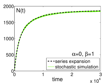
     (a) (b)

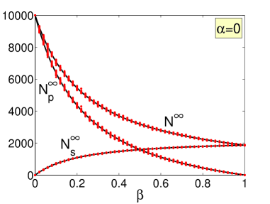
Figure 3: pRSA algorithm for $\alpha=0$. (a) Time evolution of $N(t)$ given by $(\ref{approxNB})$ for $\alpha=0$, $\beta=1$ and $M=100$ (dashed line). Ten realizations of stochastic simulation of pRSA algorithm are plotted as thin solid lines. (b) $N^{\infty}$, $N_{p}^{\infty}$ and $N_{s}^{\infty}$ as obtained by $(\ref{NNsNpinfty})$ (solid lines) for $M=100$. We compare the approximate results with stochastic simulation of pRSA algorithm (20 realizations, each realization plotted as a dot).

We see that approximations (3.13) provide very good results for any $\beta$. We can estimate relative error between approximation $N_{app}^{\infty}$ and exact value $N^{\infty}$ as $(N_{app}^{\infty}-N^{\infty})/N^{\infty}$. Using (3.13), we obtain $N_{app}^{\infty}-N^{\infty}\doteq 2.7$ and $(N_{app}^{\infty}-N^{\infty})/N^{\infty}\doteq 0.15\%$ for $\beta=1$. Here, exact value of $N^{\infty}$ was approximated by averaging over 100,000 realizations of the pRSA algorithm as $N^{\infty}\doteq 1869.8$ for $\beta=1.$

3.2 Special case $\beta=0$

If $\beta=0$, then the pRSA algorithm reduces to the adsorption of point-polymers and cross-polymers. The terms in the sum (2.18) are nonzero only if $\xi(s)=\omega(s)-1$. Hence, (2.18) can be rewritten as

$$\sum_{s\in{\cal Q}_{k}}\alpha^{\omega(s)-1},\qquad\mbox{for}\;k=1,2,3,\dots,$$ (3.14)

where ${\cal Q}_{k}$ is the set of all sequences $s\equiv\{(x_{j},y_{j})\}_{j=1}^{k}$, such that $(x_{1},y_{1})=(1,1)$ and for each $i\in\{2,\dots,k\}$ there exists $j<i$ such that $(x_{i},y_{i})\in{\cal X}_{x_{j},y_{j}}.$ As before, $\omega(s)$ is the number of distinct points in the sequence $s\in{\cal Q}_{k}.$ Using (3.14), we can rewrite (2.17) as

$$N(t)=M^{2}\sum_{k=1}^{\infty}\frac{1}{k!}\left(\frac{t}{M^{2}}\right)^{k}(-1)^{k-1}\sum_{s\in{\cal Q}_{k}}\alpha^{\omega(s)-1}.$$ (3.15)

Comparing formulas (3.3) and (3.15), we find out only two differences: ${\cal P}_{k}$ in (3.3) is replaced by ${\cal Q}_{k}$ in (3.15) and $\beta$ in (3.3) is replaced by $\alpha$ in (3.15). Consequently, taking the Laplace transform of (3.15) and using the same method as in Section 3.1, we find (compare with (3.7))

$$N(t)=\Omega\left(1-\exp\left[-\frac{t}{M^{2}}\right]\right)\quad\mbox{where}\quad\Omega(x)=M^{2}\sum_{k=1}^{\infty}\frac{\left(-\alpha\right)^{k-1}x^{k}}{k!}\Big{|}{\cal H}_{k}\Big{|},$$ (3.16)

where ${\cal H}_{k}$ is the set of all sequences of $k$ distinct points $\{(x_{j},y_{j})\}_{j=1}^{k}$, such that $(x_{1},y_{1})=(1,1)$, and for each $i\in\{2,\dots,k\}$ there exists $j<i$ such that $(x_{i},y_{i})$ is equal to one of the nearest neighbours of $(x_{j},y_{j})$, i.e. $(x_{i},y_{i})\in{\cal X}_{x_{j},y_{j}}$ and $(x_{i},y_{i})\neq(x_{j},y_{j})$. In particular, the final coverage of the lattice can be computed as

$$N^{\infty}\equiv\lim_{t\to\infty}N(t)=\lim_{x\to 1}\Omega(x)$$ (3.17)

and other quantities of interest can be obtained by (2.1), (2.2) and (2.4). Thus, the adsorption algorithm has been transformed to the problem of finding the numbers of sequences in the sets ${\cal H}_{k}$, $k=1,2,\dots.$ Once, we have the numbers $|{\cal H}_{k}|$ we can write $\Omega(x)$ for any $\alpha$ and compute $N(t)$, $N_{p}(t)$, $N_{c}(t)$ and $A(t)$ by (3.16), (2.1) and (2.2), provided that the series in $\Omega(x)$ is convergent. It was pointed out in [6] that the convergence of series (3.16) is slow for $\alpha=1$ and for $x=1$. To overcome this difficulty, we could use Shanks transformation or Padé approximants as in Section 3.1. This approach works in general and we will use it in Section 4 where the general analysis of pRSA algorithm is presented. Here, we present an alternative approach, rewriting series (3.16) in different variables. Several possibilities were shown and motivated in [6]. Here, we write $\Omega(x)$ as

$$\Omega(x(z))=\sum_{k=1}^{\infty}a_{k}z^{k},\qquad\mbox{where}\;\;\;x=\int_{0}^{z}\frac{3}{1+2(1-\xi)^{3}}\mbox{d}\xi.$$ (3.18)

Let us define

$$h_{k}=M^{2}\,\frac{\big{|}{\cal H}_{k}\big{|}}{k!}.$$ (3.19)

To find $h_{k}$, one has to solve a finite combinatorial problem. In this paper, we will make use of the first eight values of $h_{k}$. They can be computed as follow $h_{1}=10000;$ $h_{2}=20000;$ $h_{3}=40000;$ $h_{4}\doteq 73333;$ $h_{5}\doteq 125333;$ $h_{6}\doteq 202222;$ $h_{7}\doteq 311048;$ and $h_{8}\doteq 459452$. To find coefficients $a_{k}$ in (3.18), we substitute $x\equiv x(z)$ in (3.16). We differentiate the resulting series term by term eight times and we evaluate each derivative at $z=0$ to obtain:

$$a_{1} = h_{1}$$

$$a_{2} = h_{1}-\alpha h_{2}$$

$$a_{3} = 2h_{1}/3-2\alpha h_{2}+\alpha^{2}h_{3}$$

$$a_{4} = h_{1}/6-7\alpha h_{2}/3+3\alpha^{2}h_{3}-\alpha^{3}h_{4}$$ (3.20)

$$a_{5} = -4h_{1}/15-5\alpha h_{2}/3+5\alpha^{2}h_{3}-4\alpha^{3}h_{4}+\alpha^{4}h_{5}$$

$$a_{6} = -4h_{1}/9-11\alpha h_{2}/45+11\alpha^{2}h_{3}/2-26\alpha^{3}h_{4}/3+5\alpha^{4}h_{5}-\alpha^{5}h_{6}$$

$$a_{7} = -20h_{1}/63+6\alpha h_{2}/5+53\alpha^{2}h_{3}/15-38\alpha^{3}h_{4}/3+40\alpha^{4}h_{5}/3-6\alpha^{5}h_{6}+\alpha^{6}h_{7}$$

$$a_{8} = 1.852\,\alpha h_{2}-13\alpha^{2}h_{3}/30-63\alpha^{3}h_{4}/5+145\alpha^{4}h_{5}/6-19\alpha^{5}h_{6}+7\alpha^{6}h_{7}-\alpha^{7}h_{8}$$

Let $\overline{z}$ be a solution of equation $1=3\int_{0}^{z}[1+2(1-\xi)^{3}]^{-1}\mbox{d}\xi$ (one can numerically estimate $\overline{z}$ as 0.569). Moreover, let us denote

$$\widetilde{\Omega}(z)=\sum_{k=1}^{8}a_{k}z^{k}$$ (3.21)

where $a_{1}$, …, $a_{8}$ are given by (3.20). Then, using (3.18) and (3.16), we can approximate number of attached polymers as

$$N(t)\approx\widetilde{\Omega}\Big{(}z(t)\Big{)},\;\;\mbox{where $z(t)$ is given by}\;\;1-\exp\left[-\frac{t}{M^{2}}\right]=\int_{0}^{z(t)}\!\!\frac{3}{1+2(1-\xi)^{3}}\mbox{d}\xi.$$ (3.22)

The results obtained by (3.22) for $\alpha=1$ and $M=100$ are given in Figure 4(a). To compute time evolution of $N(t)$, we chose an equidistant mesh in $z$-variable in interval $[0,\overline{z}]$ and evaluated $\widetilde{\Omega}$ by (3.21) at each $z$. The corresponding time $t$ was computed by (3.22), namely using the formula

$$t=-M^{2}\ln\left[1-\int_{0}^{z(t)}\!\!\frac{3}{1+2(1-\xi)^{3}}\mbox{d}\xi\right].$$

In Figure 4(a), we compare results obtained by approximation (3.22) and by stochastic simulation of pRSA algorithm. We get a very good agreement between the theoretically derived formula and simulation. The asymptotic coverage can be approximated as

$$N^{\infty}\equiv\lim_{t\to\infty}N(t)\approx\widetilde{\Omega}(\overline{z}),\quad N^{\infty}_{c}\approx\alpha\,\widetilde{\Omega}(\overline{z}),\quad\mbox{and}\quad N^{\infty}_{p}\approx(1-\alpha)\,\widetilde{\Omega}(\overline{z}).$$ (3.23)

In Figure 4(b), we compare approximations of $N^{\infty}$, $N_{p}^{\infty}$ and $N_{c}^{\infty}$ computed by (3.23) with the results of stochastic simulations.

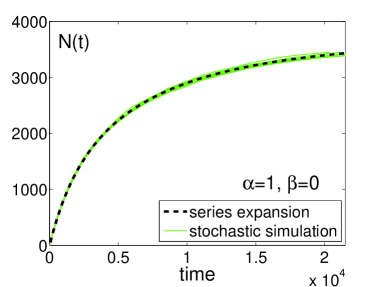
     (a) (b)

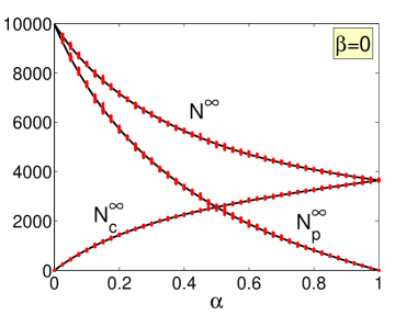
Figure 4: pRSA algorithm for $\beta=0$. (a) Time evolution of $N(t)$ given by $(\ref{approxN})$ for $\alpha=1$, $\beta=0$ and $M=100$ (dashed line). Ten realizations of stochastic simulation of pRSA algorithm are plotted as thin solid lines. (b) $N^{\infty}$, $N_{p}^{\infty}$ and $N_{c}^{\infty}$ as obtained by $(\ref{NNcNpinfty})$ (solid lines) for $M=100$. We compare the approximate results with stochastic simulation of pRSA algorithm (20 realizations, each realization plotted as a dot).

We see that approximations (3.23) provide good results for any $\alpha$. We can estimate relative error between approximation $N_{app}^{\infty}$ and exact value $N^{\infty}$ as $(N_{app}^{\infty}-N^{\infty})/N^{\infty}$. Using (3.23), we obtain $N_{app}^{\infty}-N^{\infty}\doteq 5$ and $(N_{app}^{\infty}-N^{\infty})/N^{\infty}\doteq 0.14\%$ for $\alpha=1$. Here, $N^{\infty}$ can be computed by averaging over many realizations of the pRSA algorithm as $N^{\infty}\doteq 3641$ for $\alpha=1.$

In this section, we used transformation of variables (3.18) to accelerate the convergence of series (3.16). This transformation was suggested in [6] for pRSA algorithm with $[\alpha,\beta]=[1,0]$, but our analysis shows that it can give good results for any $\alpha$. The problem with this approach in general is determining an appropriate change of variables. An easier, and more systematic, approach is to use a Shanks transformation or Padé approximants [15, 20, 19] as we did in Section 3.1, and as we will do for the general analysis of the pRSA algorithm in Section 4.

4 General analysis of pRSA algorithm

To evaluate (2.17) for general $\alpha$ and $\beta$, we have to compute the quantities (2.18) for $k=1,2,3,\dots$. Direct evaluation of (2.18) would require solving different combinatorial problems (weighted sums over all sequences in the set ${\cal P}_{k}$) for different values of $\alpha$ and $\beta$. As in Section 3, we show that a suitable reordering of terms can transform the set of combinatorial problems to only one combinatorial problem which can be solved independently of the values of $\alpha$ and $\beta$. Then the dependence of the number of attached polymers and number of covered binding sites can be easily studied. To do that, we first use the Laplace transform to rewrite (2.17) in terms of ${\cal G}_{k}$. Here, as before ${\cal G}_{k}$ is the set of all sequences of $k$ distinct points $\{(x_{j},y_{j})\}_{j=1}^{k}$, such that $(x_{1},y_{1})=(1,1)$, and for each $i\in\{2,\dots,k\}$ there exists $j<i$ such that $(x_{i},y_{i})\in{\cal S}_{x_{j},y_{j}}$ and $(x_{i},y_{i})\neq(x_{j},y_{j})$. Following a similar analysis to that in Section 3.1, we derive (compare with (3.7))

$$N(t)=\Phi\left(1-\exp\left[-\frac{t}{M^{2}}\right]\right)$$ (4.1)

where

$$\Phi(x)=M^{2}\sum_{k=1}^{\infty}\frac{\left(-1\right)^{k-1}x^{k}}{k!}\sum_{s\in{\cal G}_{k}}[\alpha+\beta]^{\xi(s)}\beta^{k-\xi(s)-1},$$ (4.2)

where, as before, $\xi(s)$ is the number of distinct points $(x_{i},y_{i})\in s,$ $(x_{i},y_{i})\neq(1,1)$, satisfying that there exists $j<i$ such that $(x_{i},y_{i})\in{\cal X}_{x_{j},y_{j}}$. Let $\phi_{j}^{k}$, $j=1,\dots,k$, denote the number of sequences $s\in{\cal G}_{k}$, $k=1,2,\dots,$ satisfying $\xi(s)=k-j.$ The numbers $\phi_{j}^{k}$ for $k=1,2,\dots,8,$ can be directly computed and they are given in Table 1.

$\phi_{j}^{k}$ $j=1$ $j=2$ $j=3$ $j=4$ $j=5$ $j=6$ $j=7$ $j=8$ $k=1$ 1 – – – – – – – $k=2$ 4 4 – – – – – – $k=3$ 24 40 24 – – – – – $k=4$ 176 424 424 176 – – – – $k=5$ 1504 4800 6696 4776 1504 – – – $k=6$ 14560 58368 104752 104280 57640 14560 – – $k=7$ 156768 761024 1677680 2135920 1655336 745064 156768 – $k=8$ ​1852512​ ​​10603744​​ ​​27833952​​ ​​43206736​​ ​​42818768​​ ​​27137992​​ ​​10289192​​ ​1852512​

Table 1: Table of values of $\phi_{j}^{k}$ for $k=1,2,\dots,8$, $j=1,\dots,k$.

Using the definition of $\phi_{j}^{k}$, formula (4.2) can be rewritten to

$$\Phi(x)=M^{2}\sum_{k=1}^{\infty}\frac{\left(-1\right)^{k-1}x^{k}}{k!}\sum_{j=1}^{k}\phi_{j}^{k}[\alpha+\beta]^{k-j}\beta^{j-1}.$$ (4.3)

Our task is to compute the sum of series (4.3) with reasonable precision, using only the first eight partial sums

$$s_{n}(x)=M^{2}\sum_{k=1}^{n}\frac{\left(-1\right)^{k-1}x^{k}}{k!}\sum_{j=1}^{k}\phi_{j}^{k}[\alpha+\beta]^{k-j}\beta^{j-1},\qquad n=1,2,\dots,8.$$

To do that, we use Shanks transformation computed by Wynn’s algorithm (3.1) and we approximate sum $\Phi(x)$ by term $\varepsilon_{7}^{2}(x)$, as in Section 3.1. Thus we aproximate number of attached polymers as

$$N(t)\approx\varepsilon_{7}^{2}\Big{(}x(t)\Big{)},\;\;\mbox{where $x(t)$ is given by}\;\;x(t)=1-\exp\left[-\frac{t}{M^{2}}\right].$$ (4.4)

The asymptotic coverage can be approximated as

$$N^{\infty}\approx\varepsilon_{7}^{2}(1),\quad N^{\infty}_{c}\approx\alpha\,\varepsilon_{7}^{2}(1),\quad N^{\infty}_{s}\approx\beta\,\varepsilon_{7}^{2}(1)\quad\mbox{and}\quad N^{\infty}_{p}\approx(1-\alpha-\beta)\,\varepsilon_{7}^{2}(1).$$ (4.5)

In Figure 5(a), we compare approximations of $N^{\infty}$, $N_{p}^{\infty}$, $N_{c}^{\infty}$ and $N_{s}^{\infty}$ computed by (4.5) with the results of stochastic simulations for $\alpha=0.5$. The same plots for $\beta=0.5$ are given in Figure 5(b). We see that approximations (4.5) provide excellent results.

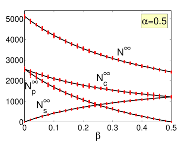
     (a) (b)

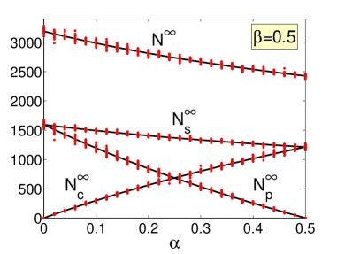
Figure 5: (a) pRSA algorithm for $M=100$ and $\alpha=0.5$; (b) pRSA algorithm for $M=100$ and $\beta=0.5$. In both cases, we present $N^{\infty}$, $N_{p}^{\infty}$, $N_{c}^{\infty}$ and $N_{s}^{\infty}$ as obtained by $(\ref{NNcNsNpinfty})$ (solid lines). We compare the approximate series expansion results with stochastic simulation of pRSA algorithm (20 realizations, each realization plotted as a dot).

The results obtained by (4.4) for $\alpha=0.5$, $\beta=0.5$ and $M=100$ are given in Figure 6. To compute time evolution of $N(t)$, we chose an equidistant mesh in $x$-variable in interval $(0,1)$ and evaluated $\varepsilon_{7}^{2}$ by (3.1) at each $x$. Then the corresponding time $t$ was computed by (4.4). To compute $A(t)$ we used formula (2.2) where the time derivative of $N(t)$ was approximate by the backward-in-time finite difference of $N(t)$. In Figure 6, we compare results obtained by approximation (4.4) and by stochastic simulation of pRSA algorithm. We see that we get a very good agreement between the theoretically derived formula and simulation.

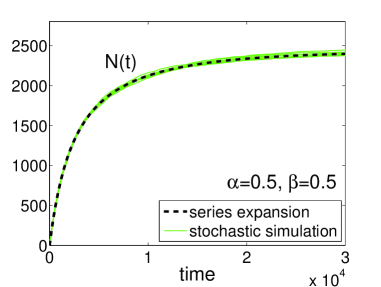
     (a) (b)

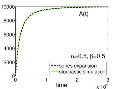
Figure 6: pRSA algorithm for $\alpha=0.5$, $\beta=0.5$ and $M=100$. (a) Time evolution of $N(t)$ given by $(\ref{approxNgen})$ (dashed line). Ten realizations of stochastic simulation of pRSA algorithm are plotted as thin solid lines. (b) Time evolution of $A(t)$ given by $(\ref{approxNgen})$ and $(\ref{obvrelations2})$ (dashed line). Ten realizations of stochastic simulation of pRSA algorithm are plotted as thin solid lines.

Finally, we present the time evolution of $N(t)$ and $A(t)$ for $\alpha=0.8$ and $\beta=0.1$ which is the situation shown in the illustrative computation in Figure 2. In Figure 7, we compare results obtained by (4.4) with results obtained by stochastic simulation of pRSA algorithm. Again, we obtained an excellent agreement between the series expansion results and the stochastic simulation of the pRSA algorithm.

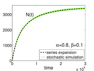
     (a) (b)

Figure 7: pRSA algorithm for $\alpha=0.8$, $\beta=0.1$ and $M=100$. (a) Time evolution of $N(t)$ given by $(\ref{approxNgen})$ (dashed line). Ten realizations of stochastic simulation of pRSA algorithm are plotted as thin solid lines. (b) Time evolution of $A(t)$ given by $(\ref{approxNgen})$ and $(\ref{obvrelations2})$ (dashed line). Ten realizations of stochastic simulation of pRSA algorithm are plotted as thin solid lines.

5 Discussion

In this paper we studied random sequential adsorption to the two-dimensional lattice. Our motivation was chemisorption from polydisperse solution of polymers. We generalized the operator formalism of [1, 5], derived series expansion results and presented efficient methods to accelerate their convergence. In Section 3.1, we used classical methods for accelerating convergence of slowly converging series. In Section 3.2, we also presented results obtained by a more specialized transformation of variables [6]. In both cases, the theoretical results compare well with the results of stochastic simulation of the pRSA algorithm.

We assumed that the attached polymer can effectively shield a circle on the surface with radius $r<2h$ where $h$ is the average distance between neighbouring binding sites. We worked with the rectangular mesh of binding sites to enable the reformulation of the problem in terms of the RSA on the rectangular lattice. One should view this simplification as a reasonable approximation of the problem where binding sites are more or less uniformly distributed on the surface. The restriction $r<2h$ can be also relaxed and the operator formalism could be generalized to the case of a mixture of longer polymers too. However, one should have in mind that for larger $r$, the assumption that the “wiggling tails” of polymers can overlap has to be modified to take into account the higher probability to find the polymer chain close to the binding site; see [2] for the general discussion of the polymer dynamics.

Two-dimensional adsortption is more complicated to study because there is no simple analogy of the exact approach which is available in one-dimension (see e.g. [4] or the integro-differential evolution equation framework which was used in [3]). More precisely, one can formally write an evolution equation for the process (e.g. the master equation denoted (2.9) in this paper) but it can be solved only by various approximation techniques [4]. For example, Nord et al [12] study adsorption of dimers or larger connected sites of objects to two-dimensional lattice. They write a master equation in hierarchic form for conditional probabilities that a conditioned configuration of mesh points is empty given that some neighbouring conditioning sites are empty. Using a series of hierarchic truncation schemes [17], they were able to estimate dynamics and saturating coverage of the adsorption process. The operator formalism presented is a useful alternative to methods based on approximate evolution equations.

The theoretical treatment of irreversible polymer adsorption is given in [13]. They give a more detailed picture than is studied in this paper, by studying the structure of the resulting nonequilibrium layer in terms of the density profiles, and loop and contact fraction distributions. Adsorption of whole polymers to the surface, modelled as a self-avoiding random walk, was done in [18] where the results of Monte Carlo simulations are presented. It has been found that the coverage to its jamming limit is described by a power law $t^{-\gamma}$ where an exponent $\gamma$ depends on the chain length. In our case, we modelled the adsorption of polymers as adsorption of disks to the surface where the binding sites were arranged into the rectangular lattice. In particular, the presented algorithm can be viewed as a generalization of the classical lattice RSA models. Random sequential adsorption has been subject of the intensive research for the last sixty years. The reader can find more details about the RSA in review articles [4] and [16].

References

- [1] R. Dickman, J. Wang, and I. Jensen, Random sequential adsorption: series and virial expansions, Journal of Chemical Physics 94 (1991), no. 12, 8252–8257.
- [2] M. Doi and S. Edwards, The Theory of Polymer Dynamics, Oxford University Press, 1986.
- [3] R. Erban, J. Chapman, K. Fisher, I. Kevrekidis, and L. Seymour, Dynamics of polydisperse irreversible adsorption: a pharmacological example, 22 pages, to appear in Mathematical Models and Methods in Applied Sciences (M3AS), available as arXiv.org/physics/0602001, 2006.
- [4] J. Evans, Random and cooperative sequential adsorption, Reviews of Modern Physics 65 (1993), no. 4, 1281–1329.
- [5] Y. Fan and J. Percus, Asymptotic coverage in random sequential adsorption on a lattice, Physical Review A 44 (1991), no. 8, 5099–5103.
- [6] , Use of model solutions in random sequential adsorption on a lattice, Physical Review Letters 67 (1991), no. 13, 1677–1680.
- [7] K. Fisher, Personal communication, 2005.
- [8] K. Fisher, Y. Stallwood, N. Green, K. Ulbrich, V. Mautner, and Seymour L., Polymer-coated adenovirus permits efficient retargeting and evades neutralising antibodies, Gene therapy 8 (2001), no. 5, 341–348.
- [9] M. Himmelhaus, T. Bastuck, S. Tokumitsu, M Grunze, L. Livadaru, and H.J. Kreuzer, Growth of a dense polymer brush layer from solution, Europhysics letters 64 (2003), no. 3, 378–384.
- [10] I. Kevrekidis, C. Gear, J. Hyman, P. Kevrekidis, O. Runborg, and K. Theodoropoulos, Equation-free, coarse-grained multiscale computation: enabling microscopic simulators to perform system-level analysis, Communications in Mathematical Sciences 1 (2003), no. 4, 715–762.
- [11] S. Milner, T. Witten, and M. Cates, Theory of the grafted polymer brush, Macromolecules 21 (1988), 2610–2619.
- [12] R. Nord and J. Evans, Irreversible immobile random adsorption of dimers, trimers, … on 2D lattices, Journal of Chemical Physics 82 (1985), no. 6, 2795–2810.
- [13] B. O’Shaughnessy and D. Vavylonis, Irreversibility and polymer adsorption, Physical Review Letters 90 (2003), no. 5, 056103.
- [14] , Non-equilibrium in adsorbed polymer layers, Journal of Physics: Condensed Matter 17 (2005), R63–R99.
- [15] D. Shanks, Non-linear transformations of divergent and slowly convergent sequences, J. Math. and Phys. 34 (1955), 1–42.
- [16] J. Talbot, G. Tarjus, P. Van Tassel, and P. Viot, From car parking to protein adsorption: An overview of sequential adsorption processes, Colloids and Surfaces A: Physicochemical and Engineering Aspects 165 (2000), 287–324.
- [17] K. Vette, T. Orent, D. Hoffman, and R. Hansen, Kinetic model for dissociative adsorption of a diatomic gas, Journal of Chemical Physics 60 (1974), no. 12, 4854–4861.
- [18] J. Wang and R. Pandey, Kinetics and jamming coverage in a random sequential adsorption of polymer chains, Physical Review Letters 77 (1996), no. 9, 1773–1776.
- [19] E. Weniger, Nonlinear sequence transformations for the acceleration of convergence and the summation of divergent series, Comput. Phys. Rep. 10 (1989), 189–371.
- [20] P. Wynn, On a device for computing the transformation, Math. Tables Aids Comput. 10 (1956), 91–96.
- [21] R. Zajac and A. Chakrabarti, Kinetics and thermodynamics of end-functionalized polymer adsorption and desorption processes, Physical Review E 49 (1994), no. 4, 3069–3078.