A Generalized Preferential Attachment Model for Business Firms Growth Rates: II. Mathematical Treatment

Abstract

We present a preferential attachment growth model to obtain the distribution $P(K)$ of number of units $K$ in the classes which may represent business firms or other socio-economic entities. We found that $P(K)$ is described in its central part by a power law with an exponent $\varphi=2+b/(1-b)$ which depends on the probability of entry of new classes, $b$. In a particular problem of city population this distribution is equivalent to the well known Zipf law. In the absence of the new classes entry, the distribution $P(K)$ is exponential. Using analytical form of $P(K)$ and assuming proportional growth for units, we derive $P(g)$, the distribution of business firm growth rates. The model predicts that $P(g)$ has a Laplacian cusp in the central part and asymptotic power-law tails with an exponent $\zeta=3$. We test the analytical expressions derived using heuristic arguments by simulations. The model might also explain the size-variance relationship of the firm growth rates.

I Introduction

Gibrat Gibrat30 ; Gibrat31 , building upon the work of the astronomer Kapteyn Kapteyn16 , assumed the expected value of the growth rate of a business firm’s size to be proportional to the current size of the firm, which is called “Law of Proportionate Effect” Zipf49 ; Gabaix99 . Several models of proportional growth have been subsequently introduced in economics in order to explain the growth of business firms Steindl65 ; Sutton97 ; Kalecki45 . Simon and co-authors Simon55 ; Simon58 ; Simon75 ; Simon77 extended Gibrat’s model by introducing an entry process according to which the number of firms rise over time. In Simon’s framework, the market consists of a sequence of many independent “opportunities” which arise over time, each of size unity. Models in this tradition have been challenged by many researchers Stanley96 ; Lee98 ; Stanley99 ; Bottazzi01 ; Matia04 who found that the firm growth distribution is not Gaussian but displays a tent shape.

Here we introduce a mathematical framework that provides an unifying explanation for the growth of business firms based on the number and size distribution of their elementary constituent components Amaral97 ; Sergey_II ; Sutton02 ; DeFabritiis03 ; Amaral98 ; Takayasu98 ; Canning98 ; Buldyrev03 . Specifically we present a model of proportional growth in both the number of units and their size and we draw some general implications on the mechanisms which sustain business firm growth Simon75 ; Sutton97 ; Kalecki ; Mansfield ; Hall ; DeFabritiis03 . According to the model, the probability density function (PDF) of growth rates, $P(g)$ is Laplace Kotz01 in the center Stanley96 with power law tails Reed01 ; Reed02 decaying as $g^{-\zeta}$ where $\zeta=3$.

Two key sets of assumptions in the model are described in subsections A (the number of units $K$ in a class grows in proportion to the existing number of units) and B (the size of each unit fluctuates in proportion to its size). Our goal is to first find $P(K)$, the probability distribution of the number of units in the classes at large $t$, and then find $P(g)usingtheconvolutionof$P(K) and the conditional distribution of the class growth rates $P(g|K)$, which for large $K$ converges to a Gaussian..

II Analytical Results

II.1 The Proportional Growth of Number of Units

The first set of assumptions Kazuko is:

• Each class $\alpha$ consists of $K_{\alpha}(t)$ number of units. At time $t=0$, there are $N(0)$ classes consisting of $n(0)$ total number of units. The initial average number of units in a class is thus $n(0)/N(0)$.

• At each time step a new unit is created. Thus the number of units at time $t$ is $n(t)=n(0)+t$.

• With birth probability $b$, this new unit is assigned to a new class, so that the average number of classes at time $t$ is $N(t)=N(0)+bt$.

• With probability $1-b$, a new unit is assigned to an existing class $\alpha$ with probability $P_{\alpha}=(1-b)K_{\alpha}(t)/n(t)$, so $K_{\alpha}(t+1)=K_{\alpha}(t)+1$.

This model can be generalized to the case when the units are born at any unit of time $t^{\prime}$ with probability $\mu$, die with probability $\lambda$, and in addition a new class consisting of one unit can be created with probability $b^{\prime}$ Kazuko . This model can be reduced to the present model if one introduce time $t=t^{\prime}(\mu-\lambda+b^{\prime})$ and probability $b=b^{\prime}/(\mu-\lambda+b^{\prime})$.

Our goal is to find $P(K)$, the probability distribution of the number of units in the classes at large $t$. This model in two limiting cases (i) $b=0$, $K_{\alpha}=1$ $(\alpha=1,2\ldots N(0))$ and (ii) $b\neq 0$, $N(0)=1$, $n(0)=1$ has exact analytical solutions $P(K)=N(0)/t(t/(t+N(0)))^{K}(1+O(1/t))$ Johnson ; Kotz2000 and $\lim\limits_{t\to\infty}P(K)=(1+b)\Gamma(K)\Gamma(2+b)/\Gamma(K+2+b)$ Reed04 respectively, In general, an exact analytical solution of this problem cannot be presented in a simple close form. Accordingly, we seek for an approximate mean-field type book solution which can be expressed in simple integrals and even in elementary functions in some limiting cases. First we will present a known solution of the preferential attachment model in the absence of the influx of new classes Cox :

$$P_{\rm old}(K)=\lambda^{K}\frac{1}{K(t)-1}\approx\frac{1}{K(t)}\exp(-K/K(t))[1+O(t^{-1})],$$ (1)

where $\lambda=1-1/K(t)$ and $K(t)=[n(0)+t]/N(0)$ is the average number of units in the old classes at time $t$. Note that the form of the distribution of units in the old classes remains unchanged even in the presence of the new classes, whose creation does not change the preferential attachment mechanism of the old classes and affects only the functional form of $K(t)$.

Now we will treat the problem in the presence of the influx of the new classes. Assume that at the beginning there are $N(0)$ classes with $n(0)$ units. Because at every time step, one unit is added to the system and a new class is added with probability $b$, at moment $t$ there are

$$n(t)=n(0)+t$$ (2)

units and approximately

$$N(t)=N(0)+bt$$ (3)

classes, among which there are approximately $bt$ new classes with $n_{new}$ units and $N(0)$ old classes with $n_{old}$ units, such that

$$n_{old}+n_{new}=n(0)+t.$$ (4)

Because of the preferential attachment assumption (A4), we can write, neglecting fluctuations book and assuming that $t$, $n_{old}$, and $n_{new}$ are continuous variables:

$$\frac{dn_{new}}{dt} = b+(1-b)\frac{n_{new}}{n(0)+t},$$ (5)

$$\frac{dn_{old}}{dt} = (1-b)\frac{n_{old}}{n(0)+t}.$$ (6)

Solving the second differential equation and taking into account initial condition $n_{old}(0)=n(0)$, we obtain $n_{old}(t)=(n(0)+t)^{1-b}\,\,n(0)^{b}$. Analogously, the number of units at time $t$ in the classes existing at time $t_{0}$ is

$$n_{e}(t_{0},t)=(n(0)+t)^{1-b}(n(0)+t_{0})^{b}$$ (7)

where the subscript ‘e’ means “existing”. Accordingly, the average number of units in old classes is

$$K(t)=\frac{n_{old}(t)}{N(0)}=\frac{(n(0)+t)^{1-b}}{N(0)}\,\,n(0)^{b}.$$ (8)

Thus according to Eq. (1), the distribution of units in the old classes is

$$P_{old}(K)\approx\frac{N(0)}{(n(0)+t)^{1-b}n(0)^{b}}\,\,\,\exp\left(-\frac{K\,N(0)}{(n(0)+t)^{1-b}n(0)^{b}}\right).$$ (9)

and the contribution of the old classes to the distribution of all classes is

$$\tilde{P}_{old}(K)=P_{old}(K)N(0)/(N(0)+bt).$$ (10)

The number of units in the classes that appear at $t_{0}$ is $b\,dt$ and the number of these classes is $b\,dt$. Because the probability that a class captures a new unit is proportional to the number of units it has already gotten at time $t$, the number of units in the classes that appear at time $t_{0}$ is

$$n_{new}(t_{0},t)=n_{e}(t_{0},t)bdt/[n(0)+t_{0}].$$ (11)

The average number of units in these classes is

$$K(t_{0},t)=n_{new}(t_{0},t)/b\,dt=(n(0)+t)^{1-b}/(n(0)+t_{0})^{1-b}.$$ (12)

Assuming that the distribution of units in these classes is given by a continuous approximation (1) we have

$$P_{new}(K,t_{0})\approx\frac{1}{K(t_{0},t)}\,\exp\left(-K/K(t_{0},t)\right).$$ (13)

Thus, their contribution to the total distribution is

$$\frac{b\,dt_{0}}{N(0)+b\,t}\,\frac{1}{K(t_{0},t)}\,\exp\left(-K/K(t_{0},t)\right)$$

The contribution of all new classes to the distribution $P(K)$ is

$$\tilde{P}_{new}(K)\approx\frac{b}{N(0)+b\,t}\int_{0}^{t}\frac{1}{K(t_{0},t)}\,\exp\left(-K/K(t_{0},t)\right)\,dt_{0}.$$ (14)

If we let $y=K/K(t_{0},t)$ then $\tilde{P}_{new}(K)=P_{new}(K)bt/(N(0)+bt)$ where

$$P_{new}(K) \approx \frac{n(0)/t+1}{1-b}\,\,K^{\left(-\frac{1}{1-b}-1\right)}\,\,\int^{K}_{K^{\prime}}e^{-y}\,\,y^{\frac{1}{1-b}}\,\,dy.$$ (15)

and the low limit of integration, $K^{\prime}$ is given by

$$K^{\prime}=K\left(\frac{n(0)}{n(0)+t}\right)^{1-b}$$ (16)

Finally the distribution of units in all classes is given by

$$P(K)=\frac{N(0)}{N(0)+bt}\,P_{old}(K)\,+\,\frac{bt}{N(0)+bt}\,P_{new}(K).$$ (17)

Now we investigate the asymptotic behavior of the distribution in Eq. (15) and show that it can be described by the Pareto power law tail with an exponential cut-off.

1. At fixed $K$ when $t\rightarrow\infty$, we have $K^{\prime}\to 0$, thus

$$P_{new}(K) = \frac{1}{1-b}\,\,K^{-\frac{1}{1-b}-1}\int_{0}^{K}e^{-y}\,\,y^{\frac{1}{1-b}}\,\,dy,$$ (18)

$$= \frac{1}{1-b}\,\left[\Gamma\left(1+\frac{1}{1-b}\right)-\int_{K}^{\infty}e^{-y}\,\,y^{\frac{1}{1-b}}\,\,dy\right]\,\,K^{-1-\frac{1}{1-b}}.$$

As $K\rightarrow\infty$, $P_{new}(K)$ converges to a finite value:

$$P_{new}(K) = K^{-1-\frac{1}{b}}\left(\frac{1}{1-b}\right)\,\,\Gamma\left(1+\frac{1}{1-b}\right).$$ (19)

Thus for large $K\gg 1$, but such that $K^{\prime}\ll 1$ or $K\ll(1+t/n(0)^{1-b}$, we have an approximate power-law behavior:

$$P_{new}(K)\sim K^{-\varphi},$$ (20)

where $\varphi=2+b/(1-b)\geq 2$.

As $K\rightarrow 0$,

$$P_{new}(K) = \frac{1}{1-b}\,\,K^{\left(-\frac{1}{1-b}-1\right)}\,\,\frac{K^{\left(1+\frac{1}{1-b}\right)}}{1+\frac{1}{1-b}}=\frac{1}{2-b}.$$ (21)

2. At fixed $t$ when $K\rightarrow\infty$, we use the partial integration to evaluate the incomplete $\Gamma$ function:

$$\,\,\,\,\,\,\int_{x}^{\infty}e^{-y}\,\,y^{\alpha}\,\,dy = -e^{-y}\,\,y^{\alpha}|_{x}^{\infty}+\alpha\int_{x}^{\infty}e^{-y}\,\,y^{\alpha-1}\,\,dy\approx e^{-x}\,\,x^{\alpha}.$$

Therefore, from Eq. (15) we obtain

$$\tilde{P}_{new}(K) \approx \frac{n(0)+t}{N(0)+bt}\,\,\frac{b}{1-b}\,\,K^{-\frac{1}{1-b}-1}\int^{\infty}_{K\left(\frac{n(0)}{n(0)+t}\right)^{1-b}}\,\,e^{-y}\,\,y^{\frac{1}{1-b}}\,\,dy,$$ (22)

$$= \frac{n(0)}{N(0)+bt}\,\,\frac{b}{1-b}\,\,\frac{1}{K}\,\,\exp\left(-K\left(\frac{n(0)}{n(0)+t}\right)^{1-b}\right),$$

which always decays faster than Eq. (9) because $n(0)\geq N(0)$ and there is an additional factor $K^{-1}$ in front of the exponential. Thus the behavior of the distribution of all classes is dominated for large $K$ by the exponential decay of the distribution of units in the old classes.

Note that Eq. (9) and Eq. (15) are not exact solutions but continuous approximations which assume $K$ is a real number. This approximation produces the most serious discrepancy for small $K$. To test this approximation, we perform numerical simulations of the model for $b=0.1$, $N(0)=n(0)=10000$ and $t=400000$. The results are presented in Fig.1. While the agreement is excellent for large $K$, Eq. (15) significantly underestimates the value of $\tilde{P}_{new}(K)$ for $K=1$ and $K=2$. Note that in reality the power-law behavior of $\tilde{P}_{new}(K)$ extends into the region of very small $K$.

II.2 The Proportional Growth of Size of Units

The second set of assumptions of the model is:

• At time $t$, each class $\alpha$ has $K_{\alpha}(t)$ units of size $\xi_{i}(t)$, ${i=1,2,...K_{\alpha}(t)}$ where $K_{\alpha}$ and $\xi_{i}>0$ are independent random variables taken from the distributions $P(K_{\alpha})$ and $P_{\xi}(\xi_{i})$ respectively. $P(K_{\alpha})$ is defined by Eq. (17) and $P_{\xi}(\xi_{i})$ is a given distribution with finite mean and standard deviation and $\ln\xi_{i}$ has finite mean $\mu_{\xi}=\langle\ln\xi_{i}\rangle$ and variance $V_{\xi}=\langle(\ln\xi_{i})^{2}\rangle-\mu_{\xi}^{2}$. The size of a class is defined as $S_{\alpha}(t)\equiv\sum_{i=1}^{K_{\alpha}}\xi_{i}(t)$.

• At time $t+1$, the size of each unit is decreased or increased by a random factor $\eta_{i}(t)>0$ so that

  $$\xi_{i}(t+1)=\xi_{i}(t)\,\eta_{i}(t),$$ (23)

  where $\eta_{i}(t)$, the growth rate of unit $i$, is independent random variable taken from a distribution $P_{\eta}(\eta_{i})$, which has finite mean and standard deviation. We also assume that $\ln\eta_{i}$ has finite mean $\mu_{\eta}\equiv\langle\ln\eta_{i}\rangle$ and variance $V_{\eta}\equiv\langle(\ln\eta_{i})^{2}\rangle-\mu_{\eta}^{2}$.

Let us assume that due to the Gibrat process, both the size and growth of units ($\xi_{i}$ and $\eta_{i}$ respectively) are distributed lognormally

$$p(\xi_{i})={\frac{1}{\sqrt{2\pi V_{\xi}}}}\,\,{\frac{1}{\xi_{i}}}\,\,\exp\left(-(\ln\xi_{i}-m_{\xi})^{2}/2V_{\xi}\right),$$ (24)

$$p(\eta_{i})={\frac{1}{\sqrt{2\pi V_{\eta}}}}\,\,{\frac{1}{\eta_{i}}}\,\,\exp\left(-(\ln\eta_{i}-m_{\eta})^{2}/2V_{\eta}\right).$$ (25)

If units grow according to a multiplicative process, the size of units $\xi_{i}^{\prime}=\xi_{i}\eta_{i}$ is distributed lognormally with $V_{\xi^{\prime}}=V_{\xi}+V_{\eta}$ and $m_{\xi^{\prime}}=m_{\xi}+m_{\eta}$.

The $n^{\mbox{\scriptsize th}}$ moment of the variable $x$ distributed lognormally is given by

$$\mu_{x}(n) = \int_{0}^{\infty}{\frac{1}{\sqrt{2\pi V}}}\,{\frac{x^{n}}{x}}\,dx\,\exp\left(-(\ln x-m)^{2}/2V\right)\,\,=\,\,\exp\left(nm_{x}+n^{2}V_{x}/2\right).$$ (26)

Thus, its mean is $\mu_{x}\equiv\mu_{x}(1)=\exp(m_{x}+V_{x}/2)$ and its variance is $\sigma_{x}^{2}\equiv\mu_{x}(2)-\mu_{x}(1)^{2}=\mu_{x}(1)^{2}\,(\exp(V_{x})-1)$.

Let us now find the distribution of $g$ growth rate of classes. It is defined as

$$g\equiv\ln{\frac{S(t+1)}{S(t)}}=\ln\sum_{i=1}^{K}\xi_{i}^{\prime}-\ln\sum_{i=1}^{K}\xi_{i}.$$ (27)

Here we neglect the influx of new units, so $K_{\alpha}=K_{\alpha}(t+1)=K_{\alpha}(t)$.

The resulting distribution of thegrowth rates of all classes is determined by

$$P(g)\equiv\sum_{K=1}^{\infty}P(K)P(g|K),$$ (28)

where $P(K)$ is the distribution of the number of units in the classes, computed in the previous stage of the model and $P(g|K)$ is the conditional distribution of growth rates of classes with given number of units determined by the distribution $P_{\xi}(\xi)$ and $P_{\eta}(\eta)$.

Now our goal is to find an analytical approximation for $P(g|K)$. According to the central limit theorem, the sum of $K$ independent random variables with mean $\mu_{\xi}\equiv\mu_{\xi}(1)$ and finite variance $\sigma_{\xi}^{2}$ is

$$\sum_{i=1}^{K}\xi_{i}=K\mu_{\xi}+\sqrt{K}\nu_{K},$$ (29)

where $\nu_{K}$ is the random variable with the distribution converging to Gaussian

$$\lim_{K\to\infty}P(\nu_{K})\to{\frac{1}{\sqrt{2\pi\sigma_{\xi}^{2}}}}\,\,\exp\left(-\nu_{K}^{2}/2\sigma_{\xi}^{2}\right).$$ (30)

Accordingly, we can replace $\ln(\sum_{i=1}^{K}\xi_{i})$ by its Tailor’s expansion $\ln K+\ln\mu_{\xi}+\nu_{K}/(\mu_{\xi}\sqrt{K})$, neglecting the terms of order $K^{-1}$. Because $\ln\mu_{\eta}=m_{\eta}+V_{\eta}/2$ and $\ln\mu_{\xi^{\prime}}=\ln\mu_{\xi}+\ln\mu_{\eta}$ we have

$$g\equiv\ln S(t+1)-\ln S(t) = \ln(K\mu_{\xi^{\prime}})+{\frac{\nu_{K}^{\prime}}{\sqrt{K}\mu_{\xi^{\prime}}}}-\ln(K\mu_{\xi})-{\frac{\nu_{K}}{\sqrt{K}\mu_{\xi}}},$$ (31)

$$= m_{\eta}+{\frac{V_{\eta}}{2}}+{\frac{\nu_{K}^{\prime}\mu_{\xi}-\nu_{K}\mu_{\xi^{\prime}}}{\sqrt{K}\mu_{\xi}\mu_{\xi^{\prime}}}}.$$

For large $K$ the last term in Eq. (31) is the difference of two Gaussian variables and that is a Gaussian variable itself. Thus for large $K$, $g$ converges to a Gaussian with mean, $m=m_{\eta}+V_{\eta}/2$, and certain standard deviation which we must find.

In order to do this, we rewrite

$$\frac{\nu_{K}^{\prime}}{\sqrt{K}\,\mu_{\xi^{\prime}}}=\frac{\sum_{i=1}^{K}(\xi_{i}^{\prime}-\mu_{\xi^{\prime}})}{K\,\mu_{\xi^{\prime}}},$$

and

$$\frac{\nu_{K}}{\sqrt{K}\,\mu_{\xi}}=\frac{\sum_{i=1}^{K}(\xi_{i}-\mu_{\xi})}{K\,\mu_{\xi}}.$$

Thus

$$g = m_{\eta}+{\frac{V_{\eta}}{2}}\,+\,{\frac{\sum_{i=1}^{K}\xi_{i}(\eta_{i}\mu_{\xi}-\mu_{\xi^{\prime}})}{K\mu_{\xi}\mu_{\xi^{\prime}}}},$$ (32)

$$= m_{\eta}+{\frac{V_{\eta}}{2}}+{\frac{\sum_{i=1}^{K}\xi_{i}(\eta_{i}-\mu_{\eta})}{K\mu_{\xi^{\prime}}}}.$$

Since $\mu_{\xi^{\prime}}=\mu_{\xi}\mu_{\eta}$, the average of each term in the sum is $\mu_{\xi^{\prime}}-\mu_{\xi}\,\mu_{\eta}=0$. The variance of each term in the sum is $\langle(\xi_{i}\,\eta_{i})^{2}\rangle-\langle 2\xi_{i}^{2}\,\eta_{i}\,\mu_{\eta}\rangle+\langle\xi_{i}^{2}\,\mu_{\eta}^{2}\rangle$ where $\xi_{i}\eta_{i}$, $\xi_{i}^{2}\eta_{i}$ and $\xi_{i}^{2}$ are all lognormal independent random variables. Particularly, $(\xi_{i}\eta_{i})^{2}$ is lognormal with $V=4V_{\eta}+4V_{\xi}$ and $m=2m_{\eta}+2m_{\xi}$; $\xi_{i}^{2}\eta_{i}$ is lognormal with $V=4V_{\xi}+V_{\eta}$ and $m=2m_{\xi}+m_{\eta}$; $\xi_{i}^{2}$ is lognormal with $V=4V_{\xi}$ and $m=2m_{\xi}$. Using Eq. (26)

$$\langle(\xi_{i}\eta_{i})^{2}\rangle =\exp(2m_{\eta}+2m_{\xi}+2V_{\eta}+2V_{\xi}),$$ (33a)

$$\langle\xi_{i}^{2}\eta_{i}\rangle =\exp(m_{\eta}+2m_{\xi}+2V_{\xi}+V_{\eta}/2),$$ (33b)

$$\langle\xi_{i}^{2}\rangle =\exp(2m_{\xi}+2V_{\xi}).$$ (33c)

Collecting all terms in Eqs. (33a-33c) together and using Eq. (32) we can find the variance of $g$:

$$\sigma^{2} = \frac{K\,\exp(2m_{\xi}+2V_{\xi}+2m_{\eta}+V_{\eta})(\exp(V_{\eta})-1)}{K^{2}\exp(2m_{\xi}+V_{\xi}+2m_{\eta}+V_{\eta})},$$ (34)

$$= \frac{1}{K}\exp(V_{\xi})\,(\exp(V_{\eta})-1).$$

Therefore, for large $K$, $g$ has a Gaussian distribution

$$P(g|K)={\frac{\sqrt{K}}{\sqrt{2\pi V}}}\,\exp\left(-\frac{(g-m)^{2}K}{2V}\right),$$ (35)

where

$$m=m_{\eta}+V_{\eta}/2$$ (36)

and

$$V\equiv K\sigma^{2}=\exp(V_{\xi})(\exp(V_{\eta})-1).$$ (37)

Note, that the convergence of the sum of lognormals to the Gaussian given by Eq. (29) is a very slow process, achieving reasonable accuracy only for $K\gg\mu_{\xi}(2)\sim\exp(2V_{\xi})$. For a pharmaceutical database Fu_PNAS , we have $V_{\xi}=5.13$, $m_{\xi}=3.44$, $V_{\eta}=0.36$, and $m_{\eta}=0.16$. Accordingly, we can expect convergence only when $K\gg 3\cdot 10^{4}$. Figure2 demonstrates the convergence of the normalized variance $K\sigma^{2}(K)$ and mean $m(K)$ of $g$ to the theoretical limits given by Eqs. (36) and (37) respectively: $V=73.24$ and $m=0.196$. In both cases, the discrepancy between the limiting values and the actual values decreases as $1/\sqrt{K}$. Interestingly, Eq. (35) predicts $\sigma(K)\sim K^{-\beta}$, where $\beta=1/2$. This value is much larger than the empirical value $\beta\approx 0.2$ observed for the size-variance relationships of various socio-economic entities Stanley96 ; Amaral97 ; Sergey_II ; Matia05 . However, the slow convergence of $V(K)K$ suggests that for quite a wide range of $K<1000$, $\sigma(K)\sim K^{-0.2}$ and only at $K>10^{4}$ there is a crossover to the theoretical value $\beta=0.5$, (Fig. 3). Finally, the simulated distribution of $P(g|K)$ has tent-shape wings which develop as $K$ increases (Fig. 4). This feature of the model growth rates may explain the abundance of the tent-shaped wings of the growth rates of various systems in nature. The most drastic discrepancy between the Gaussian shape and the simulated distribution $P(g|K)$ can be seen when $K\approx 1000$ and than it starts to decrease slowly, and remains visible even for $K=10^{6}$.

Nevertheless, in order to obtain close form approximations for the growth rate, we will use the Gaussian approximation (35) for $P(g|K)$. The distribution of the growth rate of the old classes can be found by Eq. (28). In order to find a close form approximation, we replace the summation in Eq. (28) by integration and replace the distributions $P(K)$ by Eq. (9) and $P(g|K)$ by the Eq. (35). Assuming $m=0$, we have

$$P_{old}(g) \approx {\frac{1}{\sqrt{2\pi V}}}\int_{0}^{\infty}{\frac{1}{K(t)}}\,\exp(\frac{-K}{K(t)})\exp(-\frac{g^{2}\,K}{2\,V})\sqrt{K}\,\,dK,$$ (38)

$$= \frac{\sqrt{K(t)}}{2\,\sqrt{2\,V}}\,\left(1+\frac{K(t)}{2V}\,g^{2}\right)^{-\frac{3}{2}},$$

where $K(t)$ is the average number of units in the old classes (see Eq. (8)). This distribution decays as $1/g^{3}$ and thus does not have a finite variance. In spite of drastic assumptions that we make, Eq. (38) correctly predicts the shape of the convolution $P_{old}(g)$. Figure 5 shows the comparison of the simulation of the growth rates in the system with the exponential distribution of units $P(K)$ with $K(t)=2^{15}$ and the same empirical parameters of the unit size and growth distributions as before. The parameter of the analytical distribution characterizing its width (variance does not exist), must be taken $V=33$ which is much smaller than the analytical prediction $V=73.23$. This is not surprising, since for $K=2^{15}$ $K\sigma^{2}(K)=50$ (see Fig. 2b). Moreover, since we are dealing with the average $\sigma^{2}(K)K$ for $K<2^{15}$, we can expect $V<50$. Nevertheless the nature of the power-law wings decaying as $1/g^{3}$ is reproduced very well.

For the new classes, when $t\to\infty$ the distribution of number of units is approximated by

$$P_{\mbox{\scriptsize new}}(K)\approx{\frac{1}{1-b}}K^{-1-\frac{1}{1-b}}\,\int_{0}^{K}\,y^{\frac{1}{1-b}}\,e^{-y}\,\,dy.$$ (39)

Again replacing summation in Eq. (28) in the text by integration and $P(g|K)$ by Eq. (35) and after the switching the order of integration we have:

$$P_{new}(g)\approx{\frac{1}{1-b}}\,{\frac{1}{\sqrt{2\pi V}}}\int_{0}^{\infty}\,\exp(-y)\,y^{\frac{1}{1-b}}\,dy\,\int_{y}^{\infty}\,\exp(-g^{2}\,K/2V)\,K^{(-\frac{1}{2}-\frac{1}{1-b})}\,dK.$$ (40)

As $g\to\infty$, we can evaluate the second integral in Eq. (40) by partial integration:

$$P_{new}(g) \approx \frac{1}{1-b}\int_{0}^{\infty}\frac{1}{\sqrt{2\pi V}}\,\,\frac{2V}{g^{2}}\,\,y^{-\frac{1}{1-b}-\frac{1}{2}}\,\,y^{\frac{1}{1-b}}\,\,\exp(-y)\,\,\exp(-y\,g^{2}/2V)\,\,dy,$$ (41)

$$= \frac{1}{1-b}\,\frac{1}{\sqrt{2\pi V}}\,\frac{2V}{g^{2}}\,\,\frac{1}{\sqrt{g^{2}/2V+1}}\,\,\sqrt{\pi}\sim\frac{1}{g^{3}}.$$

We can compute the first derivative of the distribution (40) by differentiating the integrand in the second integral with respect to $g$. The second integral converges as $y\to 0$, and we find the behavior of the derivative for $g\to 0$ by the substitution $x=Kg^{2}/(2V)$. As $g\to 0$, the derivative behaves as $g\,g^{2[-(3/2)+1/(1-b)]}\sim g^{2b/(1-b)}$, which means that the function itself behaves as $C_{2}-C_{1}|g|^{2b/(1-b)+1}$, where $C_{2}$ and $C_{1}$ are positive constants. For small $b$ this behavior is similar to the behavior of a Laplace distribution with variance $V$: $\exp(-\sqrt{2}|g|/\sqrt{V})/\sqrt{2V}=1/\sqrt{2V}-|g|/V$.

When $b\to 0$, Eq. (40) can be expressed in elementary functions:

$$P_{new}(g)|_{b\to 0} \approx \frac{1}{\sqrt{2\pi V}}\,\int_{0}^{\infty}K^{-3/2}\,\exp(-K\,g^{2}/2\,V)\,dK\,\int_{0}^{K}\,\exp(-y)\,y\,\,dy,$$

$$\approx \frac{1}{\sqrt{2\,V}}\,\,\left(-\frac{1}{\sqrt{1+g^{2}/2\,V}}+\frac{2}{|g|/\sqrt{2\,V}+\sqrt{g^{2}/2\,V+1}}\right).$$

Simplifying we find the main result:

$$P_{\mbox{\scriptsize new}}(g)|_{b\to 0}\approx\frac{2V}{\sqrt{g^{2}+2V}\,(|g|+\sqrt{g^{2}+2V})^{2}}.$$ (42)

which behaves for $g\to 0$ as $1/\sqrt{2V}-|g|/V$ and for $g\to\infty$ as $V/(2g^{3})$. Thus the distribution is well approximated by a Laplace distribution in the body with power-law tails. Because of the discrete nature of the distribution of the number of units, when $g\gg\sqrt{2V}$ the behavior for $g\to\infty$ is dominated by $\exp(-g^{2}/2V)$.

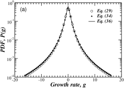
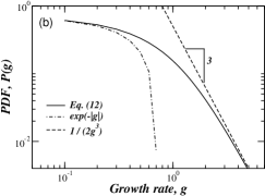
Figure 6: (a) Comparison of three different approximations for the growth rate PDF, $P(g)$, given by Eq. (38), mean field approximation Eq. (40) for $b=0.1$ and Eq. (42). Each $P(g)$ shows similar tent shape behavior in the central part. We see there is little difference between the three cases, $b=0$ (no entry), $b=0.1$ (with entry) and the mean field approximation. This means that entry of new classes ($b>0$) does not perceptibly change the shape of $P(g)$. Note that we use $K(t)/V_{g}=2.16$ for Eq. (38) and $V_{g}=1$ for Eq. (42). (b) The crossover of $P(g)$ given by Eq. (42) between the Laplace distribution in the center and power law in the tails. For small $g$, $P(g)$ follows a Laplace distribution $P(g)\sim\exp(-|g|)$, and for large $g$, $P(g)$ asymptotically follows an inverse cubic power law $P(g)\sim g^{-3}$.

In Fig. 6a we compare the distributions given by Eq. (38), the mean field approximation Eq. (40) for $b=0.1$ and Eq. (42) for $b\to 0$. We find that all three distributions have very similar tent shape behavior in the central part. In Fig. 6b we also compare the distribution Eq. (42) with its asymptotic behaviors for $g\to 0$ (Laplace cusp) and $g\to\infty$ (power law), and find the crossover region between these two regimes.

III Conclusions

The analytical solution of this model can be obtained only for certain limiting cases but a numerical solution can be easily computed for any set of assumptions. We investigate the model numerically and analytically (see and find:

• In the presence of the influx of new classes ($b>0$), the distribution of units converges for $t\to\infty$ to a power law $P(K)\sim K^{-\varphi}$, $\varphi=2+b/(1-b)\geq 2$. Note that this behavior of the power-law probability density function leads to the power law rank-order distribution where rank of a class $R$ is related to the number of its units $K$ as

  $$R=N(t)\int_{K}^{\infty}P(K)dk\sim K^{-\varphi+1}.$$ (43)

  Thus $K\sim R^{-\zeta}$, where $\zeta=1/(\varphi-1)=1-b\leq 1$, which leads in the limit $b\to 0$ to the celebrated Zipf’s lawZipf49 for cities populations, $K\sim 1/R$. Note that this equation can be derived for our model using elementary considerations. Indeed, due to proportional growth the rank of a class, $R$, is proportional to the time of its creation $t_{0}$. The number of units $n(t_{0})$ existing at time $t_{0}$ is also proportional to $t_{0}$ and thus also proportional to $R$. According to the proportional growth, the ratio of the number of units in this class to the number of units in the classes existed at time $t_{0}$ is constant: $K(t_{0},t)/n_{e}(t_{0},t)=1/n(t_{0})$. If we assume that the amount of units in the classes, created after $t_{0}$ can be neglected since the influx of new classes $b$ is small, we can approximate $n_{e}(t_{0},t)\approx n(t)\sim t$. Thus for large $t$, $n_{e}(t_{0},t)$ is independent of $t_{0}$ and hence $K(t_{0},t)\sim 1/R$. If we do not neglect the influx of new classes, Eq. (7) gives $n_{e}(t_{0},t)\sim t_{0}^{b}$, hence $K(t_{0},t)\sim 1/R^{1-b}$.

• The conditional distribution of the logarithmic growth rates $P(g|K)$ for the classes consisting of a fixed number $K$ of units converges to a Gaussian distribution (35) for $K\to\infty$. Thus the width of this distribution, $\sigma(K)$, decreases as $1/K^{\beta}$, with $\beta=1/2$. Note that due to slow convergence of lognormals to the Gaussian in case of wide lognormal distribution of unit sizes $V_{\xi}=5.13$, computed from the empirical data Fu_PNAS , we have $\beta=0.2$ for relatively small classes. This result is consistent with the observation that large firms with many production units fluctuate less than small firms Sutton97 ; Amaral97 ; Amaral98 ; Hymer . Interestingly, in case of large $V\xi$, $P(g|K)$ converges to the Gaussian in the central interval which grows with $K$, but outside this interval it develops tent-shape wings, which are becoming increasingly wider, as $K\to\infty$. However, they remain limited by the distibution of the logarithmic growth rates of the units, $P_{\eta}(\ln\eta)$.

• For $g\gg V_{\eta}$, the distribution $P(g)$ coincides with the distribution of the logarithms of the growth rates of the units:

  $$P(g)\approx P_{\eta}(\ln\eta).$$ (44)

  In the case of power law distribution $P(K)\sim K^{-\varphi}$ which dramatically increases for $K\to 1$, the distribution $P(g)$ is dominated by the growth rates of classes consisting of a single unit $K=1$, thus the distribution $P(g)$ practically coincides with $P_{\eta}(\ln\eta)$ for all $g$. Indeed, empirical observations of Ref. Fu_PNAS confirm this result.

• If the distribution $P(K)\sim K^{-\varphi}$, $\varphi>2$ for $K\to\infty$, as happens in the presence of the influx of new units $b\neq 0$, $P(g)=C_{1}-C_{2}|g|^{2\varphi-3}$, for $g\to 0$ which in the limiting case $b\to 0$, $\varphi\to 2$ gives the cusp $P(g)\sim C_{1}-C_{2}|g|$ ($C_{1}$ and $C_{2}$ are positive constants), similar to the behavior of the Laplace distribution $P_{\rm L}(g)\sim\exp(-|g|C_{2})$ for $g\to 0$.

• If the distribution $P(K)$ weakly depends on $K$ for $K\to 1$, the distribution of $P(g)$ can be approximated by a power law of $g$: $P(g)\sim g^{-3}$ in wide range $\sqrt{V_{g}/K(t)}\ll g\ll\sqrt{V}$, where $K(t)$ is the average number of units in a class. This case is realized for $b=0$, $t\to\infty$ when the distribution of $P(K)$ is dominated by the exponential distribution and $K(t)\to\infty$ as defined by Eq. (1). In this particular case, $P(g)$ for $g\ll\sqrt{V_{g}}$ can be approximated by Eq.(38)

• In the case in which the distribution $P(K)$ is not dominated by one-unit classes but for $K\to\infty$ behaves as a power law, which is the result of the mean field solution for our model when $t\to\infty$, the resulting distribution $P(g)$ has three regimes, $P(g)\sim C_{1}-C_{2}|g|^{2\varphi-3}$ for small $g$, $P(g)\sim g^{-3}$ for intermediate $g$, and $P(g)\sim P(\ln\eta)$ for $g\to\infty$. The approximate solution of $P(g)$ in this case is given by Eq. (40) For $b\neq 0$ Eq. (40) can not be expressed in elementary functions. In the $b\to 0$ case, Eq. (40) yields the main result Eq.(42). which combines the Laplace cusp for $g\to 0$ and the power law decay for $g\to\infty$. Note that due to replacement of summation by integration in Eq. (28), the approximation Eq. (42) holds only for $g<\sqrt{V_{\eta}}$.

In conclusion we want to emphasize that although the derivations of the distributions (38), (40), and (42) are not rigorous they satisfactory reproduce the shape of empirical data, especially the $1/g^{3}$ behavior of the wings of the distribution of the growth rates and the sharp cusp near the center.

Figure 1: Comparison of the distributions $P(K)$ for the new and old classes obtained by numerical simulations of the model with the predictions of Eq. (14) and Eq. (10) respectively. For large $K$ the agreement is excellent. The discrepancy exists only for $\tilde{P}_{new}$ at small $K$, e.g. Eq. (14) significantly underestimates the $\tilde{P}_{new}(1)$ and $\tilde{P}_{new}(2)$.

Figure 2: Convergence of the parameters of the simulated $P(g|K)$ to the values, which follow from the central limit theorem: (a) the mean $m(k)$ and (b) the normalized variance $K\sigma^{2}(K)$. In both cases the speed of convergence is $1/\sqrt{K}$ as can be seen from the straight line fits versus $1/\sqrt{K}$ with the intercepts equal to the analytical values $m=0.196$ and $V=73.24$, respectively. The parameters of the simulations $V_{\xi}=5.13$ $m_{\xi}=3.44$, $V_{\eta}=0.36$, and $m_{\eta}=0.016$ are taken from the empirical analysis of the pharmaceutical data baseFu_PNAS .

Figure 3: Crossover of the size-variance relationship $\sigma(K)$ from $K^{0.2}$ for small $K$ to $K^{0.5}$ for large $K$. The parameters of the simulations are the same as in Fig.2.

Figure 4: Convergence of the shape of the distribution of $P(g|K)$ found in simulations to limiting Gaussian. One can see the developments of the tent-shape wings as $K$ grows. The parameters of the simulations are the same as in Fig.2.

Figure 5: Comparison of the shape of the distribution of $P(g)$ for the exponential distribution of $P(K)=1/\langle K\rangle\exp(-K/\langle K\rangle)$ with $\langle K\rangle=2^{15}$ with the prediction of Eq.(38). The parameters of the simulation are the same as in Fig. 2. The fitting parameter $V=33$ in Eq. (38) gives the best agreement with the simulation results. One can see a very good convergence to the inverse cubic law for the wings.

References

- (1) Gibrat, R. (1930) Bulletin de Statistique Général, France, 19, 469.
- (2) Gibrat, R. (1931) Les Inégalités Économiques (Librairie du Recueil Sirey, Paris).
- (3) Kapteyn, J. & Uven M. J. (1916) Skew Frequency Curves in Biology and Statistics (Hoitsema Brothers, Groningen).
- (4) Zipf, G. (1949) Human Behavior and the Principle of Least Effort (Addison-Wesley, Cambridge, MA).
- (5) Gabaix, X. (1999) Quar. J. Econ. 114, 739–767.
- (6) Steindl, J. (1965) Random Processes and the Growth of Firms: A study of the Pareto law (London, Griffin).
- (7) Sutton, J. (1997) J. Econ. Lit. 35, 40-59.
- (8) Kalecki, M. (1945) Econometrica 13, 161-170.
- (9) Simon, H. A. (1955) Biometrika, 42, 425-440.
- (10) Simon, H. A. & Bonini, C. P. (1958) Am. Econ. Rev. 48, 607-617.
- (11) Ijiri, Y. & Simon, H. A. (1975) Proc. Nat. Acad. Sci. 72, 1654-1657.
- (12) Ijiri, Y. & Simon, H. A., (1977) Skew distributions and the sizes of business firms (North-Holland Pub. Co., Amsterdam).
- (13) Stanley, M. H. R., Amaral, L. A. N., Buldyrev, S. V., Havlin, S., Leschhorn, H., Maass, P., Salinger, M. A. & Stanley, H. E. (1996) Nature 379, 804-806.
- (14) Lee, Y., Amaral, L. A. N., Canning, D., Meyer, M. & Stanley, H. E. (1998) Phys. Rev. Lett. 81, 3275-3278.
- (15) Plerou, V., Amaral, L. A. N., Gopikrishnan, P., Meyer, M. & Stanley, H. E. (1999) Nature 433, 433-437.
- (16) Bottazzi, G., Dosi, G., Lippi, M., Pammolli, F. & Riccaboni, M. (2001) Int. J. Ind. Org. 19, 1161-1187.
- (17) Matia, K., Fu, D., Buldyrev, S. V., Pammolli, F., Riccaboni, M. & Stanley, H. E. (2004) Europhys. Lett. 67, 498-503.
- (18) Amaral, L. A. N., Buldyrev, S. V., Havlin, S., Leschhorn, H, Maass, P., Salinger, M. A., Stanley, H. E. & Stanley, M. H. R. (1997) J. Phys. I France 7, 621–633.
- (19) Buldyrev, S. V., Amaral, L. A. N., Havlin, S., Leschhorn, H, Maass, P., Salinger, M. A. , Stanley, H. E. & Stanley, M. H. R. (1997) J. Phys. I France 7, 635-650.
- (20) Sutton, J. (2002) Physica A 312, 577–590.
- (21) Fabritiis, G. D., Pammolli, F. & Riccaboni, M. (2003) Physica A 324, 38–44.
- (22) Amaral, L. A. N., Buldyrev, S. V., Havlin, S., Salinger, M. A. & Stanley, H. E. (1998) Phys. Rev. Lett 80, 1385-1388.
- (23) Takayasu, H. & Okuyama, K. (1998) Fractals 6, 67–79.
- (24) Canning, D., Amaral, L. A. N., Lee, Y., Meyer, M. & Stanley, H. E. (1998) Econ. Lett. 60, 335-341.
- (25) Buldyrev, S. V., Dokholyan, N. V., Erramilli, S., Hong, M., Kim, J. Y., Malescio, G. & Stanley, H. E. (2003) Physica A 330, 653-659.
- (26) Kalecki, M. R. Econometrica (1945) 13, 161-170.
- (27) Mansfield, D. E. (1962) Am. Econ. Rev. 52, 1024-1051.
- (28) Hall, B. H. (1987) J. Ind. Econ. 35, 583-606.
- (29) Kotz, S., Kozubowski, T. J. & Podgórski, K. (2001) The Laplace Distribution and Generalizations: A Revisit with Applications to Communications, Economics, Engineering, and Finance (Birkhauser, Boston).
- (30) Reed, W. J. (2001) Econ. Lett. 74, 15-19.
- (31) Reed, W. J. & Hughes, B. D. (2002) Phys. Rev. E 66, 067103.
- (32) K. Yamasaki, K. Matia, S. V. Buldyrev, D. Fu, F. Pammolli, M. Riccaboni, and H. E. Stanley, Phys. Rev. E 74 xxxxxx (2006).
- (33) Johnson, N. L. & Kotz, S. (1977) Urn Models and Their Applications (Wiley, New York).
- (34) Kotz, S., Mahmoud, H. & Robert, P. (2000) Statist. Probab. Lett. 49, 163-173.
- (35) Reed, W. J. & Hughes, B. D. (2004) Math. Biosci. 189, No. 1, 97-102.
- (36) Stanley, H. E. (1971) Introduction to Phase Transitions and Critical Phenomena (Oxford University Press, Oxford).
- (37) Cox, D. R. & Miller, H. D. (1968) The Theory of Stochastic Processes (Chapman and Hall, London).
- (38) Hymer, S. & Pashigian, P. (1962) J. of Pol. Econ. 70, 556-569.
- (39) D. Fu, F. Pammolli, S. V. Buldyrev, M. Riccaboni, K. Matia, K. Yamasaki, and H. E. Stanley, Proc. Natl. Acad. Sci. 102, 18801 (2005)
- (40) Matia, K., Amaral, L. A. N., Luwel, M., Moed, H. F. & Stanley, H. E. (2005) J. Am. Soc. Inf. Sci. Technol. 56, 893-902.