A Generalized Preferential Attachment Model for Business Firms Growth Rates:
I. Empirical Evidence

Abstract

We introduce a model of proportional growth to explain the distribution $P(g)$ of business firm growth rates. The model predicts that $P(g)$ is Laplace in the central part and depicts an asymptotic power-law behavior in the tails with an exponent $\zeta=3$. Because of data limitations, previous studies in this field have been focusing exclusively on the Laplace shape of the body of the distribution. We test the model at different levels of aggregation in the economy, from products, to firms, to countries, and we find that the its predictions are in good agreement with empirical evidence on both growth distributions and size-variance relationships.

, , , , , ,

1 Introduction

Gibrat (Gibrat31, ), building upon the work of the astronomers Kapteyn and Uven (Kapteyn16, ), assumed the expected value of the growth rate of a business firm’s size to be proportional to the current size of the firm (the so called “Law of Proportionate Effect”) (Zipf49, ; Gabaix99, ). Several models of proportional growth have been subsequently introduced in economics to explain the growth of business firms (Steindl65, ; Sutton97, ; Kalecki45, ). Simon and co-authors (Simon55, ; Simon77, ) extended Gibrat’s model by introducing an entry process according to which the number of firms rise over time. In Simon’s framework, the market consists of a sequence of many independent “opportunities” which arise over time, each of size unity. Models in this tradition have been challenged by many researchers (Stanley96, ; Lee98, ; Stanley99, ; Bottazzi01, ; Matia04, ; Fuetal2005, ) who found that the firm growth distribution is not Gaussian but displays a tent shape.

Using a database on the size and growth of firms and products, we characterize the shape of the whole growth rate distribution. Then we introduce a general framework that provides an unifying explanation for the growth of business firms based on the number and size distribution of their elementary constituent components (Amaral97, ; Sergey_II, ; Sutton02, ; DeFabritiis03, ; Amaral98, ; Takayasu98, ; Canning98, ; Buldyrev03, ; Fuetal2005, ). Specifically we present a model of proportional growth in both the number of units and their size and we draw some general implications on the mechanisms which sustain business firm growth (Simon77, ; Sutton97, ; Kalecki45, ; DeFabritiis03, ). According to the model, the probability density function (PDF) of growth rates is Laplace in the center (Stanley96, ) with power law tails (Reed01, ). We test our model by analyzing different levels of aggregation of economic systems, from the “micro” level of products to the “macro” level of industrial sectors and national economies. We find that the model accurately predicts the shape of the PDF of growth rate at any level of aggregation.

2 The Model

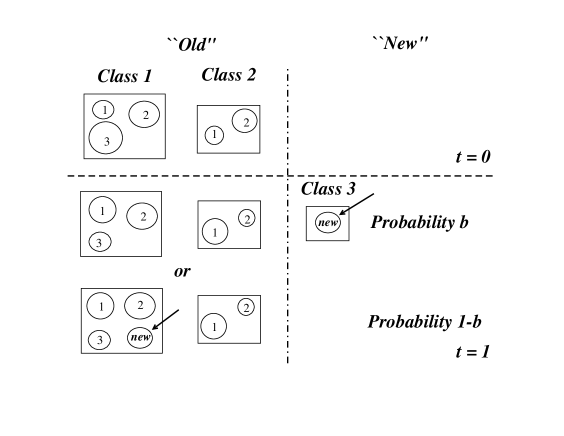
Figure 1: Schematic representation of the model of proportional growth. At time $t=0$, there are $N(0)=2$ classes ($\square$) and $n(0)=5$ units ($\bigcirc$) (Assumption A1). The area of each circle is proportional to the size $\xi$ of the unit, and the size of each class is the sum of the areas of its constituent units (see Assumption B1). At the next time step, $t=1$, a new unit is created (Assumption A2). With probability $b$ the new unit is assigned to a new class (class 3 in this example) (Assumption A3). With probability $1-b$ the new unit is assigned to an existing class with probability proportional to the number of units in the class (Assumption A4). In this example, a new unit is assigned to class $1$ with probability $3/5$ or to class $2$ with probability $2/5$. Finally, at each time step, each circle $i$ grows or shrinks by a random factor $\eta_{i}$ (Assumption B2).

We model business firms as classes consisting of a random number of units. According to this view, a firm is represented as the aggregation of its constituent units such as divisions (Amaral98, ), businesses (Sutton02, ), or products (DeFabritiis03, ). We study the logarithm of the one-year growth rate of classes $g\equiv\log(S(t+1)/S(t))$ where $S(t)$ and $S(t+1)$ are the sizes of classes in the year $t$ and $t+1$ measured in monetary values (GDP for countries, sales for firms and products). The model is illustrated in Fig. 1. The model is built upon two key sets of assumptions:

• the number of units in a class grows in proportion to the existing number of units;

• the size of each unit grows in proportion to its size.

More specifically, the first set of assumptions is:

1. Each class $\alpha$ consists of $K_{\alpha}(t)$ number of units. At time $t=0$, there are $N(0)$ classes consisting of $n(0)$ total number of units.

2. At each time step a new unit is created. Thus the number of units at time $t$ is $n(t)=n(0)+t$.

3. With birth probability $b$, this new unit is assigned to a new class.

4. With probability $1-b$, a new unit is assigned to an existing class $\alpha$ with probability $P_{\alpha}=(1-b)K_{\alpha}(t)/n(t)$.

The second set of assumptions of the model is:

1. At time $t$, each class $\alpha$ has $K_{\alpha}(t)$ units of size $\xi_{i}(t)$, ${i=1,2,...K_{\alpha}(t)}$ where $K_{\alpha}$ and $\xi_{i}>0$ are independent random variables.

2. At time $t+1$, the size of each unit is decreased or increased by a random factor $\eta_{i}(t)>0$ so that

   $$\xi_{i}(t+1)=\xi_{i}(t)\,\eta_{i}(t),$$ (1)

   where $\eta_{i}(t)$, the growth rate of unit $i$, is independent random variable.

Based on the first set of assumptions, we derive $P(K)$, the probability distribution of the number of units in the classes at large $t$. Then, using the second set of assumptions with $P(K)$ we calculate the probability distribution of growth rates $P(g)$. Since the exact analytical solution of $P(K)$ is not known, we provide approximate mean field solution for $P(K)$ (see, e.g., Chapter 6 of (book, )). We also assume that $P(K)$ follows exponential distribution either in old and new classes (Cox, ).

Therefore, the distribution of units in all classes is given by

$$P(K)=\frac{N(0)}{N(0)+bt}\,P_{old}(K)\,+\,\frac{bt}{N(0)+bt}\,P_{new}(K).$$ (2)

where $P_{old}(K)$ and $P_{new}(K)$ are the distribution of units in pre-existing and new classes, respectively.

Let us assume both the size and growth of units ($\xi_{i}$ and $\eta_{i}$ respectively) are distributed as $LN(m_{\xi},V_{\xi})$ and $LN(m_{\eta},V_{\eta})$ where $LN$ means lognormal distribution. Thus, for large $K$, $g$ has a Gaussian distribution

$$P(g|K)={\frac{\sqrt{K}}{\sqrt{2\pi V}}}\,\exp\left(-\frac{(g-m)^{2}K}{2V}\right),$$ (3)

where $m$ is the function of $m_{\eta}$ and $V_{\eta}$, and $V$ is the function of $V_{\xi}$ and $V_{\eta}$. Thus, the resulting distribution of the growth rates of all classes is determined by

$$P(g)\equiv\sum_{K=1}^{\infty}P(K)P(g|K).$$ (4)

The approximate solution of $P(g)$ is obtained by using Eq. (3) for $P(g|K)$ for finite $K$, mean field solution Eq. (2) for $P(K)$ and replacing summation by integration in Eq. (4). After some algebra, we find that the the shape of $P(g)$ based on either $P_{old}(K)$ or $P_{new}(K)$ is same, and $P(g)$ is given as follows

$$P(g)\approx\frac{2V}{\sqrt{g^{2}+2V}\,(|g|+\sqrt{g^{2}+2V})^{2}}.$$ (5)

which behaves for $g\to 0$ as $1/\sqrt{2V}-|g|/V$ and for $g\to\infty$ as $V/(2g^{3})$. Thus, the distribution is well approximated by a Laplace distribution in the body with power-law tails.

3 The Empirical Evidence

We analyze different levels of aggregation of economic systems, from the micro level of products to the macro level of industrial sectors and national economies.

We study a unique database, the pharmaceutical industry database (PHID), which records sales figures of the $189,303$ products commercialized by $7,184$ pharmaceutical firms in $21$ countries from 1994 to 2004, covering the whole size distribution for products and firms and monitoring the flows of entry and exit at both levels. Moreover, we investigate the growth rates of all U.S. publicly-traded firms from 1973 to 2004 in all industries, based on Security Exchange Commission filings (Compustat). Finally, at the macro level, we study the growth rates of the gross domestic product (GDP) of $195$ countries from 1960 to 2004 (World Bank).

Figure 2a shows that the growth distributions of countries, firms, and products seems quite different but in Fig. 2b they are all well fitted by Eq. (5) just with different values of $V$. Growth distributions at any level of aggregation depict marked departures from a Gaussian shape. Moreover, while the $P(g)$ of GDP can be approximated by a Laplace distribution, the $P(g)$ of firms and products are clearly more leptokurtic than Laplace. Coherently with the predictions of the model outlined in Section 2, we find that both product and firm growth distributions are Laplace in the body (Fig. 3), with power-law tails with an exponent $\zeta=3$ (Fig. 4).

4 Discussion

We introduce a simple and general model that accounts for both the central part and the tails of growth distributions at different levels of aggregation in economic systems. In particular, we show that the shape of the business firm growth distribution can be accounted for by a simple model of proportional growth in both number and size of their constituent units. The tails of growth rate distributions are populated by younger and smaller firms composed of one or few products while the center of the distribution is shaped by big multi-product firms. Our model predicts that the growth distribution is Laplace in the central part and depicts an asymptotic power-law behavior in the tails. We find that the model’s predictions are accurate.

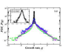
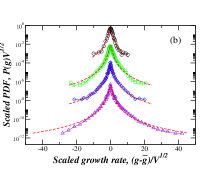
Figure 2: (a) Empirical results of the probability density function (PDF) $P(g)$ of growth rates. Shown are country GDP ($\bigcirc$), pharmaceutical firms ($\square$), manufacturing firms ($\Diamond$), and pharmaceutical products ($\bigtriangleup$). (b) Empirical tests of Eq. (5) for the probability density function (PDF) $P(g)$ of growth rates rescaled by $\sqrt{V}$. Dashed lines are obtained based on Eq. (5) with $V\approx 4\times 10^{-4}$ for GDP, $V\approx 0.014$ for pharmaceutical firms, $V\approx 0.019$ for manufacturing firms, and $V\approx 0.01$ for products. After rescaling, the four PDFs can be fit by the same function. For clarity, the pharmaceutical firms are offset by a factor of $10^{2}$, manufacturing firms by a factor of $10^{4}$ and the pharmaceutical products by a factor of $10^{6}$.

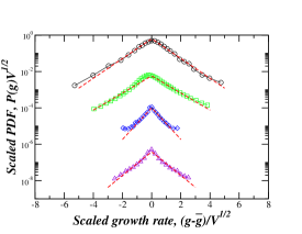
Figure 3: Empirical tests of Eq. (5) for the central part in the PDF $P(g)$ of growth rates rescaled by $\sqrt{V}$. Shown are 4 symbols: country GDP ($\bigcirc$), pharmaceutical firms ($\square$), manufacturing firms ($\Diamond$), and pharmaceutical products ($\bigtriangleup$). The shape of central parts for all four levels of aggregation can be well fit by a Laplace distribution (dashed lines). Note that Laplace distribution can fit $P(g)$ only over a restricted range, from $P(g)=1$ to $P(g)\approx 10^{-1}$.

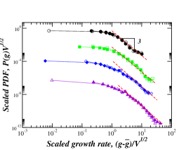
Figure 4: Empirical tests of Eq. (5) for the tail parts of the PDF of growth rates rescaled by $\sqrt{V}$. The asymptotic behavior of $g$ at any level of aggregation can be well approximated by power laws with exponents $\zeta\approx 3$ (dashed lines). The symbols are as follows: Country GDP (left tail: $\bigcirc$, right tail: $\bullet$), pharmaceutical firms (left tail: $\square$, right tail: $\blacksquare$), manufacturing firms (left tail: $\Diamond$, right tail: $\blacklozenge$), pharmaceutical products (left tail: $\bigtriangleup$, right tail: $\blacktriangle$).

References

- (1) Gibrat, R. (1931) Les Inégalités Économiques (Librairie du Recueil Sirey, Paris).
- (2) Kapteyn, J. & Uven M. J. (1916) Skew Frequency Curves in Biology and Statistics (Hoitsema Brothers, Groningen).
- (3) Zipf, G. (1949) Human Behavior and the Principle of Least Effort (Addison-Wesley, Cambridge, MA).
- (4) Gabaix, X. (1999) Quar. J. Econ. 114, 739–767.
- (5) Steindl, J. (1965) Random Processes and the Growth of Firms: A study of the Pareto law (London, Griffin).
- (6) Sutton, J. (1997) J. Econ. Lit. 35, 40-59.
- (7) Kalecki, M. (1945) Econometrica 13, 161-170.
- (8) Simon, H. A. (1955) Biometrika, 42, 425-440.
- (9) Ijiri, Y. & Simon, H. A., (1977) Skew distributions and the sizes of business firms (North-Holland Pub. Co., Amsterdam).
- (10) Stanley, M. H. R., Amaral, L. A. N., Buldyrev, S. V., Havlin, S., Leschhorn, H., Maass, P., Salinger, M. A. & Stanley, H. E. (1996) Nature 379, 804-806.
- (11) Lee, Y., Amaral, L. A. N., Canning, D., Meyer, M. & Stanley, H. E. (1998) Phys. Rev. Lett. 81, 3275-3278.
- (12) Plerou, V., Amaral, L. A. N., Gopikrishnan, P., Meyer, M. & Stanley, H. E. (1999) Nature 433, 433-437.
- (13) Bottazzi, G., Dosi, G., Lippi, M., Pammolli, F. & Riccaboni, M. (2001) Int. J. Ind. Org. 19, 1161-1187.
- (14) Matia, K., Fu, D., Buldyrev, S. V., Pammolli, F., Riccaboni, M. & Stanley, H. E. (2004) Europhys. Lett. 67, 498-503.
- (15) Fu, D., Pammolli, F., Buldyrev, S.V., Riccaboni, M., Matia, K., Yamasaki, K., Stanley, H.E. (2005) PNAS 102, 18801–18806.
- (16) Amaral, L. A. N., Buldyrev, S. V., Havlin, S., Leschhorn, H, Maass, P., Salinger, M. A., Stanley, H. E. & Stanley, M. H. R. (1997) J. Phys. I France 7, 621–633.
- (17) Buldyrev, S. V., Amaral, L. A. N., Havlin, S., Leschhorn, H, Maass, P., Salinger, M. A. , Stanley, H. E. & Stanley, M. H. R. (1997) J. Phys. I France 7, 635–650.
- (18) Sutton, J. (2002) Physica A 312, 577–590.
- (19) Fabritiis, G. D., Pammolli, F. & Riccaboni, M. (2003) Physica A 324, 38–44.
- (20) Amaral, L. A. N., Buldyrev, S. V., Havlin, S., Salinger, M. A. & Stanley, H. E. (1998) Phys. Rev. Lett 80, 1385–1388.
- (21) Takayasu, H. & Okuyama, K. (1998) Fractals 6, 67–79.
- (22) Canning, D., Amaral, L. A. N., Lee, Y., Meyer, M. & Stanley, H. E. (1998) Econ. Lett. 60, 335–341.
- (23) Buldyrev, S. V., Dokholyan, N. V., Erramilli, S., Hong, M., Kim, J. Y., Malescio, G. & Stanley, H. E. (2003) Physica A 330, 653–659.
- (24) Kalecki, M. R. Econometrica (1945) 13, 161–170.
- (25) Reed, W. J. (2001) Econ. Lett. 74, 15–19.
- (26) Stanley, H. E. (1971) Introduction to Phase Transitions and Critical Phenomena (Oxford University Press, Oxford).
- (27) Cox, D. R. & Miller, H. D. (1968) The Theory of Stochastic Processes (Chapman and Hall, London).
- (28) Kotz, S., Kozubowski, T. J. & Podgórski, K. (2001) The Laplace Distribution and Generalizations: A Revisit with Applications to Communications, Economics, Engineering, and Finance (Birkhauser, Boston).