Directional emission of stadium-shaped micro-lasers

Abstract

The far-field emission of two dimensional (2D) stadium-shaped dielectric cavities is investigated. Micro-lasers with such shape present a highly directional emission. We provide experimental evidence of the dependance of the emission directionality on the shape of the stadium, in good agreement with ray numerical simulations. We develop a simple geometrical optics model which permits to explain analytically main observed features. Wave numerical calculations confirm the results.

The field of quantum chaos has widely broadened over the last two decades ecoles . Generally, it relates the quantum behavior of a broad diversity of systems with their classical features. In this context, lossless billiards are models of great interest, providing a broad variety of dynamical systems by changing the shape of the boundary. Moreover they are accessible to experimental studies microondes ; Davidson . In the same time, the influence of loss or noise on open quantum systems is also being investigated decoherence , with emphasis on the behavior of open quantum systems with chaotic classical dynamics cvitanovic ; boulanger ; random . Flat micro-lasers exhibiting different boundary shapes are relevant examples of open billiards with a coherent output coupling copains .

Here we focus on polymer micro-lasers of the Bunimovich stadium shape. Such billiard is the archetype of chaotic systems bunimovich . Stadium billiards look like a rectangle of length $2l$ between two half-circles of diameter $2r$, accounted the form ratio $l/r$ (see Fig. 1). Though all periodic orbits are unstable, dielectric micro-cavities with this shape are well-behaved lasers with highly directional emission in the far-field pattern APL . Aside from quantum chaos studies, such micro-resonators are also being considered for applications in integrated optics and biological sensors naisbio .

This letter is devoted to the investigation of the directional emission versus the form ratio as a way to infer general behavior for such dynamical systems. First we present experimental results and show a good agreement with ray numerical simulations. Then we develop a simple ray model which permits to describe analytically main observed features. All these results are finally confirmed by electromagnetic numerical calculations.

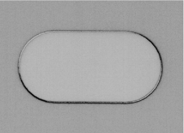
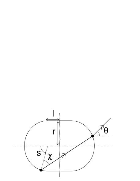
Figure 1: Left: Optical microscope image of a stadium-shaped micro-laser with $l/r=1$ and $r~{}=~{}30~{}\mu m$. Right: Notations. $l$ is the half-length of the rectangle and $r$ is the radius of the half-circles. $s$ is the curvilinear coordinate along the boundary, $\chi$ is the incident angle and $\theta$ is the outgoing angle measured from the main axis of the stadium.

The micro-laser cavities are etched in a thin layer of a passive polymer matrix (PMMA: $polymethyl\-methacrylate$), doped with a guest laser dye (DCM: $4-dicyanomethylene-2-methyl-6-(4-di\-me\-thyl\-amino\-styryl)-4H-pyran$). Our versatile fabrication process ensures for broad variations in size ($r=10~{}\mu m$ to $50~{}\mu m$), shape ($l/r=0$ to $l/r=5$) and thickness (between $0.4~{}\mu m$ and $0.7~{}\mu m$ to avoid vertical multimode behavior) with quality factor $Q$ greater than 6000 APL . The microlasers are pumped uniformly from above at $532~{}nm$ with a frequency doubled picosecond Nd:YAG laser and emit from their sides with $\lambda\simeq 600~{}nm$. Such 2D dielectric billiards present an effective refractive index $n$ of 1.5 and are operating in the semi-classical regime ($r/\lambda$ varying from typically $20$ up to $100$). The emitted light is collected in the far-field and coupled to a multi-channel detector via a spectrometer. A typical experimental spectrum is shown in Fig. 2 (bottom). The sample is fixed on a rotating mount and the intensity emitted in a given direction is obtained by summing over all pixels of the spectrum. Far-field spectra are performed over 360^∘ by 5^∘ steps with the aperture angle of about 15^∘.

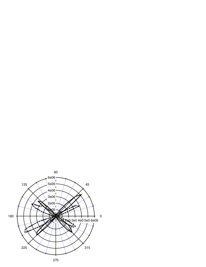
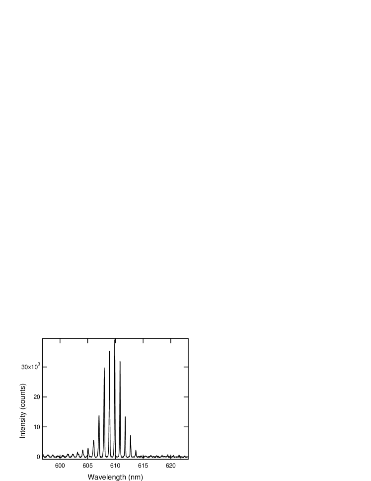
Figure 2: Top: Experimental far-field emission in the plane of a 2D stadium-shaped micro-laser as a function of the polar angle for $l/r=0.5$ (solid line) and $l/r=1$ (dashed line). Bottom: Experimental far-field spectrum for $l/r=2$ and $r=17.5~{}\mu m$.

The intensity of the laser emission versus the $\theta$ angle (see Fig. 1 (right) for notations) is displayed in Fig. 2 (top). The emission exhibits a high directionality along four directions, symmetrical with respect to the 0^∘ and 90^∘ axis, according to the obvious symmetries of the stadium shape. The direction of maximal emission depends on the $l/r$ form ratio. Experimental results are summarized in Fig. 3 for form ratios ranging from $l/r=0.5$ to $l/r=3$. They represent an optimum for reproducibility according to our 5^∘ precision interval.

Even if stadium-shaped billiards are fully chaotic systems, these micro-lasers present experimentally a highly directional emission in the far-field pattern. The direction of maximal emission depends on the $l/r$ form ratio and a variation of more than 30^∘ has been measured between $l/r=0.5$ and $l/r=3$ (Fig. 3)what can be of great interest for applications in integrated optics.

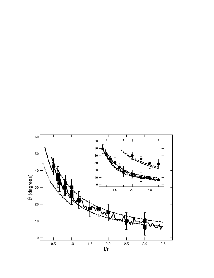
Figure 3: Direction of maximal emission $\theta$ versus form ratio $l/r$. Squares represent experimental results. Solid line indicates dominant contribution of ray numerical simulations and dotted line is the position of the largest satellite peak. Dashed lines are lens model predictions (2) with $m=0$ (lower line) and $m=-1$ (upper line). Inset: Comparison of ray (solid line) and wave numerical simulations (circles). Dashed lines are lens model predictions with (from bottom to top) $m=0,-1,1,-2$.

To account for these experimental results, we first perform usual ray numerical simulations consisting in probing a large number of randomly defined rays ($\sim 10^{7}$) with starting points and initial directions uniformly distributed over the whole phase space. Each ray propagates along a straight line and is totally reflected at the boundary until the incident angle $\chi$ becomes smaller than the critical angle, $\chi_{c}=\mathrm{arcsin}(1/n)$, thus allowing the ray to escape by refraction . The stadium-shaped billiard is fully chaotic, so almost each ray escapes after propagating over a finite distance. Typical histograms of the outgoing angles are plotted in Fig. 4.

Figure 4: Histograms of outgoing angles obtained by ray numerical simulations with threshold equal twice the billiard perimeter for $l/r=0.5$ (solid line), $l/r=1$ (dotted line), and $l/r=2.5$ (dashed line). Pictures normalized to unit maximum. Inset: The same for $l/r=0.5$ but without cut off.

To remove the background, only those rays which propagate over more than a finite threshold distance (twice the billiard perimeter in Fig. 4) are taken into account. Histograms are indented by peaks which reveal the structure of underlying unstable manifolds josab ; prlharayama . An histogram is calculated for each form ratio value and the position of its maximum is plotted versus $l/r$ in Fig. 3 (solid lines). The plot is in excellent agreement with real experimental results as seen from Fig. 3.

For some $l/r$ values ray simulations reveal the existence of a few peaks with comparable amplitudes (cf. Fig. 4). Dotted line branch in Fig. 3 indicates the most prominent satellite peak. Nevertheless dominant experiment contribution is assumed to correspond to the upper branch because its associated intensity (integral below the peak) is larger than the other one (cf. solid line curve in Fig. 4).

To explain main features of experiments and ray simulations, we develop a simple model based on geometrical optics. To minimize refraction loss, rays propagating near the boundary are privileged. So we focus on rays which, after being totally reflected on the left half-circle, come to bounce on the right one (see Fig. 1). Long-lived trajectories can be characterized by their density on the Poincaré surface of section with coordinates $s$ and $\sin\chi$. Our main assumption is that this density is uniform in the allowed part of phase-space

$$P(s,\sin\chi)\sim\Theta(\frac{\pi}{2}r-|s|)\Theta(|\sin\chi|-1/n)$$ (1)

where $\Theta(x)$ is the Heaviside step function.

Long-lived trajectories in open chaotic systems are concentrated near unstable manifolds of confined periodic orbits josab ; boulanger . So the true density is a fractal whose correct determination requires the knowledge of large number of periodic orbits. However, finite experimental resolution and quantum effects will smooth out small details and as the first approximation the assumption (1) looks quite natural. Below we show that it leads to simple analytical formulas in a good agreement with direct ray simulations.

Let us consider point sources on the left half-circle emitting light according to (1). Among these, some rays escape by refraction on the right half-circle and one can deduce the histogram of outgoing angles. The dependence of the histogram maximum on $l/r$ reproduces well experiments and ray simulations, validating the assumptions. As the resulting curves are closed to lens model predictions (see below) we did not present them.

To further simplify this approach, we consider the right half-circle as an ideal lens. In this approximation all rays emitted from a point source are focused exactly as rays close to the line connecting the source and the center of the right half-circle (i.e. spherical aberrations are ignored). So the direction of emission $\theta$ corresponds mainly to this line and can be calculated analytically from purely geometrical considerations. It depends on the emission angle $\chi$ and on the number $|m|$ of rebounds on straight boundaries ($m>0$ - resp. $m<0$ - means first bounce on the high - resp. low - straight boundary):

$$\theta(\chi)=|\arcsin\frac{m}{\sqrt{m^{2}+(l/r)^{2}}}+\arcsin\frac{\sin\chi}{2\sqrt{m^{2}+(l/r)^{2}}}\;|.$$

This line exists provided $x_{1}<\sin\chi<x_{2}$ where $x_{1}=1/n$ and $x_{2}=2l/\sqrt{4l^{2}+(2m+1)^{2}r^{2}}$. Formally the channel with given $m$ is open when $x_{1}<x_{2}$ or $l/r>|2m+1|/2\sqrt{n^{2}-1}$ but it may exist for smaller $l/r$ as well. For a given $l/r$, the mean emission angle, $\tilde{\theta}$, is deduced by averaging over the above interval

$$\tilde{\theta}=\frac{1}{x_{2}-x_{1}}\int_{x_{1}}^{x_{2}}\theta(\chi){\rm d}\sin\chi\;.$$ (2)

Within the lens model the emission intensity is proportional to the angle with which the right half-circle is visible from a source point. Direct geometrical calculations show that the dominant contribution for $l/r<3.5$ corresponds to $m=0$ channel. Channel with $m=-1$ has smaller but comparable intensity. Considering experimental precision, other channels can be ignored but they are visible in ray simulations (cf. a small peak around $30^{\circ}$ in the histogram for $l/r=2.5$ in Fig. 4). The directional emission predictions for channels with $m=0$ and $m=-1$ are indicated by dashed lines in Fig. 3. The excellent agreement between these curves, experiments and direct ray simulations confirms that the assumption (1) is relevant to interpret analytically the emission of the stadium-shaped cavity in the geometrical optics domain.

For completeness we perform also numerical calculations in the wave domain. In the simplest approximation, the electromagnetic field is evolving in a passive cavity with a defined polarization. In this case, the electric field (TM polarization) or its magnetic counterpart (TE polarization) is represented by a scalar wave function $\psi$ obeying the two dimensional Helmholtz equation [$(\Delta+n_{i,e}^{2}k^{2})~{}\psi=0$ where refractive index $n_{i}=n$ inside and $n_{e}=1$ outside the cavity] with specific boundary conditions (see e.g. naisbio ). To find eigenvalues $\{k_{m}\}$ and eigenfunctions $\{\psi_{m}\}$ of quasi-stationary states we use the standard boundary element method wiersig . In this approach the wave functions inside and outside the cavity $\psi_{i,e}$ are expressed in terms of single layer potentials $\mu_{i,e}$:

$$\psi_{i,e}(\vec{r}\,)=\oint{\rm d}s~{}\mu_{i,e}(s)~{}H_{0}^{(1)}(kn_{i,e}|\vec{r}-\vec{r}_{s}|)$$ (3)

$s$ is the curvilinear coordinate along the boundary. Here $H_{0}^{(1)}$ is the Hankel function of the first kind. The choice of this Hankel function outside the cavity is dictated by outgoing conditions to infinity

$$\psi_{e}(r,\theta)\stackrel{{\scriptstyle r\to\infty}}{{\longrightarrow}}\frac{{\rm e}^{{\rm i}kr}}{\sqrt{kr}}f(\theta)$$ (4)

and inside the cavity by stability of numerical algorithm.

Following natural filtering by the lasing effect, only modes with small losses are considered, i.e. modes with an imaginary part of the wave-number closed to zero. Most of the well-confined wave-functions present a clear directional emission in the far-field pattern, even for low $|kr|$ (see Fig. 5 (right)). Then it is possible to find positions of directional dominant peaks for each $l/r$ and different eigenvalues which are plotted in Fig. 3 (inset). Each point at fixed $l/r$ corresponds to the averaging of maximal emission angles over a representative set of well-confined eigenfunctions. The error bars corresponds to the mean standard deviation. As was predicted, dominant emission direction corresponds to $m=0$ and $m=-1$ channels of the lens model. It is interesting to notice that channels with $m=1$ and $m=-2$ are also well visible.

So good agreement between geometrical and wave optics does not usually appear for closed chaotic systems. The emission directions of these quantum dielectric billiards behave largely as if they were classical ones, governed by geometrical optics rules. However there is no loss of coherence as in open systems generally studied in the field of decoherence decoherence : experimental spectra present clear peaks (see fig. 2 (bottom)) and no noise is introduced to couple light with the outside of the cavity. Actually the typical distance $L/r$ covered by a photon - of the order of $2Q/n|k|r$ - ranges between 16 and 80 in our experiments. This magnitude suggests that interference effects should be taken into account whereas we have demonstrated that a geometrical optics approach is sufficient to predict the overall directional emission. The lens model shows that it is mostly connected with the existence of only a small number of well defined open emission channels. Under higher precision calculations and experiments, each channel should split into many narrow peaks and quantum phenomena should be more important.

Figure 5: Left: Imaginary part of quasi-stationary eigenvalues versus their real part. These eigenvalues correspond to solutions of the Helmholtz equation with TM boundary conditions for dielectric stadium with $l/r=2$ and refractive index n=1.5 antisymmetric with respect to both axes. Right: Far-field emission pattern of eigenfunctions: $|f(\theta)|^{2}$ in (4) normalized to unit maximum. From top to bottom ($l/r$=0.3, $Re(kr)$=39.31) ; ($l/r$=1, $Re(kr)$=13.88) ; ($l/r$=2, $Re(kr)$=23.29).

In summary, we present experimental results about directional emission of stadium-shaped micro-lasers and demonstrate that they are well described by simple geometrical optics approaches. We develop a lens model which predicts analytically main features of directional emission. Moreover we point out that well-confined wave-functions show a good agreement with these classical predictions while coherent properties are not destroyed.

These kinds of predictions seem to be applicable to a more general class of chaotic dielectric billiards. Experiments and calculations are thus under progress to explore other micro-cavity shapes like cut disk and cardioid.

The authors are grateful to R. Hierle, D. Wright and S. Brasselet for experimental and technological support and to O. Bohigas and T. Nguyen for helpful discussions.

References

- (1) Chaos and Quantum Physics, Proceeding of the 1989 Les Houches Summer School, edited by M. J. Giannoni, A. Voros, and J. Zinn-Justin (Elsevier, 1991); New Directions in Quantum Chaos, Proceedings of the 1999 Varenna Summer School, edited by G. Casati, I. Guarneri, and U. Smilansky (IOS Press, 2000).
- (2) J. Stein, H.-J. Stöckmann, and U. Stoffregen, Phys. Rev. Lett., 75, 53 (1995); H. Alt, C. Dembowski, H.-D. Gräf, R. Hofferbert, H. Rehfeld, A. Richter, and C. Schmit, Phys. Rev. E, 60, 2851 (1999).
- (3) M. F. Andersen, A. Kaplan, and N. Davidson, Phys. Rev. Lett., 90, 023001 (2003).
- (4) S. Habib, K. Shizume, and W. H. Zurek, Phys. Rev. Lett., 80, 4361, (1998).
- (5) P. Cvitanovic and B. Eckhardt, Phys. Rev. Lett., 63, 823 (1989); K. Pance, W. Lu, and S. Sridhar, Phys. Rev. Lett., 85, (13), 2737 (2000).
- (6) J.P. Keating, M. Novaes, S.D. Prado, and M. Sieber, quant-ph/0605217; S. Nonnenmacher and M. Rubin, in preparation.
- (7) X. Jiang, S. Feng, C. M. Soukoulis, J. Zi, J. D. Joannopoulos, and H. Cao, Phys. Rev. B, 69, 104204 , (2004).
- (8) C. Gmachl, F. Capasso, E. E. Narimanov, J. U. Nöckel, A. D. Stone, J. Faist, D. L. Sivco, and A. Y. Cho, Science, 280, 1556 (1998); T. Harayama, P. Davis, and K. S. Ikeda, Phys. Rev. Lett., 90, 063901, (2003); A. D. Stone, Physics Today, 58, (8), 37 (2005).
- (9) L. A. Bunimovich, Commun. Math. Phys., 65, 295 (1979).
- (10) M. Lebental, J.-S. Lauret, R. Hierle, and J. Zyss, Appl. Phys. Lett., 88, 031108 (2006).
- (11) Proceedings of the International School of Quantum Electronics, edited by F. Michelotti, A. Driessen, M. Bertolotti, AIP conference proceedings, 709 (2004).
- (12) H. G. L. Schwefel, N. B. Rex, H. E. Tureci, R. K. Chang, A. D. Stone, T. Ben-Messaoud and J. Zyss, Jour. Opt. Soc. Am. B , 21, 923 (2004).
- (13) S. Shinohara, T. Harayama, H. E. Tureci and A. D. Stone, physics/0606212.
- (14) J. Wiersig, Phys. Rev. A, 67, 023807 (2003).