Dynamics of the Warsaw Stock Exchange index as analysed by the nonhomogeneous fractional relaxation equation

Abstract

We analyse the dynamics of the Warsaw Stock Exchange index WIG at a daily time horizon before and after its well defined local maxima of the cusp-like shape decorated with oscillations. The rising and falling paths of the index peaks can be described by the Mittag-Leffler function superposed with various types of oscillations. The latter is a solution of our model of index dynamics defined by the nonhomogeneous fractional relaxation equation. This solution is a generalised analog of an exactly solvable model of viscoelastic materials. We found that the Warsaw Stock Exchange can be considered as an intermediate system lying between two complex ones, defined by short and long-time limits of the Mittag-Leffler function; these limits are given by the Kohlraush-Williams-Watts law for the initial times, and the power-law or the Nutting law for asymptotic time. Hence follows the corresponding short- and long-time power-law behaviour (different ”universality classes”) of the time-derivative of the logarithm of WIG which can in fact be viewed as the ”finger print” of a dynamical critical phenomenon.

05.45.Tp, 89.65.Gh, 89.75.-k

1 Introduction

It seems that there are many distinct analogies between the dynamics and/or stochastics of complex physical and economical or even social systems [1, 2, 3, 4, 5, 6, 7, 8, 9]. The methods and even algorithms that have been explored for description of physical phenomena become an effective background and inspiration for very productive methods used in analysis of economical data [10, 11].

In this paper we study an emerging market and more precisely, the historical Warsaw Stock Exchange (WSE) index WIG at a daily time horizon at the closing; we think that its dynamics is typical for an emerging financial market of small and moderate size. Our concept is to consider only well developed temporal (local) maxima of the cusp-like shape decorated with some oscillations (cf. peaks denoted by $A,a,B,C$ in Fig.1) which cover the greater part of the whole time series. Our goal is to describe the slowing down of rising and relaxation processes within these temporal maxima by assuming a retarded feedback as a principal effect (except the rising path within the first local peak which, in principle, is exponential; cf. Fig.2). This feedback is a reminiscence of investors’ activity stimulated mainly by their observations of the empirical data in the past.

1.1 Inspiration

Our analysis was inspired by the non-Debye or non-exponential, fractional relaxation processes observed, for example, in stress-strain relaxation present in viscoelastic materials [19, 13, 14]. The most commonly used empirical decay function for handling non-Debye relaxation processes in complex systems are described either by a Kohlraush-Williams-Watts (KWW) or a stretched exponential decay function [15] for short time-range $t\ll\tau$:

$$f(t)\sim\exp\left(-\left(\frac{t}{\tau}\right)^{\alpha}\right),$$ (1)

where $0<\alpha<1$, or by an asymptotic power-law (Nuttig law) for $t\gg\tau$:

$$f(t)\sim\left(\frac{t}{\tau}\right)^{-\alpha}.$$ (2)

From expressions (1) and (2) we obtain for the change of $\ln f(t)$ per unit time

$$\frac{d\ln f(t)}{dt}\sim\left\{\begin{array}[]{cc}\frac{1}{t^{1-\alpha}}&\mbox{for $t\ll\tau$}\\ \frac{1}{t}&\mbox{for $t\gg\tau$},\end{array}\right.$$ (5)

which defines the power-law limits of the dynamics, i.e. it defines (for $t\ll\tau$) a universality class (characterized by dynamical, critical exponent $1-\alpha$) which, in fact, can be viewed as the ”finger print” of a dynamical critical phenomenon. For such a peak the derivative diverges at the extremal point (i.e. at $t=0$) which justifies the name ”sharp peak” used often in the literature in this context (cf. [6] and refs. therein). For a sufficiently wide empirical window it would be possible to observe a transition from the KWW to the Nutting behaviour and from one kind of power-law to another, correspondingly.

Note that the non-exponential relaxation introduces memory, i.e. the underlying fundamental processes are of non-Markovian type. It was shown that a natural way to incorporate memory effects is fractional calculus. The power-law kernel defining the fractional relaxation equation involves a particularly long memory. The function which plays a dominating role in fractional relaxation problems is indeed the Mittag-Leffler (ML) function [16]

$$E_{\alpha}\left(-\left(\frac{t}{\tau}\right)^{\alpha}\right)=\sum_{n=0}^{\infty}\frac{(-(t/\tau)^{\alpha})^{n}}{\Gamma(1+\alpha n)},$$ (6)

which is a natural generalisation of the exponential one. This function interpolates between cases (1) and (2) and plays a central role in our analysis.

2 The model

Our phenomenological model of index dynamics consists of two stages:

• Formulation of a linear ordinary differential equation of the first order with no feedback incorporated which describes evolution of an auxiliary, synthetic index only.

• A conjecture which transforms the above mentioned equation to a more general fractional form which already models the evolution of the empirical Warsaw Stock Exchange index.

Figure 1: The daily closing value of the Warsaw Stock Exchange index WIG (measured by conventional points (p)) from April 16, 1991 (the beginning of the Warsaw Stock Exchange activity) to the $30^{th}$ of March 2006; the presented time series consists of empirical data points for $3382$ trading days (td). The local maxima denoted as $A,\;a,\;B$ and $C$ are analysed further in the text.

The transition from (i) to (ii) means that the system is changed from an unrealistic to a realistic, complex one where the retarded feedback plays an essential role. By using this model we are able to describe the well developed temporal maxima present in daily time series defined by WIG activity (cf. four maxima $A,\;a,\;B$ and $C$ shown in Fig.1).

2.1 Evolution of WIG

The time-dependent value of WIG, $X(t)$, can be decomposed into two components which are recorded and can be even electronically accessible for traders:

• The instantaneous offset $U(t)\stackrel{{\scriptstyle\rm def.}}{{=}}U_{+}(t)-U_{-}(t)$ between the temporal (total) demand $U_{+}(t)\geq 0$ for stocks defining WIG and their (total) temporal supply $U_{-}(t)\geq 0$.

• The instantaneous volume trade $V(t)\stackrel{{\scriptstyle\rm def.}}{{=}}min[U_{+}(t),U_{-}(t)]$ of stocks of the companies which consitute WIG.

Hence, we can write the following instantaneous superposition

$$X(t)=A\cdot U(t)+B\cdot V(t),$$ (7)

where $A(>0)$ and $B$ are referred to as coefficients of relocation. Note that paradoxally index $X(t)$ can change even when the volume of trade, $V(t)$, vanishes, i.e. when the demand or supply vanishes. On the other hand, for vanishing $U(t)$ (when the demand is balanced by the supply) volume trade, $V(t)$, can be still nonvanishing which leads to the change of WIG.

To consider the dynamics (evolution) of WIG, we complete eq.(7) by the differential one which exhibits an instantaneous, therefore unrealistic, feedback to the financial market, namely

$$\frac{dV(t)}{dt}=C\cdot V(t)+D\cdot X(t)+E\cdot\frac{dX(t)}{dt},$$ (8)

where coefficients $C,\;D$ are rates while $E$ is again a kind of relocation coefficient. By combining eqs.(7) and (8) we eliminate the $V(t)$ variable and obtain (after integration),

$$X(t)-X(0)-sgn(C^{\prime})\;\tau_{1}^{-1}\;{}_{0}D_{t}^{-1}X(t) = -A^{\prime}\;sgn(C)\;\tau_{0}^{-1}\;{}_{0}D_{t}^{-1}U(t)$$ (9)

$$+ A^{\prime}\;[U(t)-U(0)],$$

where the definition of an inverse derivative of the first order was used; the definition of its general $n^{th}$ order version (for $n=1,2,3,\ldots$) has a useful form given by the Cauchy formula of repeated integration

$$\;{}_{0}D_{t}^{-n}f(t) \stackrel{{\scriptstyle\rm df.}}{{=}} \int_{0}^{t}dt_{n-1}\int_{0}^{t_{n-1}}dt_{n-2}\ldots\int_{0}^{t_{1}}f(t_{0})dt_{0}$$ (10)

$$= \frac{1}{\Gamma(n)}\int_{0}^{t}dt^{\prime}(t-t^{\prime})^{n-1}f(t^{\prime}).$$

The combined coefficients

$$A^{\prime}=\frac{A}{1-BE},\;C^{\prime}=C\;\frac{1-B\;\frac{D}{C}}{1-BE},\tau_{0}^{-1}\stackrel{{\scriptstyle\rm df.}}{{=}}\;\mid C\mid,\;\tau_{1}^{-1}\stackrel{{\scriptstyle\rm df.}}{{=}}\;\mid C^{\prime}\mid,$$ (11)

which are valid for $BE\not=1$; otherwise, instead of eq.(9) we would obtain a very special one.

The integral eq.(9) defines the model which is an analog of the Zener one for viscoelastic solids [17] in which the stress ($U$) - strain ($X$) relationship is given originally by the linear first order differential equation [14]. Indeed, eq.(9) is the one which we generalize to the fractional form by applying its Maxwell formulation [18]. This formulation consists of a spring (obeying Hooke’s law) and a dashpot (obeying Newton’s law of viscosity) in series; this arrangement shows a simple spatial separation of the solid (elastic) and the fluid (viscous) aspects and it is too specific to describe real viscoelastic materials. However, the hierarchical arrangement of a number (in general infinite) springs and dashpots is already sufficient [18]. Note, that in our approach the spring defines a purely emotional or irrational investors’ activity while the dashpot defines a purely rational one.

2.2 Conjecture

There are several definitions of fractional differentiation and integration [19]. In what follows we are dealing strictly with the Liouville-Riemann (LR) fractional calculus. The fractional integration of arbitrary order $\alpha(>0)$ of function $f(t)$ is a straightforward generalisation of (10),

$$\;{}_{0}D_{t}^{-\alpha}f(t)\stackrel{{\scriptstyle\rm df.}}{{=}}\frac{1}{\Gamma(\alpha)}\int_{0}^{t}dt^{\prime}\frac{f(t^{\prime})}{(t-t^{\prime})^{1-\alpha}},$$ (12)

where $\;{}_{0}D_{t}^{-\alpha}$ is the LR fractional integral operator of order $\alpha$ [19].

The fractional generalization of eq.(9) is performed by replacing expressions $\tau_{0}^{-1}\;{}_{0}D_{t}^{-1}U(t)$ and $\tau_{1}^{-1}\;{}_{0}D_{t}^{-1}X(t)$ by $\tau_{0}^{-\alpha}\;{}_{0}D_{t}^{-\alpha}U(t)$ and $\tau_{1}^{-\alpha}\;{}_{0}D_{t}^{-\alpha}X(t)$ ones, respectively, where the fractional (in general) exponent $\alpha$ is a free but most important shape parameter. Hence, we obtain the fractional integral equation which is able to describe both independent paths (the rising and relaxation) of local temporary peaks of WIG:

$$X(y)-X(0) = -\tau_{1}^{-\alpha}\;{}_{0}D_{y}^{-\alpha}X(y)-A^{\prime}\;sgn(C)\;\tau_{0}^{-\alpha}\;{}_{0}D_{y}^{-\alpha}U(y)$$ (13)

$$+ A^{\prime}\;[U(y)-U(0)],$$

where it was tacitly assumed that $sgn(C^{\prime})=-1$, while the independent variable

$$y=\left\{\begin{array}[]{cc}t_{MAX}-t&\mbox{for rising: $t\leq t_{MAX}$}\\ t-t_{MAX}&\mbox{for relaxation: $t\geq t_{MAX}$.}\end{array}\right.$$ (16)

As both paths of any peak are assumed as independent ones we consider all parameters present in eq.(13) as (in general) different for different paths.

For relaxation the first term on the rhs of eq.(13) describes feedback where the retarded value of index influences the present one; this value is sensitive here to the past one due to the algebraic, integral kernel. The second term on the rhs of eq.(13) desribes explicitly a financial market retarded influence on the index (or the stock price); the third term gives the instantaneous influence. However, for the rising path the situation is more complicated and eq.(13) constitutes only a formal, convenient way to describe it. As we prove, the first and third terms constitute mainly the basis of a dynamical structure of the local (temporal) maximum of WIG.

2.3 Relaxation and rising fractional differential equations

To make a step towards the interpretation, we define the fractional differentiation of order $\gamma(>0)$

$$\;{}_{0}D_{t}^{\gamma}f(t)\stackrel{{\scriptstyle\rm df.}}{{=}}\frac{d^{n}}{dt^{n}}\left(\;{}_{0}D_{t}^{\gamma-n}f(t)\right),$$ (17)

which is considered to be composed of a fractional integration of the order $\alpha\stackrel{{\scriptstyle\rm def.}}{{=}}n-\gamma\;(-1\leq\gamma-n<0)$ followed by an ordinary differentiation of order $n$. Now, by ordinary differentiation of the first order of eq.(13) and by applying definition (17) we obtain the linear inhomogeneous fractional differential equation

$$\frac{dX(y)}{dy} = -\tau_{1}^{-\alpha}\;{}_{0}D_{y}^{1-\alpha}X(y)-A^{\prime}\;sgn(C)\;\tau_{0}^{-\alpha}\;{}_{0}D_{y}^{1-\alpha}U(y)$$ (18)

$$+ A^{\prime}\;\frac{dU(y)}{dy},$$

which describes well both paths of the studied peaks.

2.3.1 Free fractional relaxation: the reference case

We found that the well developed local maxima of the index can be fitted (except for the left-hand side of the first one and up to their oscillations and fluctuations) by an intermediate part of the ML function. In our case we obtained several values of exponent $\alpha$ for WIG’s maxima and almost all of them (except one) are smaller than $0.5$; note that the left-hand side of the first maximum is well fitted by the usual exponential function (or by assuming $\alpha=1$ in the MF function).

In other words, the relaxation of almost all WIG local maxima can be described by the fractional relaxation equation by setting in eq.(18) coefficient $A^{\prime}=0$. Such a simplified equation is, of course, a fractional generalization of the standard relaxation equation whose solution has indeed the form (6) (where variable $t$ is replaced by $y$ and parameter $\tau$ by corresponding $\tau_{1}$ one). This solution is considered here only as a reference case.

2.4 Full Solution of the Fractional Initial Value Problem

We solve the fractional initial value problem (18) by assuming that

$$U(y)=\frac{U(0)}{2}\;[\exp(\imath\;(\omega-\Delta\omega)\;y)+\exp(\imath\;(\omega+\Delta\omega)\;y)],$$ (19)

(where parameters $U(0),\omega,\Delta\omega>0$) and by applying the Laplace transform of a fractional integral operator. Namely, the Laplace transformation of eq.(13) yields

$$\tilde{X}(s)=A^{\prime}\;\frac{1-sgn(C)\tau_{0}^{-\alpha}s^{-\alpha}}{1+\tau_{1}^{-\alpha}s^{-\alpha}}\;{\tilde{U}(s)}+[X(0)-A^{\prime}\;U(0)]\;\frac{s^{-1}}{1+\tau_{1}^{-\alpha}s^{-\alpha}},$$ (20)

where the Laplace transform of the LR fractional integral operator was applied here. By introducing the Laplace transform of (19) into eq.(20) and by using the inverse Laplace transformation in the time domain we can obtain the real part of the solution. However, to compare the prediction of our model with empirical data it is sufficient to use only the lowest order terms in the exact solution, i.e. it is suficient to use the following approximate solution

$$\Re X(y) \approx \left[X(0)+A^{\prime}\;U(0)\;sgn(C)\left(\frac{\tau_{0}}{\tau_{1}}\right)^{-\alpha}\right]E_{\alpha}\left(-\left(\frac{y}{\tau_{1}}\right)^{\alpha}\right)+$$ (21)

$$- A^{\prime}\;U(0)\;sgn(C)\left(\frac{\tau_{0}}{\tau_{1}}\right)^{-\alpha}\cos(\omega\;y)\cos(\Delta\omega\;y),$$

since the parameters $\omega,\;\Delta\omega$, which additionaly multiply the integral terms, were found to be so small that the integral terms are negligible.

2.5 Comparison with empirical data and discussion

In Figs.2-5 we compared the empirical data defining WIG’s local maxima (denoted as $A,\;a,\;B,$ and $C$ in Fig.1) with the predictions given by formula (21). The monotonic curves (obtained by using only the first term) present free solutions while the oscillating curves (obtained by using the whole expression) the full ones, i.e. the free solutions decorated with mono-frequency oscillations (rising and falling paths of peaks $a$ and $B$, respectively) or wiggles (right-hand paths of peaks $A$ and $a$ as well as left-hand path of peak $B$). The values of the key parameters which we obtained are shown in Tables 1-4.

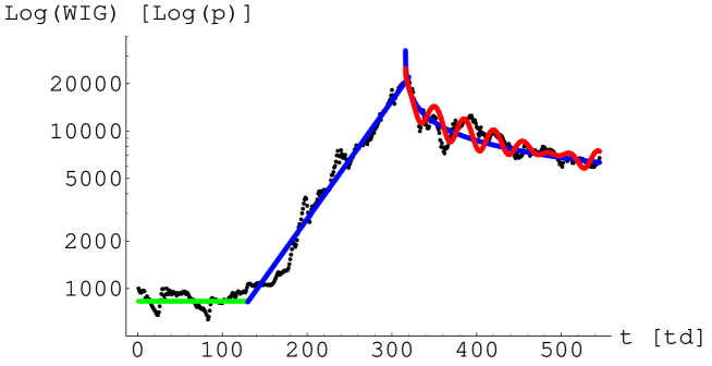
Figure 2: The temporal, local maximum $A$ (cf. Fig.1): the evolution of the daily closing price of WIG in the semi-logarithmic scale (dots) from the beginning of the WSE activity to the end of the first maximum on March 30, 1995; the presented time series consists of data points for $545$ trading days. The tangent solid line was fitted to the left-hand slope of the empirical maximum. The curve fitted to the right-hand slope was obtained by using eq.(21). The values of the corresponding key parameters are presented in Table 1.

Table 1: First set of parameters describing the temporal maximum $A$

Process	$\alpha$	$\tau_{1}\;[td]$	$t_{MAX}\;[td]$	$\omega\;[td^{-1}]$	$\Delta\omega\;[td^{-1}]$
Rising	$1$	$58\pm 1$	$320\pm 1$	$-$	$-$
Relaxation	$0.41$	$176\pm 1$	$316\pm 1$	$0.18$	$0.009$

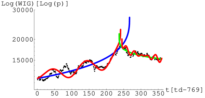
Figure 3: The local maximum $a$ (cf. Fig.1): the evolution of the daily closing value of WIG in the semi-logarithmic scale (dots) dated from the $770^{th}$ trading day (the beginning of this local maximum) to the $1130^{th}$ assumed as the end of this maximum range; the time series consists of data points for $360$ trading days. The curves fitted to left-hand and right-hand paths of the maximum were obtained by using eq.(21); the corresponding key parameters are presented in Table 2.

Table 2: First set of parameters describing the temporal maximum $a$

Process	$\alpha$	$\tau_{1}\;[td]$	$t_{MAX}\;[td]$	$\omega\;[td^{-1}]$	$\Delta\omega\;[td^{-1}]$
Rising	$0.31$	$721.5\pm 1$	$241\pm 1$	$0.063$	$0.005$
Relaxation	$0.25$	$6830\pm 10$	$245\pm 1$	$0.26$	$0.025$

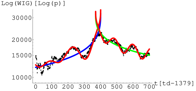
Figure 4: The local maximum $B$ (cf. Fig.1): the evolution of the daily closing value of WIG in the semi-logarithmic scale (dots) dated from the $1380^{th}$ trading day (the beginning of the local maximum) to the $2080^{th}$ day assumed as the end of this maximum range; the presented time series consists of data points for $700$ trading days. The curves fitted to both slopes of the empirical maximum were obtained by using eq.(21). The corresponding key parameters are presented in Table 3.

Table 3: First set of parameters describing the temporal maximum $B$

Process	$\alpha$	$\tau_{1}\;[td]$	$t_{MAX}\;[td]$	$\omega\;[td^{-1}]$	$\Delta\omega\;[td^{-1}]$
Rising	$0.40$	$164\pm 1$	$401\pm 1$	$0.035$	$0.005$
Relaxation	$0.39$	$366.5\pm 1$	$370\pm 1$	$0.055$	$-$

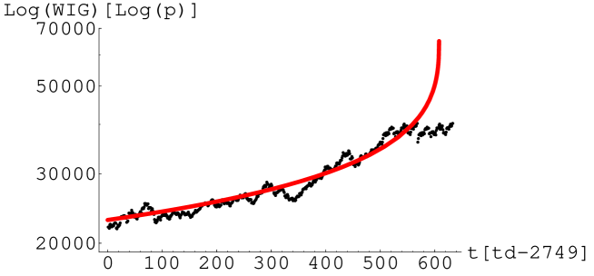
Figure 5: The local maximum $C$ (cf. Fig.1): the evolution of the daily closing value of WIG (dots) dated from the $2750^{th}$ trading day (the beginning of the local maximum) to the $3382^{nd}$ day assumed as the end of the maximum range; the presented time series consists of data points for $633$ trading days. The curve fitted to the left-hand slope of the empirical maximum was obtained by using eq.(21). The corresponding key parameters are presented in Table 4.

Table 4: First set of parameters describing the temporal maximum $C$

Process	$\alpha$	$\tau_{1}\;[td]$	$t_{MAX}\;[td]$
Rising	$0.40$	$249.2\pm 1$	$608\pm 1$

In Fig.6 are presented: (i) the Mittag-Leffler function fitted, for example, to the left-hand path of the empirical maximum $B$ (this is the free solution taken, in fact, from Fig.4), and corresponding (ii) KWW law (lower curve) as well as (iii) the Nutting law (upper curve). This is a typical situation valid both for the left- and right-hand paths of all considered peaks. It is characteristic that none of the peaks reached the fully developed scaling region of the return per unit time $\frac{d\ln X(y)}{dy}$ (cf. section 1.1). In this sense the considered peaks have a precritical character.

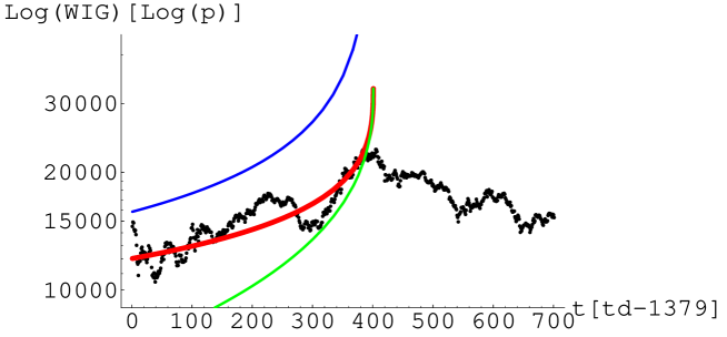
Figure 6: The local WIG’s maximum $B$ (cf. Fig.1): the analysis of the evolution of the daily closing value of the left-hand path presented in the semi-logarithmic scale (dots). The middle solid curve fitted to the left-hand slope of the empirical maximum was taken from Fig.4, while the lower and upper curves are the corresponding limits for the short time given by the streched exponential- or the KWW law (1), and for asymptotic time the power- or the Nutting law is given by (2).

There are several other features common for all peaks which should be noted:

• Both paths of any peak can be considered as independent ones and the location of turning point (extremum) as a random one.

• The considered peaks are asymmetric since:

  • the exponent $\alpha$, which characterizes the left-hand paths of any peak, is larger than the analogous one characterizing the right-hand one,

  • parameter $\tau_{1}$ (defining the time unit) of the left-hand path is smaller than the corresponding one for the right-hand path.

• The location of the extremal point $t_{MAX}$ given by expression (21) is (in general) different for left- and right-hand paths of each peak.

Moreover, a frequency modulation signal is necessary and/or the influence of the signal outside the maximum should be taken into account to describe the beginning of the left-hand paths of peaks $a$ and $B$ (cf. Figs.3 and 4).

Concluding, we suggest that our approach can rationally decrease the risk of investment on the stock market since it is able to warn the investors before the stock market reaches a critical region.

We thank prof. Piotr Jaworski from the Institute of Mathematics at the Warsaw University for his helpful discussion.

References

- [1] R. Badii, A. Politi: Complexity. Hierarchical structures and scaling in physics. Cambridge Univ. Press, Cambridge UK 1997.
- [2] W. Paul, J. Baschnagel: Stochastic Processes. From Physics to Finance. Springer-Verlag, Berlin 1999.
- [3] R.N. Mantegna, H.E. Stanley: An Introduction to Econophysics: Correlations and Complexity in Finance.. CUP, Cambridge UK 2000.
- [4] J.-P. Bouchaud, M. Potters: Theory of Financial Risks. From Statistical Physics to Risk Management. CUP, Cambridhe UK 2001.
- [5] K. Ilinski: Physics of Finance. Gauge modelling in non-equilibrium pricing. J. Wiley & Sons, Chichester 2001.
- [6] B.M. Roehner: Patterns of Speculation. A Study in Observational Econophysics. CUP, Cambridge UK 2002.
- [7] D. Sornette: Why Stock Markets Crash. PUP, Princeton and Oxford 2003.
- [8] Nonextensive statistical mechanics: new trends, new perspectives, Europhysicsnews 36/6 (2005), Special Issue & Directory.
- [9] F. Schweitzer: Brownian Agents and Active Particles. Springer-Verlag, Berlin 2003.
- [10] A. Bunde, J.W. Kantelhardt: Langzeitkorrelationen in der Natur: von Klima, Erbugt und Herzrhythmus. Physikaliche Blätter 57/5 (2001) 49-54.
- [11] D. Grech, Z. Mazur: Statistical Propertiesof Old and New Techniques in Detrended Analysis of Time Series. Acta Phys. Polonica 36/8 (2005) 2403-2413.
- [12] Th.F. Nonnenmacher, R. Metzler: Applications of Fractional Calculus Techniques to Problems in Biophysics in: Applications of Fractional Calculus in Physics. Ed. R. Hilfer. World Sci., Singapore 2000.
- [13] J. Bendler, D.G. LeGrand, W.V. Olszewski: Relaxation and Recovery of Glassy PolyCarbonate in: Transport and Relaxation in Random Materials. Eds. J. Klafter, R.J. Rubin, M.F. Shlasinger, World Sci. Singapore 1986.
- [14] W.G. Glöckle, Th.F. Nonnenmacher: Fractional Integral Operators and Fox Functions in the Theory of Viscoelasticity. Macromolecules 24 (1991)6426-6434.
- [15] R. Richert, A. Blumen: Disordered Systems and Relaxation in: Disorder Effects on Relaxational Processes: Glasses, Polymers, Proteins. Eds. R. Richert, A. Blumen. Springer-Verlag, Berlin 1994.
- [16] R. Metzler, J. Klafter: Tha Random Walk’s Guide to Anomalous Diffusion: A Fractional Dynamics Approach. Phys. Rep. 339 (2000) 1-77.
- [17] N.W. Tschoegel: The Phenomenological Theory of Linear Viscoelastic Behavior. Springer-Verlag, Berlin 1989.
- [18] H. Schiessel and A. Blumen: Hierarchical analogues to fractional relaxation equation. J. Phys. A: Math. Gen 26 (1995) 5057-5069.
- [19] P.L. Butzer, U. Westphal:An Introduction to Fractional Calculus in Fractional Calculus in Physics. Ed. R. Hilfer. World Scient., Singapore 2000.