Variational method for estimating the rate of convergence of Markov Chain Monte Carlo algorithms

Abstract

We demonstrate the use of a variational method to determine a quantitative lower bound on the rate of convergence of Markov Chain Monte Carlo (MCMC) algorithms as a function of the target density and proposal density. The bound relies on approximating the second largest eigenvalue in the spectrum of the MCMC operator using a variational principle and the approach is applicable to problems with continuous state spaces. We apply the method to one dimensional examples with Gaussian and quartic target densities, and we contrast the performance of the Random Walk Metropolis-Hastings (RWMH) algorithm with a “smart” variant that incorporates gradient information into the trial moves, a generalization of the Metropolis Adjusted Langevin Algorithm (MALA). We find that the variational method agrees quite closely with numerical simulations. We also see that the smart MCMC algorithm often fails to converge geometrically in the tails of the target density except in the simplest case we examine, and even then care must be taken to choose the appropriate scaling of the deterministic and random parts of the proposed moves. Again, this calls into question the utility of smart MCMC in more complex problems. Finally, we apply the same method to approximate the rate of convergence in multidimensional Gaussian problems with and without importance sampling. There we demonstrate the necessity of importance sampling for target densities which depend on variables with a wide range of scales.

I Introduction

Markov Chain Monte Carlo (MCMC) methods are important tools in parametric modeling (Gilks et al., 1996; Mosegaard and Tarantola, 1995) where the goal is to determine a posterior distribution of parameters given a particular dataset. Since these algorithms tend to be computationally intensive, the challenge is to produce algorithms that have better convergence rates and are therefore more efficient (Atchade, 2005; Bedard, 2006). Of particular concern are situations where there is a large range of scales associated with the target density, which we find are widespread in models from many different fields (Brown and Sethna, 2003; Brown et al., 2004; Frederiksen et al., 2004; Waterfall et al., ; Gutenkunst et al., ).

In this manuscript we quantify the convergence of the MCMC method by the second largest eigenvalue in absolute value for the associated operator in $L^{2}$. This is not the only numerical quantity that can be used to describe the convergence properties. Other authors quantify convergence with different metrics: computing the constant of geometric convergence with respect to the total variation norm (Meyn and Tweedie, 1994), monitoring sample averages (Brooks and Roberts, 1998), evaluating mixing of parallel chains (Gelman and Rubin, 1992) or looking at the integrated autocorrelation time of functions of the sample (Roberts and Rosenthal, 2001; Roberts and Gilks, 1997). The connection between the second eigenvalue and total variation norm is discussed in (Jarner and Yuen, 2004). To connect the second eigenvalue estimates to metrics based on autocorrelation, we would argue informally that the second eigenvalue determines the autocorrelation time of the slowest mixing function of the sample and as such represents a “worst” case for the length of time you would need to run the chain to reduce the variance of sample averages to a predefined level.

There are a number of techniques to either determine exactly or bound the second eigenvalue or the constant of geometric convergence for MCMC algorithms on discrete state spaces (Behrends, 2000; Frigessi et al., 1993; Sinclair and Jerrum, 1989; Diaconis and Stroock, 1991), but the methods for finding quantitative bounds for continuous state spaces require a more technical formulation. Where work has been done in that area, upper bounds on the convergence rate can be derived using purely analytical (Rosenthal, 1995; Jones and Hobert, 2001; Meyn and Tweedie, 1994) or semi-analytical techniques (Garren and Smith, 2000), but may not always be very useful for selecting parameters optimally. Therefore, in this work, we show that a conceptually straightforward variational method can provide convergence rate estimates for continuous state space applications. In contrast to earlier closely related work (Jarner and Yuen, 2004; Roberts and Rosenthal, 2001), we move away from mathematical formalities, focussing from the start on specific examples and step through the calculations that provide the second eigenvalue bounds. In Roberts and Rosenthal (2001), rules of thumb are provided for determining the optimal acceptance rate and step lengths for both the Random Walk Metropolis-Hastings and the Metropolis Adjusted Langevin Algorithm, in the asymptotic limit of infinite dimensions where it can be proved that those methods are approximated by diffusion processes. The rules are widely used as they are independent of the specific form of the target density, appear from numerical simulations to be appropriate far from the infinite dimensional asymptotic limit and are easily implemented. In contrast, the approach proposed here is to establish convergence properties for particular MCMC algorithms based on their performance on simple target distributions without the need to set up a diffusion approximation in an infinite dimensional limit. Poor performance or lack of convergence on these simple distributions then indicates that further application with more complex target densities will also suffer from convergence problems. Conversely, an identification of a range of parameters which provide good convergence properties for simple target distributions may be used as a starting point for further applications. Even though we provide only lower bounds on the second eigenvalue we show these bounds can be remarkably tight due to careful choice of test functions, and computing the approximate convergence rate as a function of algorithm parameters allows us to optimally tune those parameters.

We have been able to obtain explicit formulas for one dimensional example problems but the method may be more generally applicable, when applied in an approximate way, as we demonstrate for a multidimensional problem.

II Markov Chain Monte Carlo

Typically, one wishes to obtain a sample $x_{1},x_{2}...$ from a probability distribution $\pi(x)$ which is sometimes called the target distribution. An MCMC algorithm works by creating a Markov chain that has $\pi(x)$ as its unique stationary distribution, i.e. after many steps of the chain any initial distribution converges to $\pi(x)$. A sufficient condition to establish $\pi(x)$ as the stationary distribution is that the chain be ergodic and that the transition density, $t(x,y)$, of the chain satisfy detailed balance:

$$\pi(x)\,t(x,y)=\pi(y)\,t(y,x).$$

Given a proposal density $q(x,y)$ for generating moves, one way to construct the required transition density (Robert and Casella, 1999; Metropolis et al., 1953) is to define $t(x,y)=\alpha(x,y)\,q(x,y)$ where

$$\alpha(x,y)=\mbox{min}\left(\frac{q(y,x)\pi(y)}{q(x,y)\pi(x)},1\right)$$ (1)

is the acceptance probability of the step $x\to y$. Obtaining the sample from the stationary distribution then involves letting the chain run past the transient (burn-in) time and recording iterates from the late time trajectory at time intervals exceeding the correlation time. How long it takes to reach the stationary distribution determines the efficiency of the algorithm and for a given target distribution, clearly it depends on the choice of the proposal density. We can write down the one-step evolution of a probability density $p(x)$ as a linear operator:

$$(\mathcal{L}p)(y) = \int t(x,y)p(x)\,dx+\left(1-\int t(y,x)\,dx\right)p(y)$$

$$= \int\left(t(x,y)p(x)-t(y,x)p(y)\right)\,dx+p(y)$$

where $dx=dx_{1}\ldots dx_{n}$, $dy=dy_{1}\ldots dy_{n}$, $n$ is the dimension of the state space and all integrals are from $-\infty$ to $\infty$ here and elsewhere in this manuscript. The second form makes it explicit that $p(y)=\pi(y)$ is the stationary distribution by the detailed balance relation.

Now, if the linear operator has a discrete set of eigenfunctions and eigenvalues, it holds that the asymptotic convergence rate is determined by the second largest eigenvalue in absolute value (the largest being one) (Lawler and Sokal, 1988; Roberts, 1996). We will write this eigenvalue as $\lambda^{*}$, and will refer to it as the second eigenvalue meaning the second largest in absolute value. Geometric convergence of the chain is ensured when $\lambda^{*}<1$ (Jarner and Yuen, 2004), and then the discrepancy between the density at the $m^{th}$ iterate of the chain and the target density decreases as $(\lambda^{*})^{m}$ for large $m$. Many previous authors have taken this second eigenvalue approach, in both the finite and continuous state space settings (Diaconis and Stroock, 1991; Frigessi et al., 1993; Rosenthal, 1993; Sinclair and Jerrum, 1989; Garren and Smith, 2000), as it provides a useful quantifier for the convergence rate. Ideally we would like algorithm parameters to be adjusted such that $\lambda^{*}$ is as as small as possible.

The variational calculation allows us to obtain an estimate for $\lambda^{*}$, but before we can do this we need to convert our operator into a self-adjoint form which ensures that the eigenfunctions are orthogonal. This is easily accomplished by a standard technique (Behrends, 2000) of modifying the transition density by $s(x,y)=t(x,y)\sqrt{\pi(x)}/\sqrt{\pi(y)}$ and our self-adjoint operator is then given by

$$(\mathcal{S}p)(y) = \int s(x,y)p(x)\,dx+\left(1-\int t(y,x)\,dx\right)p(y)$$ (2)

$$= \int\left(s(x,y)p(x)-t(y,x)p(y)\right)\,dx+p(y)$$ (3)

where the “diagonal” part of the old operator (multiplying $p(y)$) need not be transformed using $s(x,y)$. It is easy to show that defined as above, $\mathcal{S}$ is self-adjoint using the standard inner product in $L^{2}$ with respect to Lebesgue measure. Note that if $u(x)$ is an eigenfunction of the operator $\mathcal{S}$, then $\sqrt{\pi(x)}u(x)$ is an eigenfunction of the original operator $\mathcal{L}$ with the same eigenvalue.

II.1 Metropolis-Hastings and smart Monte Carlo

We consider two MCMC algorithms which essentially differ only in the choice of proposal density and acceptance probability that is used in selecting steps. We will refer to the Random Walk Metropolis-Hastings (RWMH) algorithm as that which uses a symmetric proposal density to determine the next move; for example, a Gaussian centered at the current point:
$q(x,y)=\sqrt{|L|/(2\pi)}\exp\left(-(y-x)^{T}L(y-x)/2\right)$ where $L$ is an inverse covariance matrix that needs to be chosen appropriately for the given problem (importance sampling). In other words, the proposed move from $x$ to $y$ is given by $y=x+R$ where $R\sim\mathbf{N}(0,L^{-1})$ is a normal random variable, mean $0$ and covariance $L^{-1}$. Thus the update on the current state has no deterministic component. We will see that when the target density is not spherically symmetric, a naive implementation of the Metropolis-Hastings algorithm where the step scales are all chosen to be equal leads to very poor performance of the algorithm. As would be expected the convergence deteriorates as a function of the ratio of the true scales of the target density to the scale chosen for the proposal density.

One variant used to accelerate the standard algorithm is a smart Monte Carlo method (Rossky et al., 1978) that uses the gradient of the negative of the log target density at every step, $G(x)=-\nabla\log(\pi(x))$ to give

$$q(x,y)=\frac{\sqrt{|L|}}{\sqrt{2\pi}}\exp\left(-\frac{1}{2}(y-(x-H^{-1}G(x))^{T}L(y-(x-H^{-1}G(x))\right)$$ (4)

and $H$ can be considered either as a constant scaling of the gradient part of the step or, if it is the Hessian of $-\log(\pi(x))$, as producing a Newton-like optimization step (Dennis and Schnabel, 1983). The move to $y$ is generated as $y=x-H^{-1}G(x)+R$, so now we have a random component $R\sim\mathbf{N}(0,L^{-1})$ and a deterministic component $-H^{-1}G(x)$. Viewed like this, moves can be considered to be steps in an optimization algorithm (moving to maximize the probability of the target density) with random noise added. We will see that with an optimal choice of $H$ and for Gaussian target densities, the smart Monte Carlo method can converge in one step to the stationary distribution. We will also see that for a one dimensional non-Gaussian distribution it actually fails to converge, independent of the values of the scaling parameters.

II.2 Variational method

Once we have the self-adjoint operator for the chain, $\mathcal{S}$ from Eqn. 3, and we know the eigenfunction with eigenvalue $\lambda_{1}=1$, $\sqrt{\pi(x)}$, we can look for a candidate second eigenfunction in the function space orthogonal to the first eigenfunction where the inner product is defined by $(p_{1},p_{2})=\int p_{1}(x)p_{2}(x)\,dx$. Given a family of normalized candidate functions in this space, $v_{a}(x)$, with variational parameter $a$, the variational principle (Eckart, 1930; Lawler and Sokal, 1988) states

$$\mbox{max}_{a}|(v_{a},\mathcal{S}v_{a})|\leq\lambda^{*}\leq 1$$ (5)

and depending on how accurately our family of candidate functions captures the true second eigenfunction, this can give quite a close approximation to the second dominant eigenvalue. In the problems we examine in the following sections the target densities have an even symmetry which makes it straightforward to select a variational trial function: any function with odd symmetry will naturally lie in the orthogonal space. For more complicated problems with known symmetries this general principle may be useful in selecting variational families for the purposes of algorithm comparison. Another approach to constructing the variational family is shown in the section on multidimensional target densities: choose the test function as a linear combination of two functions, one with the properties that are required (i.e. slow convergence to the target distribution) and then the additional term is used merely to preserve orthogonality.

This variational method for providing a lower bound to the second eigenvalue of the MCMC algorithm was foreshadowed by a similar approach of Lawler and Sokal (Lawler and Sokal, 1988). These authors considered the flow of probability out of a subset A of the state space; in our language, their test functions were confined to the family $v_{A}(x)=(\pi(A^{c})\chi_{A}-\pi(A)\chi_{A^{c}})/(\pi(A)\pi(A^{c}))$, where $\chi_{A}$ is the indicator function on the set $A$. By allowing for more general test functions, we establish not only rigorous but also relatively tight bounds on convergence rates, providing guidance for parameter optimization and algorithm comparisons.

Writing out explicitly for $\mathcal{S}$ in $(v_{a},\mathcal{S}v_{a})$ we have

$$(v_{a},\mathcal{S}v_{a})=\int\int v_{a}(x)s(x,y)v_{a}(y)\,dxdy-\int\int t(y,x)\left(v_{a}(y)\right)^{2}\,dxdy+1\enspace.$$ (6)

As we will see in the following section, the lower bound in Eqn. 5 can be arbitrarily close to $1$ and therefore equality holds. In these situations we can also show that the chain does not converge geometrically, based on the total variation norm definition of geometric convergence (Meyn and Tweedie, 1994). However, whether the type of convergence changes or not, we still refer to the magnitude of the second eigenvalue estimate in determining efficiency of the algorithm. The rationale is that the second eigenvalue determines the longest possible autocorrelation time of a function of the MCMC sample; the worst case autocorrelation time will be of the order $1.0/log(\lambda^{*})$ which could be extremely long. We will also see that there can be eigenvalues in the spectrum that are close to $-1$ which determine the asymptotic convergence rate, i.e. $\lambda^{*}=|\lambda_{n}|$ where $\lambda_{n}<0$. Interestingly, for this situation there is oscillatory behavior of the Markov chain.

III Examples

III.1 Gaussian target density

Consider the simplest case of a one dimensional Gaussian target density $\pi(x)=\sqrt{k/(2\pi)}\exp(-kx^{2}/2)$ with variance $1/k$. Under the RWMH algorithm, the proposal density is

$$q(x,y)=\sqrt{\frac{l}{2\pi}}\exp\left(-\frac{1}{2}l(y-x)^{2}\right)\enspace.$$ (7)

The issue is to determine $l$ optimally; a first guess would be that $l=k$ is the best choice. The rationale behind this is that since the target and proposal densities have the same form, if they also have the same scales, then the convergence rate might be expected to be optimal. We will see that this is not actually correct.

To begin, define a variational function $v_{a}(x)\propto x\exp(-ax^{2}/2)$, orthogonal to the target density and normalized such that $\int v_{a}^{2}\,dx=1$. We can motivate this choice by recognizing that any initial distribution that is asymmetric will most likely have a component of this test function, and a convergence rate estimate based on it roughly corresponds to how fast probability “equilibrates” between the tails. More commonly, variational calculations will use linear combinations of many basis functions with the coefficients as variational parameters. We find here that including higher order terms in the test function is unnecessary as we obtain tight enough bounds just retaining the lowest order term.

We proceed by evaluating Eqn. 6 noting that because of the form of the acceptance probability, Eqn. 1, there are two functional forms for the kernels $t(x,y)$ and $s(x,y)$ depending on the sign of $y^{2}-x^{2}$, i.e. whether the “energy” change, $\Delta E(x,y)=-\log(\pi(y))+\log(\pi(x))=k(y^{2}-x^{2})/2$, is positive or negative. It is then convenient to use the coordinate transformation $y=rx,x=x$ or $x=ry,y=y$ where $-1\leq r\leq 1$ and $-\infty\leq x,y\leq\infty$ to evaluate the integrals. An explicit expression for $(v_{a},\mathcal{S}v_{a})$ can be obtained for this case of a Gaussian target density.

Next, we use a numerical optimization method to maximize the bound defined by Eqn. 5 with respect to $a$. The result of this analysis is shown in Fig. 1 along with an empirically determined convergence rate for comparison. (To obtain the rate empirically, we run the MCMC algorithm for many iterates on a random initial distribution and observe the pointwise differences from the distribution of the $m^{th}$ iterate and the target distribution for large $m$. These differences are either fit using Hermite polynomial functions or by looking for the multiplicative factor which describes the geometric decay of the $m^{th}$ difference from one iterate to the next.)

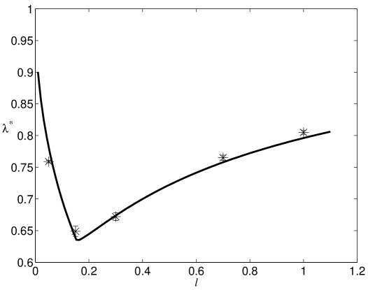
Figure 1: Variational estimate on the second eigenvalue for the one dimensional Gaussian problem using the RWMH method, with $k=1.0$. The variational estimate is the solid line and the empirically determined values are marked with stars. Some of the empirical values seem to be less than the lower bound, but this is due to inaccuracies in their estimation. The optimum occurs at $l\approx 0.165$.

The variational bound tightly matches the empirical obtained eigenvalue estimates in this case, and an optimum step size $l$ can be ascertained. Clearly our $l=1$ initial guess for the best scaling is far from optimal.

It is also worth comparing the optimal step scale with those obtained from different methods. In (Roberts and Gilks, 1997; Roberts and Rosenthal, 2001), a derivation of the optimal step size and acceptance rate is proposed based on minimizing the integrated autocorrelation time of an arbitrary function of the chain’s states in stationarity. By approximating the chain as an infinite dimensional diffusion process, formulas are derived for the optimal scaling of steps. For our one dimensional Gaussian target density, the proposal density’s optimal variance is suggested to be $(1/2.38)^{2}=0.176$ which is surprisingly close to the estimate we have obtained using the variational method from Fig. 1, $l\approx 0.165$. However, given the infinite dimensional limit in which the former approximation is made, and the different convergence criterion based on autocorrelation time rather than second eigenvalue, the agreement may be merely coincidental.

Moving to the one dimensional smart Monte Carlo, we have a Gaussian proposal density of the form :

$$q(x,y)=\sqrt{\frac{l}{2\pi}}\exp\left(-\frac{1}{2}l\left(y-(x-\frac{k}{h}x)\right)^{2}\right)$$ (8)

where $1/l$ is the variance of the random part of the step and $1/h$ is the scale of the deterministic part. (Letting $h\to\infty$ we recover the RWMH algorithm of Eqn. 7.)

Taking $h=k$ corresponds to performing a Newton step at every iterate of the algorithm. Thus, since the log of the target density is purely quadratic, the current point will always be returned to the extremum at $0$ by the deterministic component of the smart Monte Carlo step and the random component will give a combined move drawn from $q(x,y)=q(y)=\sqrt{l/(2\pi)}\exp\left(-ly^{2}/2\right)$, which has the form of an independence sampler (Robert and Casella, 1999). If we then also choose $l=k$, we see immediately that we are generating moves from the target distribution from the beginning, i.e. we have convergence in one step starting from any initial distribution.

In real problems, however, $-\log(\pi(x))$ will not be quadratic. We may obtain an estimate for $l$ and $h$ by considering its quadratic approximation or curvature but in many cases those estimates will have to be adjusted. If the curvature is very small (or in multidimensional problems if the quadratic approximations are close to singular), the parameters will have to be increased to provide a step size control to prevent wildly unconstrained moves (analogous to the application of a trust region in optimization methods (Dennis and Schnabel, 1983)). If the curvature is large but we believe that the target density is multimodal, we need to decrease the parameters to allow larger steps to escape the local extrema. Therefore we examine in the following the dependence of the convergence rate as we vary both of the parameters $l$ and $h$.

The acceptance probability Eqn. 1 has two functional forms separated by a boundary in the $(x,y)$ plane given by

$$\left(k+l\frac{k}{h}\left(-2+\frac{k}{h}\right)\right)(y^{2}-x^{2})=b(k,h,l)(y^{2}-x^{2})=0\enspace.$$ (9)

In particular, the acceptance probability is

$$\alpha(x,y)=\mbox{min}\left(\exp\left(-\frac{1}{2}b(k,h,l)(y^{2}-x^{2})\right),1\right)\enspace.$$ (10)

Now we have a complication over the RWMH method because depending on the sign of the coefficient function $b(k,h,l)$ in Eqn. 9, we find that either $\alpha(x,y)<1$ on $|y|\geq|x|$, $\alpha(x,y)=1$ on $|y|<|x|$ or vice versa. This is shown in Fig. 2.

            

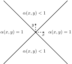
          (a)                                      (b)                                              (c)

Figure 2: Regions in xy plane where acceptance probability $\alpha(x,y)<1$ or $\alpha(x,y)=1$, when (a) $b(1,h,l)\geq 0$ and (b) $b(1,h,l)<0$. The equation for the boundary is shown in (c), see Eqn. 9 with $k=1.0$. (The RWMH algorithm will only have regions described by (a).)

As before, for a given value of $h$ and $l$, we need to break up the double integrals of the scalar product $(v_{a},\mathcal{S}v_{a})$, Eqn. 6, into the appropriate regions. Our choice of variational function is the same as before (since the target density is the same) and we again can get an explicit (but complicated) expression for Eqn. 6 which we maximize with respect to $a$. The results of this analysis are shown in Fig. 3 (a), where we fix $k=1.0$ and vary $h$, $l$. We have confirmed that these lower bounds are quite accurate as shown in Fig. 3 (b).

       

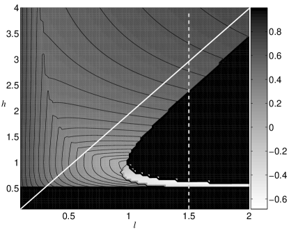
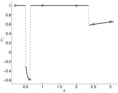
              (a)                                                                            (b)

Figure 3: Estimate of second eigenvalue for the symmetrized smart Monte Carlo operator. (a) $k=1$ is fixed and $h$, $l$ are allowed to vary. $h=1.0,l=1.0$ is the optimal scaling for deterministic and random parts of the step. The solid diagonal line is the parameter restrictions that yield the MALA algorithm (see text). (b) We take a slice through this surface at $l=1.5$ and empirically determine the second eigenvalue at points along this curve (stars). The error bars are too small to be seen. Dashed lines are discontinuities.

The remarkable feature of these results is that even for this simple Gaussian problem, the selection of step scale parameters $h$, $l$ is critical to achieve convergence. As already mentioned, there is a trivial choice of optimum with $h=l=k=1$ that gives one step convergence from any initial distribution (and therefore $\lambda^{*}=0$). However, if we change parameters infinitesimally such that $l=1+\epsilon,h=1$ ($\epsilon>0$) we go through a discontinuous transition where we see no convergence from any initial distribution. This can be understood by recognizing that after one step we will have a proposal density (before accept/reject) $\propto\exp(-(1+\epsilon)x^{2}/2)$ which has a factor $\exp(-\epsilon x^{2}/2)$ less probability in its tails than the target density. Suppose there is an initial distribution or point mass concentrated at $x=\sqrt{2M}/\sqrt{\epsilon}$, $M>>1$. The proposed step of the smart Monte Carlo algorithm, starting at $x$, will revisit $x$ too infrequently by a factor $\exp(-M)$. Thus detailed balance will force the transition $x\to 0$ to be accepted with a probability of only $\exp(-M)$, and thus the initial distribution will take an arbitrarily long time to converge to the target density.

More formally, we can compute the probability of rejection, $r(x)=1-\int t(x,y)dy$, when $h,l$ are as above and we find,

$$r(x)=\Phi\left(\sqrt{\frac{1+\epsilon}{2}}x\right)-\exp\left(\frac{1}{2}b(k,h,l)x^{2}\right)\frac{1+\epsilon}{1+\epsilon+b(k,h,l)}\Phi\left(\frac{1+b(k,h,l)+\epsilon}{2}x\right)$$

where $b(k,h,l)<0$ and $\Phi$ is the cumulative normal $(0,1)$ distribution function. We note that $\mbox{ess sup }r(x)=1$ by continuity of $r(x)$, and then we use Proposition $5.1$ from (Roberts and Tweedie, 1996a) to conclude that the Markov chain is no longer geometrically convergent for these values of $h$ and $l$.

In fact this is only one of the two disconnected regions where no convergence is observed in Fig. 3. The largest of the two (with $h>1/2$) is defined exactly by the equation $b(1,h,l)<0$ (compare Fig. 2(c) with Fig. 3 (a)). In this region the bound on the second eigenvalue approaches $1$ as the variational parameter, $a\to 0$. This corresponds to a perturbation on the target density of $x\sqrt{\pi(x)}$ for the unsymmetrized MCMC operator $\mathcal{L}$. In other words, we have a test distribution that has exponentially more probability in its tails than the target density. For initial states $x$ arbitrarily far away from the origin, the acceptance probability $\alpha(x,y)$ in the region $|y|<|x|$ is arbitrarily small. To see this, note that Eqn. 10 is an exponentially decaying function of $y^{2}-x^{2}$ in this region, and given the form of the proposal density Eqn. 8, we see that the expected value of $y^{2}-x^{2}$ is arbitrarily large and negative. Thus states far out will never be “allowed back” and the fat tails of $\sqrt{\pi(x)}$ will never shrink back down those of $\pi(x)$. Furthermore, moves $x\to y$ where $|y|\geq|x|$ are always accepted (because $\alpha(x,y)=1$ on $|y|>|x|$) which simultaneously prevents convergence. The situation is analogous to that described for $l=1+\epsilon$ and $h=k=1$, except now there is a cutoff both on the deterministic step and the random step. A typical example of this is shown in Fig. 4. Once we cross to the $b(1,h,l)\geq 0$ region, moves $x\to y$ where $|y|<|x|$ are always accepted by Eqn. 10 (Fig. 2 (a)). Therefore excess probability in the tails is allowed to flow back into the central part of the distribution and the convergence is not blocked.

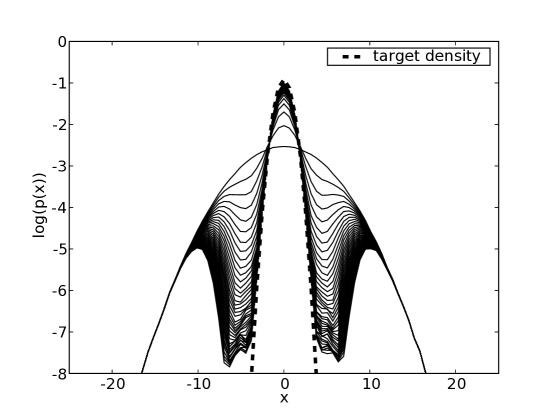
Figure 4: Forty iterates of the smart Monte Carlo algorithm (solid lines), Eqn. 8, when the initial distribution is normal with standard deviation five times the Gaussian target density (dashed line). Parameters are chosen to be in the region of no convergence ($h=2.0$, $l=1.5$), see Fig. 3 (a). We see that the tails of the initial distribution are essentially unchanging after many iterates and have failed to converge to the target density

In the second region where no convergence is observed, ($h<1/2$ in Fig. 3), we have a situation where the deterministic step alone (taking $l\to\infty$) leads to the proposed moves being generated by an unstable mapping, from the $(n-1)^{th}$ to $n^{th}$ iterate: $x^{(n)}=x^{(n-1)}-\beta x^{(n-1)}$ where $\beta>2$. The trial variational function for this situation also maximizes the bound as $a\to 0$, again implying that the tails are not decaying to the stationary distribution. The reason is that, even when $l<\infty$, we have a situation in which the expected or mean position of a state $x$ after one step is $y$ where $|y|\geq|x|$. Thus excessive probability in the tails cannot be shifted inward to match the target density.

The lack of convergence in this region was already noted for the Metropolis Adjusted Langevin Algorithm (MALA), a special case of the SMC algorithm where $h=2l$. As shown in (Roberts and Tweedie, 1996b), if $\pi$ is bounded, a sufficient condition for MALA to fail to be geometrically ergodic is

$$\liminf_{|x|\to\infty}\frac{|\nabla\log\pi(x)|}{|x|}>\frac{4}{s}$$

where $s$ is the single stepsize control parameter for that algorithm. The equivalence to the SMC method is established by setting $l=1/s$. Thus, for the Gaussian target density $\pi$, the condition is $l<1/4$. Referring to the solid white line in Fig. 3(a), the non-convergent parameter regime for MALA lies along the line segment $h=2l$ with $l<1/4$ which matches exactly with the boundary we have determined using the variational method.

The $h=1/2$ “trough” is a special case where we have oscillatory behavior. That is, the second eigenvalue is negative but greater than $-1$ and in fact convergence does occur. Interestingly setting $h=k/2$ means that $b(k,h,l)=k$ and the acceptance probability of Eqn. 10 looks again like that of the RWMH algorithm, but the convergence is actually faster. In a sense, given that the deterministic part of the step moves $x\to-x$ and the target distribution is symmetric, the oscillatory behavior allows the chain to sample the distribution twice as fast.

III.2 Quartic target density

In scientific or statistical applications where MCMC is used, the log of the target density will ordinarily have higher order terms beyond the quadratic order we studied in the previous section. For example, in a Bayesian inference problem the posterior distribution will rarely have a simple Gaussian form. Both finding the maximum a posteriori parameter estimates and sampling from the posterior are made more difficult in the presence of these higher order terms.

Therefore, we wish to extend the previous example by studying a target distribution of the form $\pi(x)=(2^{(3/4)}k^{(1/4)}/\Gamma(1/4))\exp\left(-kx^{4}/2\right)$. Here, the log of the target density is quartic and the proposal density (Gaussian) no longer has the same form as the target density. We would like to understand the performance of the Monte Carlo algorithms in this circumstance. (The test distribution is taken to be $\propto x\exp\left(-ax^{4}/2\right)$, i.e. in the orthogonal space to the stationary distribution).

The goal is to estimate the optimal value of $l$, as before. We can argue approximately that the step scale should be such that $kx^{4}/2\approx 1$ for a typical move $x$, i.e. the change in energy is about $1$ and the acceptance probability is therefore $\exp(-1)$. This gives a typical value for $x^{2}=\sqrt{2}/\sqrt{k}$. Since the proposal density is Gaussian with variance $1/l$, we therefore would naively predict $l=\sqrt{k}/\sqrt{2}$. Applying the variational method, we were unable to find a closed form solution to Eqn. 6 so we had to resort to numerical integrals in determining the bound in Eqn. 5. The results are shown in Fig. 5 for the RWMH method; it suggests an optimal choice for the step size parameter, $l$, which is an improvement over our initial guess of $1/\sqrt{2}\approx.71$ (when $k=1$). Using the formulas for the optimal step scale from (Roberts and Rosenthal, 2001) coincidentally yields about $.71$, also a little off from our variational estimate.

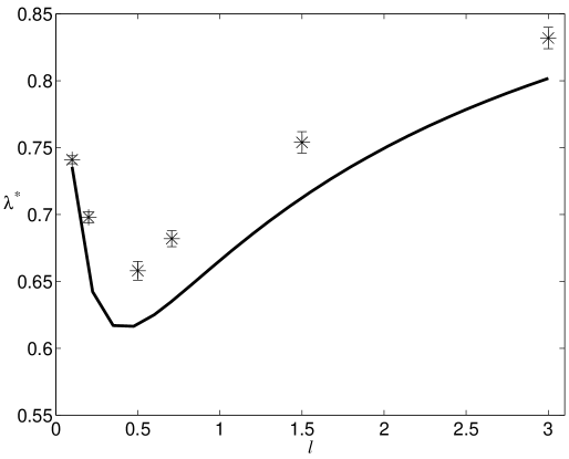
Figure 5: Second eigenvalue estimate from the variational method (solid line) and empirical estimates (stars), for the quartic target density ($k=1$) using the RWMH method, Eqn. 7. The numerical values for $\lambda^{*}$ are now estimated by taking the ratio of the discrepancy from the target density in subsequent iterates and finding a single multiplicative factor which describes the decay. This is done rather than using functional forms analogous to Hermite polynomials to fit the decay, because it appears that there may be more significant contributions from higher order terms. This also explains why the lower bound shown differs more than in Fig. 1 and Fig. 3 (b). The data point shown at $l=1/\sqrt{2}\approx.71$ (see text) does not appear to be optimal.

Turning to the smart Monte Carlo algorithm, if we wish to make the deterministic part of the proposed move a Newton step using the Hessian of $-\log(\pi(x))$ at $x=0$ we are left with a singular Hessian and an infinite deterministic step, reinforcing the need for the step length control parameter, $h$.

Surprisingly, we find that, independent of the value of $h$ and $l$, ($k$ fixed at $1$), the scalar product $(v_{a},\mathcal{S}v_{a})\to 1$ as $a\to 0$. Thus there are no choices of scaling parameters which will lead to convergence. This is borne out by numerical simulation, see Fig. 6 for the changes in an initial density under many iterates of the algorithm with an arbitrary choice for $s$, $h$.

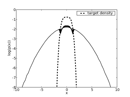
Figure 6: Forty iterates of the smart Monte Carlo algorithm (solid lines), Eqn. 8, when the target density is quartic (dashed line). The initial distribution of points is normal with standard deviation about five times that of target density (dashed line). Parameters are arbitrarily chosen as ($h=1.0$, $l=1.0$), and we see that the tails of the initial distribution are unchanged for every iterate of the algorithm. Other parameter sets tested lead to the same behavior.

The failure of the smart Monte Carlo method for the quartic problem is clearly due to non-convergence of the tails of the distribution, and can be seen by analyzing the integrals defining the operator, Eqn. 6, and noting that they all tend to zero as the variational parameter tends to zero, independent of the choice for $k$, $h$ and $l$.

As a partial check on this result, we again apply the condition derived in (Roberts and Tweedie, 1996b) for the MALA algorithm, which states that geometric convergence is not possible when $\liminf_{|x|\to\infty}|\nabla\log\pi(x)|/|x|>4/s$ where $s$ is the step scale parameter. Now, for the quartic density $\pi$, the quantity on the left of the inequality $\to\infty$, so no value of $s$ can give geometric convergence. MALA is a special case of the SMC algorithm, but we have shown here that the latter also has convergence problems indicated by $\lambda^{*}\to 1$, for all values of its scaling parameters, $h$ and $l$.

The Gaussian and quartic problems are representative examples of target densities on which we have tested the smart Monte Carlo method. As we have seen there are severe convergence problems on these distributions. We would expect that for real applications, where the log of the target density would contain components of these and higher order nonlinearities, similar convergence difficulties for the smart Monte Carlo method would occur. It may well be that in applications where the method is extensively used (e.g. (Hu et al., 2006; Kumar et al., 1996; Jardat et al., 1999)) the convergence criteria are less precise than ours. For example, it may be acceptable to merely monitor the variance of some function of the state space variables and conclude that convergence has been achieved when it ceases to change appreciably, or as in (Roberts and Rosenthal, 2001), define efficiency by the integrated autocorrelation time.

IV Multidimensional target densities

For multidimensional problems, it is quite common to find a large range of scales associated with the target density (Brown and Sethna, 2003; Gutenkunst et al., ; Waterfall et al., ). That is, the curvature of the probability density along some directions in the parameter space is much larger than in other directions. Clearly, if an MCMC method is not designed to take these different scales into account through importance sampling, the algorithm will perform very poorly. If the curvature is very high in a particular direction and we try to take a moderately sized step, it will almost certainly be rejected but if we take small steps in directions that are essentially flat the MCMC algorithm will be very slow to equilibrate. We would like to show explicitly here what happens to the convergence rate when the scale of the problem has been underestimated or overestimated.

The variational calculations for the one dimensional examples of the previous section either yielded explicit formulas or gave integrals that were relatively fast to compute numerically. However as we go to multiple dimensions neither of these features are present, in general. Typically the integrals describing $(v_{a},\mathcal{S}v_{a})$ will not factor into one dimensional integrals. For Gaussian target densities the full space is broken into regions analogous to those in Fig. 2, described by an equation like $y^{t}Ay\geq x^{t}Ax$ where $A$ is a symmetric $n$ by $n$ matrix which is not necessarily positive definite. For the RWMH algorithm applied to a multivariate Gaussian target density with inverse covariance matrix $K$, we have $A=K$, and therefore all the dimensions are coupled through the energy change, $\Delta E=y^{t}Ky-x^{t}Kx$. We would still like to be able to get a lower bound on $\lambda^{*}$, and to this end note that any test function orthogonal to the target density will work in Eqn. 5; the bound does not explicitly require a variational parameter, however without it the estimate will be less accurate. It is still necessary to make choices for the test functions that are both tractable in computing $(v,\mathcal{S}v)$ and are “difficult” functions for the given algorithm to converge from, i.e. have a significant component along the true second eigenfunction.

As an example, take the multivariate Gaussian distribution of the form

$$\pi(x)=\frac{\sqrt{|K|}}{(2\pi)^{\frac{n}{2}}}\exp\left(-\frac{1}{2}x^{t}Kx\right)$$ (11)

with $x=(x_{1},...,x_{n})$, and consider using the MH algorithm with importance sampling, i.e.

$$q(x,y)=\frac{\sqrt{|L|}}{(2\pi)^{\frac{n}{2}}}\exp\left(-\frac{1}{2}(y-x)^{t}L(y-x)\right)$$

where again $L$ is the inverse covariance matrix/step size control term and to simplify we assume that both $K$ and $L$ are diagonal. Without any analysis we might guess that the optimum choice for $L$ is $K$.

First we construct a test function that will provide a useful bound when the proposed steps are too large for the natural scale of the problem. For simplicity, consider putting a delta function distribution at the origin. If we take large steps the acceptance probability should be low and there will be a large overlap between the initial state and the final state. In the limit that the proposed steps have infinite length, the initial state will not be changed at all and the bound on the second eigenvalue in absolute value will approach one. To do this more carefully we define a test function which is a Gaussian whose variance will ultimately be taken to zero to represent the delta function. However, we also need to add another term to ensure the test function is orthogonal to the target density, in order to apply the variational bound. Therefore, for the unsymmetric operator we write the test function as : $u_{\sigma}(x)=-A\pi(x)+Bw_{\sigma}(x)$ where $w_{\sigma}(x)$ is the probability density for a multivariate Gaussian with covariance matrix $\sigma^{2}I$ and $A$ and $B$ are constants. For the symmetrized operator the trial function is transformed to $v_{\sigma}(x)=-A\sqrt{\pi(x)}+Bw_{\sigma}(x)/\sqrt{\pi(x)}$. $A$ and $B$ are constrained to satisfy the orthogonality relation $(v_{\sigma},\pi)=0$ and a normalization $(v_{\sigma},v_{\sigma})=1$. These lead to the conditions

$$A=B\quad\mbox{ and }\quad B^{2}\int\left(\frac{w_{\sigma}(x)}{\sqrt{\pi(x)}}\right)^{2}\,dx=1+B^{2}\enspace.$$

Then it can be seen that

$$(v_{\sigma},\mathcal{S}v_{\sigma})=-B^{2}+B^{2}\left(\mathcal{S}\frac{w_{\sigma}(x)}{\sqrt{\pi(x)}},\frac{w_{\sigma}(x)}{\sqrt{\pi(x)}}\right)$$

where we have used the orthogonality condition, the fact that $w_{\sigma}(x)$ integrates to $1$ and that $\mathcal{S}$ is self-adjoint. Writing out the operator $\mathcal{S}$ explicitly we get

$$\left(\mathcal{S}\frac{w_{\sigma}(x)}{\sqrt{\pi(x)}},\frac{w_{\sigma}(x)}{\sqrt{\pi(x)}}\right) = \int\int\frac{w_{\sigma}(x)}{\sqrt{\pi(x)}}s(x,y)\frac{w_{\sigma}(y)}{\sqrt{\pi(y)}}\,dxdy-\int\int t(x,y)\left(\frac{w_{\sigma}(x)}{\sqrt{\pi(x)}}\right)^{2}\,dxdy$$

$$+\int\left(\frac{w_{\sigma}(x)}{\sqrt{\pi(x)}}\right)^{2}\,dx\enspace.$$

The last term on the right hand side is $(1+B^{2})/B^{2}$, making use of the normalization condition, so we are left with

$$(v_{\sigma},\mathcal{S}v_{\sigma})=B^{2}\int\int\frac{w_{\sigma}(x)}{\sqrt{\pi(x)}}s(x,y)\frac{w_{\sigma}(y)}{\sqrt{\pi(y)}}\,dxdy-B^{2}\int\int t(x,y)\left(\frac{w_{\sigma}(x)}{\sqrt{\pi(x)}}\right)^{2}\,dxdy+1\enspace.$$

Since we are ultimately taking a limit as $\sigma\to 0$ ($w_{\sigma}\to$ a delta function) we can make approximations to these integrals as follows :

$$\int\int\frac{w_{\sigma}(x)}{\sqrt{\pi(x)}}s(x,y)\frac{w_{\sigma}(y)}{\sqrt{\pi(y)}}\,dxdy\approx s(0,0)\int\int\frac{w_{\sigma}(x)}{\sqrt{\pi(x)}}\frac{w_{\sigma}(y)}{\sqrt{\pi(y)}}\,dxdy$$

and

$$\int\int t(x,y)\left(\frac{w_{\sigma}(x)}{\sqrt{\pi(x)}}\right)^{2}\,dxdy\approx\int t(0,y)\,dy\int\left(\frac{w_{\sigma}(x)}{\sqrt{\pi(x)}}\right)^{2}\,dx\enspace.$$

Finally by taking $\sigma\to 0$ we have the expression

$$(\mathcal{S}v_{0},v_{0})=1-\int t(0,y)\,dy\enspace.$$

As already mentioned, for the multidimensional problem we expect different functional forms for the kernels $s(x,y)$ and $t(x,y)$ depending on the initial and final state $(x,y)$ and this is what makes decoupling the integrals difficult. However for this choice of test function the equation for the boundary (with $x=0$) is given by $y^{t}Ky=0$ and since $K$ is positive semidefinite we always stay on one side of the boundary (the energy never decreases from the initial distribution placed at $x=0$). Then

$$(\mathcal{S}v_{0},v_{0}) = 1-\frac{\sqrt{|L|}}{(2\pi)^{\frac{n}{2}}}\int\exp\left(-\frac{1}{2}y^{t}(K+L)y\right)\,dy$$ (12)

$$= 1-\prod_{i=1}^{n}\sqrt{\frac{l_{i}}{l_{i}+k_{i}}}\enspace.$$ (13)

where $l_{i}$ and $k_{i}$ are the diagonal elements of the diagonal matrices $L$ and $K$, respectively. With no importance sampling we would have $L=kI$ where $k$ would be chosen to make sufficiently large steps to enable it to sample $\pi(x)$. A rough argument as follows can give some insight into the form of Eqn. 13 : $1/\sqrt{l_{i}}$ is a measure of the scale in the $i^{th}$ coordinate direction of the proposal density, $1/\sqrt{k_{i}}$ is the scale in the $i^{th}$ coordinate direction of the target density. Suppose that $l_{i}\ll k_{i}$ for each $i$, that is the scales of the proposal density are too large in all directions. Then the ratio of the mean volume of moves generated by $q(0,y)$ to the volume occupied by $\pi(y)$ is exactly $\prod_{i=1}^{n}\sqrt{l_{i}}/\sqrt{k_{i}}$. Intuitively, this ratio is proportional to the acceptance probability, and in the regime $l_{i}\ll k_{i}$ the acceptance probability determines the convergence properties.

We want to use Eqn. 13 to show how choosing step sizes too large even in one direction will result in a very inefficient algorithm. Suppose that for all but one of the directions we make $l_{i}=k_{i}$, $i=1,\ldots,n-1$ which would be roughly the correct scaling in those directions. Then the bound on the second eigenvalue is

$$(\mathcal{S}v_{0},v_{0})=1-\sqrt{\left(\frac{1}{2}\right)^{n-1}}\sqrt{\frac{1}{1+k_{n}/l_{n}}}\enspace.$$ (14)

From this we can see that as we go to larger and larger step sizes relative to the scale in the last direction ($k_{n}/l_{n}\to\infty$), the bound on $\lambda^{*}$ increases to $1$. Conversely we can argue that if one of the directions of the target density has a scale that is considerably smaller than the step scales being used in the proposal density, we will get very few acceptances and the convergence rate will be close to $0$. Hence we see explicitly the need for importance sampling to accelerate convergence.

We would also like to address what happens in the other limit as the step size becomes excessively small compared to the natural scale of the problem. (In fact Eqn. 13 gives a lower bound of zero in that case which is not surprising as it is based essentially on the term in the operator equation which gives the probability of staying at the current state. If we take infinitesimally small steps, the acceptance probability will be one and we will never stay at the current state). When the step scales are infinitesimally small we expect intuitively that the bound on the second eigenvalue will also approach one; even though the acceptance ratio is close to one, very small steps will never be able to “explore” the target distribution sufficiently. To compute this limit, we propose a test function which has components of the target density in all directions except the last, where it has an antisymmetric form to make sure it is orthogonal to the target density. With respect to the symmetrized operator $\mathcal{S}$ this means

$$v(x)\propto x_{n}\prod_{i=1}^{n}\sqrt{\pi_{i}(x_{i})}\enspace.$$ (15)

Here $\sqrt{\pi_{i}(x_{i})}$ is the one dimensional Gaussian density which is the $i^{th}$ factor in a diagonalized multivariate Gaussian density. (Recall that since $\pi(x)$ is an eigenfunction of $\mathcal{L}$, then $\sqrt{\pi(x)}$ is an eigenfunction of $\mathcal{S}$.) We still have the problem of decoupling the $n$-dimensional multivariate problem into $n$ one dimensional problems. To manage this we use a device to re-express the operator equation , Eqn. 6, explicitly in terms of the change $\frac{1}{2}(y^{t}Ky-x^{t}Kx)$. (i.e. $-\log{\frac{\pi(y)}{\pi(x)}}$), which we denote by $\Delta E$. That is

$$(v,\mathcal{S}v) \,=\int\int v(x)s(x,y)v(y)\,dxdy-\int\int t(x,y)\left(v(x)\right)^{2}\,dxdy+1$$

$$= \int\int x_{n}\pi(x)q(x,y)\left(\int\mbox{min}(e^{-\Delta E},1)\,\delta\left(\Delta E-\frac{1}{2}\sum_{i=1}^{n}k_{i}(y_{i}^{2}-x_{i}^{2})\right)\,d\Delta E\right)\,dxdy-$$

$$\int\int x_{n}^{2}\pi(x)q(x,y)\left(\int\mbox{min}(e^{-\Delta E},1)\,\delta\left(\Delta E-\frac{1}{2}\sum_{i=1}^{n}k_{i}(y_{i}^{2}-x_{i}^{2})\right)\,d\Delta E\right)\,dxdy$$

Then we use the integral representation of the delta function $\delta(x)=\frac{1}{2\pi}\int\exp(-{\rm i}wx)\,dw$, factor $q(x,y)=\prod_{i=1}^{n}q_{i}(x_{i},y_{i})$, and rearrange the order of integration to give :

$$(v,\mathcal{S}v)=\frac{1}{2\pi}\int\mbox{min}(\exp(-\Delta E),1)\left(\int A(w)\exp(-{\rm i}w\Delta E)\,dw\right)\,d\Delta E$$ (16)

where $A(w)$ contains the integration over the now decoupled $(x,y)$ coordinates :

$$A(w) = \left(\prod_{i=1}^{n-1}\int\int\pi_{i}(x_{i})q_{i}(x_{i},y_{i})\exp\left(\frac{1}{2}{\rm i}wk_{i}(y_{i}^{2}-x_{i}^{2})\right)\,dx_{i}\,dy_{i}\right)\times$$ (18)

$$\int\int(x_{n}y_{n}-x_{n}^{2})\pi_{n}(x_{n})q_{n}(x_{n},y_{n})\exp\left(\frac{1}{2}{\rm i}wk_{i}(y_{n}^{2}-x_{n}^{2})\right)\,dx_{n}\,dy_{n}$$

$$= \prod_{i=1}^{n-1}\frac{1}{(1+\frac{k_{i}}{l_{i}}w(-{\rm i}+w))^{\frac{1}{2}}}\,\frac{{\rm i}\frac{k_{n}}{l_{n}}w}{(1+\frac{k_{n}}{l_{n}}w(-{\rm i}+w))^{\frac{3}{2}}}$$ (19)

Note that the complex integral with respect to $dw$ has a branch point at the roots of $(1+\frac{k_{n}}{l_{n}}w(-{\rm i}+w))^{\frac{3}{2}}$ which lie on the imaginary axis at $r_{1}$ and $r_{2}$. It simplifies the analysis to consider the situation $k_{i}=l_{i}$ for $i=1,\ldots,(n-1)$ and assume that $n-1$ is even. This way, the roots of $(1+w(-{\rm i}+w))^{\frac{n-1}{2}}$, $r_{1,0}$ and $r_{2,0}$, are $(n-1)/2$ order poles and not branch points, also on the imaginary axis. If we now also assume that $k_{n}<s_{n}$, then we can take a contour as shown in Fig. 7 when $\Delta E<0$ and a similar one in the lower imaginary plane when $\Delta E>0$.

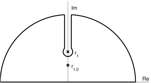
Figure 7: Contour used to evaluate Eqn. 19 when $\Delta E<0$. $r_{1}$ is a branch point and $r_{1,0}$ is a pole of order $(n-1)/2$. The contour is the same for $\Delta E<0$ except restricted to the negative imaginary plane.

Thus Eqn. 19 is reduced to a residue term and a real integral which needs to be evaluated numerically. The result is plotted for $n=11$ in Fig. 8 along with the bound that came from Eqn. 14. Thus we see the trade off between taking large steps that potentially can explore the space quickly but have a higher chance of being rejected and taking small steps which will have a high acceptance probability but will be unable to sample the space quickly.

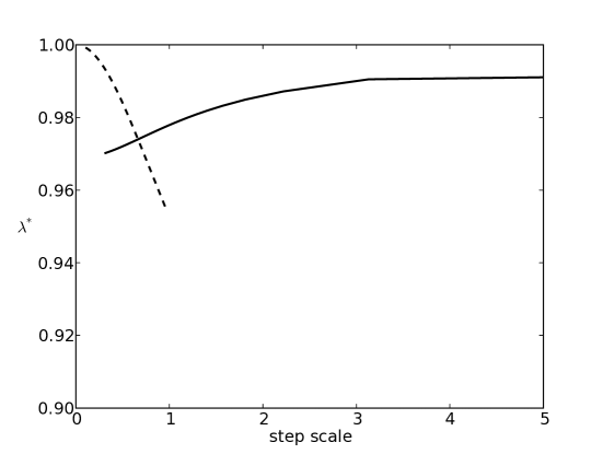
Figure 8: Lower bound on second eigenvalue for the multivariate Gaussian problem, Eqn. 11, with $n=11$. Step scale = $\sqrt{1/l_{n}}$. $k_{n}=1$ sets the scale of the target density in the last direction. The test function is chosen as the negative of the target density perturbed by a delta function (solid line) or as the target density itself in all directions but the last (dashed line). The estimate for the lower bound is a maximum of the two curves.

As we saw when doing the full variational calculation for the one dimensional problems, the best step scale to use is not what we may have guessed; the natural choice $l_{n}=k_{n}=1$ here does not appear to minimize the second eigenvalue. We believe this kind of “approximate” variational approach may be a useful way to deal with problems which are difficult to analyze otherwise.

V Conclusion

By applying a variational method, it is possible to obtain an accurate (lower bound) estimate for the second eigenvalue of an MCMC operator and thus bound the asymptotic convergence rate of the chain to the target distribution. Given such an estimate we can optimally tune the parameters in the proposal distribution to improve the performance of the algorithm. The procedure has a role to play between the various numerical algorithms that perform convergence diagnostics before the full simulations are run, to allow the user to manually tune parameters, and the adaptive schemes (Gilks et al., 1998; Atchade, 2005) that require no preliminary exploration. The simulations we performed to confirm our variational bounds in the case of a one dimensional target density and varying one step scale parameter, Fig. 1 and Fig. 3 (b), would be infeasible to do as we move to higher dimensions and as we vary additional algorithm parameters. It is in those situations that the variational method can more efficiently identify regions of optimality.

In addition, the variational method allows us to discover weaknesses in variants of the Random Walk Metropolis-Hastings algorithm which on the surface appear to be reasonable prescriptions for sampling the target density. This is most dramatically seen in the smart Monte Carlo method discussed above which apparently has serious flaws for even the simplest of one dimensional target densities. Although the smart MC method has been widely used in molecular dynamics applications (Hu et al., 2006; Kumar et al., 1996; Jardat et al., 1999) the scales are often chosen by physical considerations (for example, to not exceed significantly the step sizes needed to accurately describe the dynamical evolution of the system) and furthermore, the diagnostics of convergence are not as rigorous as ours; typically a physical quantity is monitored till it appears to reach an equilibrium value, the rare events which correspond to the tails of the target distribution are possibly of lesser importance in those studies. Therefore the convergence problems we have discussed here specifically in relation to the smart Monte Carlo method, to our knowledge, have not been previously examined. Presumably the convergence problems can be corrected by a more careful discretization of the underlying diffusion equations, as was shown for the related Langevin-type methods (Stramer and Tweedie, 1999).

It would be interesting to apply the same technique to the more broadly used gradient based hybrid MC algorithms (Duane et al., 1987) and other non-adaptive accelerated methods (e.g. parallel tempering (Earl and Deem, 2005)) where the alternative techniques for determining convergence via diffusion approximations may be harder to apply. More generally, the variational analysis could be a useful tool in making comparisons between the convergence properties of the latest MCMC algorithms without extensive numerical simulation.