Also at ]Department of Earth System Science and Technology, Kyushu University

Kinetically modified parametric instabilities of circularly-polarized Alfvén waves:
Ion kinetic effects

Abstract

Parametric instabilities of parallel propagating, circularly polarized finite amplitude Alfvén waves in a uniform background plasma is studied, within a framework of one-dimensional Vlasov description for ions and massless electron fluid, so that kinetic perturbations in the longitudinal direction (ion Landau damping) are included. The present formulation also includes the Hall effect. The obtained results agree well with relevant analysis in the past, suggesting that kinetic effects in the longitudinal direction play essential roles in the parametric instabilities of Alfvén waves when the kinetic effects react “passively”. Furthermore, existence of the kinetic parametric instabilities is confirmed for the regime with small wave number daughter waves. Growth rates of these instabilities are sensitive to ion temperature. The formulation and results demonstrated here can be applied to Alfvén waves observed in the solar wind and in the earth’s foreshock region. (accepted to Physics of Plasmas)

Circularly polarized, finite amplitude Alfvén waves are ubiquitous in collisionless space plasmas, for example in the solar wind, and also in the foreshock region of planetary bowshocks where ions backstreaming from the bowshockeastwood05 generate large amplitude Alfvén wavesagim95 ; wang03 . Parametric instabilities are of particular interest for dissipation of quasi-parallel Alfvén waves there, since they are typically robust for linear ion-cyclotron damping (due to small wave frequencies) and for linear Landau damping (due to small propagation angle relative to the background magnetic field).

Within a framework of the Hall-magnetohydrodynamic (MHD) equations, a number of research has been carried out on the parametric instabilities of parallel propagating, circularly polarized finite amplitude Alfvén waveshollweg94 ; wong86 ; longtin86 ; terasawa86 , which is an exact solution of the nonlinear Hall-MHD equation sets. Among various parametric instabilities, modulational, decay, and the beat instabilities are important. In general, growth rates of the instabilities depend on the parent wave amplitude, wave number, polarization, and the ratio of the sound to the Alfvén velocity ($=C_{s}/C_{A}=\sqrt{\beta_{f}}$).

While a large number of past studies deal with the instabilities within the framework of fluid theory, since the ion beta (the ion fluid to magnetic pressure ratio) is not small in the solar wind and in the earth’s foreshock region, the ion kinetic effects cannot be neglected. From this perspective, numerical analysis using the hybrid simulation code (super-particle ions + massless electron fluid) was performed by Terasawa et. al.terasawa86 and Vasquezvasquez95 . Mjolhus and Wyllermjolhus86 ; mjolhus88 derived and discussed in detail a nonlinear evolution equation (kinetically modified derivative nonlinear Schrodinger equation, first derived by Rogisterrogister71 ), which describes the wave modulation of weakly despersive, nonlinear Alfvén waves including the ion Landau damping. Fla et. al.fla89 and Spanglerspangler89 ; spangler90 discussed the modulational instability of parallel propagating, circularly polarized Alfvén waves, and pointed out that, while the kinetic effects suppressed the parametric instabilities present in the fluid model (“conservative modulational instability (CMI)”), the ion kinetics could evoke a new instability (“resonant particle modulational instability (RPMI)”)fla89 . Inhesterinhester90 first showed the kinetic formulation for parametric decay instabilities without dispersion. Gomberoffgomberoff00 and Aranedaaraneda98 discussed the ion kinetic effects on parametric instabilities phenomenologically. Common view among past analytical works on parametric instabilities is that the ion kinetic effects expand the unstable parameter regime and reduce the maximum growth rate. Recently, Passot and Sulempassot04 derived the dispersive Landau fluid model, and made comparison with some of the other models in the past from both analytical and numerical standpointspassot04 ; bugnon04 .

Linear analysis play important role in verifying the instabilities seen in the numerical simulationvasquez95 and provide a more complete reporting of growth rates as a function of the parameters. To our knowledge, linear kinetic analysis with dispersion has not yet been demonstrated. Our aim in this study is to derive a kinetic formulation including dispersion systematically, and present a linear analysis and compare it with other analytical results. Our treatment of the ion kinetic effects is similar to that in Munoz et. al.munoz05 , in which relativistic dispersion relation for parametric instabilities in an electron-positron plasma is derived.

We consider the parametric instabilities of parallel propagating, circularly polarized finite amplitude Alfvén waves, which are the exact solution within the Hall-MHD equation sets. Assuming weak ion cyclotron damping, we include the kinetic effects only along the longitudinal $(x)$ direction. Let $f(x,t,{{\bf v}})$ be the ion distribution function, and define the integrated longitudinal distribution function,

$$g(x,t,v_{x})=\int f(x,t,{{\bf v}})dv_{y}dv_{z}.$$ (1)

Then the governing set of equations can be written as,

$${\frac{\partial{\tilde{u}}}{\partial t}} = -u_{x}{\frac{\partial{\tilde{u}}}{\partial x}}+{\frac{1}{\rho}}{\frac{\partial{\tilde{b}}}{\partial x}},$$ (2)

$${\frac{\partial{\tilde{b}}}{\partial t}} = -{\frac{\partial{}}{\partial x}}\left(u_{x}{\tilde{b}}-{\tilde{u}}+\frac{i}{\rho}{\frac{\partial{\tilde{b}}}{\partial x}}\right),$$ (3)

$${\frac{\partial{g}}{\partial t}} = -v_{x}{\frac{\partial{g}}{\partial x}}-(e_{x}+u_{y}b_{z}-u_{z}b_{y}){\frac{\partial{g}}{\partial v_{x}}},$$ (4)

$$e_{x} = -u_{y}b_{z}+u_{z}b_{y}-\frac{1}{\rho}{\frac{\partial{}}{\partial x}}\left(\frac{|b|^{2}}{2}+p_{e}\right),$$ (5)

where $\rho$ is the plasma density (quasi-neutrality assumed), ${{\bf u}}=(u_{x},u_{y},u_{z})$ is the ion bulk velocity vector, ${\tilde{b}}=b_{y}+ib_{z}$ and ${\tilde{u}}=u_{y}+iu_{z}$ are the complex transverse magnetic field and bulk velocity, respectively, and $e_{x}$ is the longitudinal electric field. All the normalizations have been made using the background constant magnetic field, density, Alfvén velocity, and the ion gyro-frequency defined at a certain reference point.

The total pressure is given as $p=p_{e}+p_{i}$, where isothermal electrons are assumed, i.e., $p_{e}=T_{e}\rho$. Also it is assumed that the ion and electron pressures are isotropic both at the zeroth and at the perturbation orders. Usual beta ratio slightly differs from the ratio between the sound and the Alfvén wave speed squared, $\beta_{f}=(\gamma_{e}\beta_{e}+\gamma_{i}\beta_{i})/2$, where $\gamma_{e}=1$ and $\gamma_{i}$ are the ratios of specific heats for electrons and ions, respectively.

At the zeroth order we consider the parallel propagating Alfvén wave given as

$${\tilde{b}}_{p} = b_{0}\exp(i(\omega_{0}t-k_{0}x)),$$ (6)

$${\tilde{u}}_{p} = u_{0}\exp(i(\omega_{0}t-k_{0}x)),$$ (7)

with $u_{0}=-b_{0}/v_{\phi 0}$, phase velocity $v_{\phi 0}=\omega_{0}/k_{0}$, $\rho_{0}=1$, $u_{x0}=0$, together with the zeroth order dispersion relation

$$\omega_{0}^{2}=k_{0}^{2}(1+\omega_{0}).$$ (8)

We adopt the notation that the positive (negative) $\omega_{0}$ corresponds to the right- (left-) hand polarized waves. For the zeroth order longitudinal distribution function, we assume $g_{0}(v_{x})=\exp(-v^{2}_{x}/v^{2}_{th})/{\sqrt{\pi}v_{th}}$ ($v^{2}_{th}=\beta_{i}$).

Then we add small fluctuations given by

$$\delta E = E_{+}\exp(i\phi_{+})+E_{-}\exp(i\phi_{-}),$$ (9)

$$\delta F = \frac{1}{2}(F_{1}\exp(i\Phi)+c.c.),$$ (10)

where $E$ represents the transverse variables (${\tilde{b}}$ and ${\tilde{u}}$), and $F$ represents the longitudinal variables ($g$, $\rho$, and $u_{x}$), $\phi_{\pm}=\omega_{\pm}t-k_{\pm}x$, $\Phi=\Omega t-Kx$, $k_{\pm}=k_{0}\pm K$, $\omega_{\pm}=\omega_{0}\pm\Omega$, and $c.c.$ denotes the complex conjugate.

Then, (2)-(5) at the first order produce

$$(\omega_{\pm}^{2}-k^{2}_{\pm}-\omega_{\pm}k^{2}_{\pm})b_{\pm}^{(*)} = \frac{k_{\pm}}{2}(b_{0}\omega_{\pm}-u_{0}k_{0})u_{x1}$$ (11)

$$-\frac{b_{0}k_{0}k_{\pm}}{2}(\omega_{\pm}+1)\rho_{1},$$

$$g_{1}(v_{x})=-\frac{K[b_{0}(b_{+}+b^{*}_{-})+T_{e}\rho_{1}]}{\Omega-v_{x}K}{\frac{\partial{g_{0}(v_{x})}}{\partial v_{x}}},$$ (12)

where $T_{e}=\beta_{e}/2$ and the asterisk denotes the complex conjugate.

Integration of the above yields

$$\rho_{1} = -K[b_{0}(b_{+}+b^{*}_{-})+T_{e}\rho_{1}]D,$$

$$D = \int_{-\infty}^{\infty}{\frac{\partial{g_{0}}}{\partial v_{x}}}\frac{dv_{x}}{\Omega-v_{x}K}=\frac{2}{v^{2}_{th}K}(1+\xi Z(\xi)),$$ (13)

where $\xi=\Omega/v_{th}/K$, and $Z(\xi)$ is the plasma dispersion function. This equation can be written as

$$\rho_{1}=A(b_{+}+b^{*}_{-}),~{}~{}A=-\frac{Kb_{0}D}{1+KT_{e}D}.$$ (14)

In a similar way, we have

$$u_{x1}=B(b_{+}+b^{*}_{-}),~{}~{}B=-K(b_{0}+T_{e}A)C,$$ (15)

$$C=\int_{-\infty}^{\infty}{\frac{\partial{g_{0}}}{\partial v_{x}}}\frac{v_{x}dv_{x}}{\Omega-v_{x}K}=v_{th}\xi D,$$ (16)

where $n_{0}=1$. Combing (11)-(16), we obtain

$$L_{+}L_{-}=L_{+}P_{-}+L_{-}P_{+}$$ (17)

where

$$L_{\pm} = \omega^{2}_{\pm}-k_{\pm}^{2}(1+\omega_{\pm}),$$ (18)

$$S_{\pm} = \frac{b_{0}k_{\pm}}{2}B-\frac{b_{0}k_{0}k_{\pm}}{2}A,$$ (19)

$$T_{\pm} = \frac{v_{0}k_{0}k_{\pm}}{2}B+\frac{b_{0}k_{0}k_{\pm}}{2}A,$$ (20)

$$P_{\pm} = S_{\pm}L_{\pm}-T_{\pm}.$$ (21)

By taking the cold limit ($\beta_{i}\sim 0$, i.e., $\xi>>1$), the dispersion relation of the Alfvén wave parametric instabilities in the Hall-MHD is obtainedterasawa86 . We note that (17) is an odd function with respect to both $\Omega$ and $K$.

Now we examine the numerical solutions of (17). First, we refer to the results by Inhesterinhester90 , in which the kinetic dispersion relation of parametric decay instability is derived without dispersion, using drift kinetic model. In order to make comparison with their results, we omit the dispersion terms in (17): the third term in the RHS of (18) and the second term in the RHS of (19). Note that in the dispersionless system, the modulational instability (both CMI and RPMI) does not occur and the growth rate of the decay instability differ from one in the dispersive systemterasawa86 . By further assuming the cold limit, our equation leads to the MHD dispersion relation obtained by Goldsteingoldstein78 and Derbyderby78 , (but not to the model by Inhester (1990)). On the other hand, numerically obtained dispersion relations based on our model and that of Inhester at least qualitatively agrees, in the sense that the ion kinetic effects enlarges the unstable parameter regime and also the maximum growth rates are reduced (Figure 1). These results are also in qualitative agreement with some of the past worksinhester90 ; bugnon04 .

Figure 1: Growth rates of the density modes (whose frequency/wave number is normalized to the parent wave parameters), driven by the decay instability of dispersionless Alfvén waves with amplitude $b_{0}=0.447$, $\beta=0.6$, and $T_{r}(=T_{i}/T_{e})=$ (a) $0$ (=fluid model, black cross), (b) $0.03$ (blue broken line), (c) $0.2$ (light blue), (d) $1$ (green dotted line), (e) $5$ (orange), (f) $\infty(T_{e}=0)$ (red solid line). The results shown here are in agreement with Inhester (1990) and Bugnon et. al.(2004).

We now turn our attention to the parametric instabilities of the dispersive Alfvén waves. Figure 2 shows the growth rates computed from (17) for right-hand polarized Alfvén waves, for various temperature ratios, $T_{r}(=T_{i}/T_{e})$. The decay-like instabilities have positive growth rates when $K>|k_{0}|=0.408$. The results here qualitatively agrees with numerical results obtained by Vasquezvasquez95 and Bugnonbugnon04 (Table 1 in both papers), which suggests that the ion kinetic effects in the longitudinal direction play essential roles in kinetic modification of the Alfvén parametric instabilities, when $\beta_{i}$ is relatively small, i.e., the kinetic effects “passively” react to the fluid dynamics.

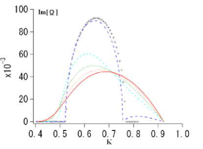
Figure 2: Growth rates of the density modes (frequency/wave number is normalized to the ion-gyrofrequency/ion inertial length), driven by the decay instability of dispersive Alfvén waves with $b_{0}=0.5$, $k_{0}=0.408$, $\omega_{0}=0.5$ (R-mode), $\beta=0.45$, and $T_{r}(=T_{i}/T_{e})=$ (a) $0$ (=fluid model, black cross), (b) $0.0227$ (blue broken line), (c) $0.36$ (light blue), (d) $1$ (green dotted line), (e) $2.75$ (orange), (f) $\infty(T_{e}=0)$(red solid line). The results agree well with Vasquez (1995) and Bugnon (2004).

Figure 3 shows the growth rates under the same parameters as in Figure 2 except that $k_{0}=0.102$ and $\omega_{0}=0.107$ (R-mode). Both regimes $K>|k_{0}|$ and $K<|k_{0}|$ are plotted. The former corresponds to the “conservative decay instability (CDI)”, which has the finite growth rate at $T_{r}=0$ as we see in Figures 1 and 2. On the other hand, the latter, the RPMI, is destabilized only for finite $T_{r}$, although the growth rate is typically 1 or 2 orders less than the CMI. The RPMI is quenched when $T_{r}=0$, suggesting that the instability is a product of Landau resonant effects (Fla et. al.fla89 , Spanglerspangler89 ; spangler90 ). The RPMI exists even at small wavenumbers.

Figure 3: Same as Figure 2 except that $b_{0}=0.5$, $k_{0}=0.102$, $\omega_{0}=0.107$ (R-mode), $\beta=0.45$, with $T_{r}(=T_{i}/T_{e})=$ (a) $0$ (=fluid model, black cross), (b) $0.0227$ (blue broken line), (c) $1(\beta_{e}=\beta_{i}=0.225)$ (green dotted line), (d) $\infty(T_{e}=0)$ (red solid line), and when $\beta_{e}=0.225$ with (e) $\beta_{i}=0.5$ (square), (f) $\beta_{i}=1.0$ (circle), (g)$\beta_{i}=2.0$ (diamond), respectively.

As shown in Figure 3 (c)-(g), the growth rate of the RPMI is sensitive to $\beta_{i}$. In particular, as $\beta_{i}$ is increased, the growth rate of the RPMI is enhanced while that of the CDI is reduced. When $\beta_{i}=2$ and $\beta_{e}=0.225$, the growth rates of both instabilities become comparable. The CDI growth rate is increased as $\beta_{f}$ (=$\beta_{e}/2$ for the present case) is reduced. The decrease of the growth rates of the CD(M)I is relaxed at large $T_{r}$ (c.f., Fig.1, 2 (e), (f)).

Finally, we discuss briefly the instability of left-hand polarized Alfvén waves (Figure 4). Under the parameters used, the CMI (the maximum growth rate $\sim 0.4$), the CDI (likewise, $\sim 0.6$), and the beat instability (likewise, $\sim 0.8$) are driven unstable at $T_{r}=0$. Figure 4 shows that the growth rate of the decay-like instability ($\sim 0.8$) exceeds that of the modulational-like instability at $T_{r}>\sim 0.2$.

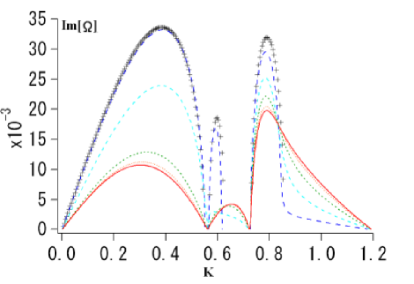
Figure 4: Same as Figure 2 except that $b_{0}=0.4$, $k_{0}=0.56$, $\omega_{0}=-0.425$ (L-mode), $\beta=0.6$, and $T_{r}(=T_{i}/T_{e})=$ (a) $0$ (=fluid model, black cross), (b) $0.03$ (blue broken line), (c) $0.2$ (light blue), (d) $1$ (green dotted line), (e) $5$ (orange), and (f) $\infty(T_{e}=0)$ (red solid line).

In the present paper we discussed the kinetically modified parametric instabilities of circularly polarized, parallel-propagating Alfvén waves within a framework of one-dimensional system, which includes longitudinal kinetic perturbations. The obtained dispersion relation (17) is numerically evaluated, and compared with relevant works in the literature. The real part of $\Omega$ in (17) is not shown here, but we have confirmed that the propagation direction of the sideband Alfvén waves and the density fluctuations are consistent with the past studies.

While our analysis includes $\beta_{i}$ as a free parameter, it should be retained at a modest value, since at high $\beta_{i}$, kinetic response of the transverse distribution function cannot be neglected, and the kinetic effects must be included in the parent wave dispersion relation (9)vasquez95 ; bugnon04 ; abraham77 ; yajima66 . Comparison of Fig.2 with past studies suggests that our assumption on basic equations is valid when $\beta_{i}=0.45$, but is not for $\beta_{i}\sim>1.5$vasquez95 . This remark also applies to simulation studies using the hybrid code: it is important to use kinetic instead of fluid dispersion relation to give initial wave when the ion beta is large.

Finally we point out that, despite the importance of the parametric instabilities in the solar wind or in the earth’s foreshock, their presence has not yet been clearly demonstrated by spacecraft experiments. Linear theory predicts that parallel propagating waves are mainly excited in the solar wind or in the earth’s foreshockgary81 ; hada87 . However, recent multi-point measurement observations suggest that these waves tend to propagate obliquely to the background magnetic fieldeastwood05 ; narita03 ; eastwood05b . Numerical simulation study using hybrid codewang03 should be effective in understanding the parametric instabilities of obliquely propagating large amplitude MHD waves. We hope the situation to change via knowledge of kinetic modification of the instabilities as well as state-of-the-art data acquisition and analysis techniques.

We thank Drs. S. Matsukiyo, V. Munoz, and T. Passot for fruitful discussions and comments. This paper has been supported by JSPS Research Fellowships for Young Scientists in Japan.

References

- (1) J. P. Eastwood, , E. A. Lucek, C. Mazelle, K. Meziane, Y. Narita, J. Pickett, and R. A. Treumann, Space. Sci. Rev 118, 41 (2005).
- (2) Y. Z. Agim, A. F. Vinaz, and M. L. Goldstein, J. Geophys. Res 100, 17081 (1995).
- (3) X. Y. Wang, Y. Lin, Phys. Plasmas 10(9), 3528 (2003).
- (4) J. V. Hollweg, J. Geophys. Res 99, 23431 (1994).
- (5) H. K. Wong, M. L. Goldstein, J. Geophys. Res 91, 5617 (1986).
- (6) M. Longtin, B. U. O. Sonnerup, J. Geophys. Res 91, 798 (1986).
- (7) T. Terasawa, M. Hoshino, J. -I. Sakai, T. Hada, J. Geophys. Res 91, 4171 (1986).
- (8) B. J. Vasquez, J. Geophys. Res 100, 1779 (1995).
- (9) E. Mjølhus, J. Wyller, Phys. Scr 33, 442 (1986).
- (10) E. Mjølhus, J. Wyller, J. Plasma Phys 40, 299 (1988).
- (11) A. Rogister, Phys. Fluids 14, 2733 (1971).
- (12) T. Fla, E. Mjølhus, and J. Wyller, Phys. Scr 40, 219 (1989).
- (13) S. R. Spangler, Phys. Fluids B1 (8), 1738 (1989).
- (14) S. R. Spangler, Phys. Fluids B2 (2), 407 (1990).
- (15) B. Inhester, J. Geophys. Res 95, 10525 (1990).
- (16) L. Gomberoff, J. Geophys. Res 105, 10509 (2000).
- (17) J. A. Araneda, Phys. Scr 75, 164 (1998).
- (18) T. Passot, P. L. Sulem, Phys. Plasmas 11 (11), 5173 (2004).
- (19) G. Bugnon, T. Passot, P. L. Sulem, Nonl. Proc. in Geophys 11, 609 (2004).
- (20) V. Munoz, T. Hada, S. Matsukiyo, Earth Planets Space 58, 1213, 2006.
- (21) M. L. Goldstein, Astrophys. J 219 (2), 700 (1978).
- (22) N. F. Derby, Astrophys. J 224 (3), 1013 (1978).
- (23) B. Abraham-Shrauner, W. C. Feldman, J. Geophys. Res 82, 618 (1977).
- (24) N. Yajima, Prog. Theor. Phys. 36(1), 1 (1966).
- (25) S. P. Gary, J. T. Gosling, D. W. Forslund, J. Geophys. Res 86, 6691 (1981).
- (26) T. Hada, C. F. Kennel, T. Terasawa, J. Geophys. Res 92, 4423 (1987).
- (27) Y. Narita, K. -H. Glassmeier, S. Schafer, U. Motschmann, S. Sauer, I. Dandouras, K. -H. Fornacon, E. Georgescu, H. Reme, Geophys. Res. Lett 30(13), 1710 (2003).
- (28) J. P. Eastwood, A. Balogh, E. A. Lucek, C. Mazelle, I. Dandouras, J. Geophys. Res 110, 11220 (2005).