Automatic Trading Agent. RMT based Portfolio Theory and Portfolio Selection

Abstract

Portfolio theory is a very powerful tool in the modern investment theory. It is helpful in estimating risk of an investor’s portfolio, which arises from our lack of information, uncertainty and incomplete knowledge of reality, which forbids a perfect prediction of future price changes. Despite of many advantages this tool is not known and is not widely used among investors on Warsaw Stock Exchange. The main reason for abandoning this method is a high level of complexity and immense calculations. The aim of this paper is to introduce an automatic decision - making system, which allows a single investor to use such complex methods of Modern Portfolio Theory (MPT). The key tool in MPT is an analysis of an empirical covariance matrix. This matrix, obtained from historical data is biased by such a high amount of statistical uncertainty, that it can be seen as random. By bringing into practice the ideas of Random Matrix Theory (RMT), the noise is removed or significantly reduced, so the future risk and return are better estimated and controlled. This concepts are applied to the Warsaw Stock Exchange Simulator http://gra.onet.pl. The result of the simulation is 18% level of gains in comparison for respective 10% loss of the Warsaw Stock Exchange main index WIG.
Keywords: Random Matrix Theory, Gaussian Filtering, Portfolio Optimization

1 Portfolio theory - setting the stage

Investments in stock securities like shares, currencies or different types of derivatives are generally treated as very risky. Ability to predict future movements in prices (price changes) allows one to minimize the risk.
Modern Portfolio Theory (MPT) refers to an investment strategy that seeks to construct an optimal portfolio by considering the relationship between risk and return. MPT suggests that the fundamental issue of capital investment should no longer be to pick out dominant stocks but to diversify the wealth among many different assets. The success of investment does not purely depend on return, but also on the risk, which has to be taken into account. Risk itself is influenced by the correlations between different assets, thus the portfolio selection process represents Let us briefly remind several key tools and concepts, that MPT uses, i.e. the Markowitz’s Model, which is crucial in further analysis.

1.1 Elementary definitions and the Markowitz’s Model

The efficient portfolio theory was first introduced by Harry M.Markowitz in $1952$ [8]. He decided not to analyze the return, risk and volatility of single stocks in a portfolio, but considering portfolio (groups of shares) as a whole. In order to manage this problem, he introduced a simple statistical measure - correlation, which links up the changes in prices of an individual assets with all other changes in price of assets in a given portfolio.

1.1.1 Construction of an efficient portfolio of multiple assets

Consider $T$ quotations of the $i$ -th stock and introduce a vector of returns $r_{i,1}$,where $r_{i,t}$, $t=1,\ldots,T$ is the observed realization of a random variable $r_{i}$ .Denote $S_{i}(t)$ - time series of prices for a certain stock $i$. Then

$$r_{i,t}=\ln S_{i}(t+1)-\ln S_{i}(t)$$ (1)

and $\ln$ is a natural logarithm. Then the expected return of a single asset is given by

$$R_{i}=E(r_{i})=\hat{r}_{i}=\bar{r}_{i}=\frac{1}{T}\sum_{t=1}^{T}r_{i,t}$$ (2)

If additionally $N$ denotes the number of assets in a portfolio, then $\mathbf{w}$ is a vector of weights (ratio of different stocks in a portfolio). We have to then impose a budget constraint

$$\sum_{i=1}^{N}w_{i}=\mathbf{w}^{T}\cdot\mathbf{1}=1$$ (3)

where $\mathbf{1}$ is a vector of ones. If additionally $\forall_{i}\quad w_{i}\geq 0$ the short sell is excluded. Denoting $\mathbf{R}$ as a vector of expected returns of single stocks, we see, that an expected return of a whole portfolio is a linear combination of returns of assets in a portfolio

$$R_{p}=\sum_{i=1}^{N}w_{i}\cdot R_{i}=\mathbf{w}^{T}\cdot\mathbf{R}$$

To calculate the risk of a given portfolio we introduce a certain metric of interdependence between different random variables. The most natural one is the statistic measure - covariance $cov_{i,j}$, which expresses the interdependence of variables $r_{i,t}$ and $r_{j,t}$ in all observed discrete times $t=1,\ldots,T$.

$$cov_{i,j}=\frac{1}{T}\sum_{t=1}^{T}(r_{i,t}-R_{i})\cdot(r_{j,t}-R_{j})\Leftrightarrow\frac{1}{T}\mathbf{M}^{T}\mathbf{M}=\mathbf{Cov}$$ (4)

Now we are ready to define the variance of a portfolio as

$$\mathbf{\sigma_{p}^{2}=w^{T}\cdot Cov\cdot w}$$ (5)

1.1.2 Optimization of a Portfolio

We can calculate the return and risk of any given portfolio. Now we have to find and choose the effective portfolios. Since it is the quadratic programming problem, it will be done in two steps

1. First; the portfolio with minimal risk of all possible portfolios will be selected (the return rate is equal to zero, ie $R_{p}=0$)

2. Secondly; we will find the minimum variance portfolio among portfolios of arbitrary chosen return rate $(R_{p}=\mu)$ and then find the efficient frontier iteratively

Minimal Risk Portfolio
We have to find the vector of weights $\mathbf{w}$. In order to do it we need to know perfectly the covariance matrix . Let $f$ is the function of risk, depending of portfolio composition

$$f(p)=\mathbf{\sigma_{p}^{2}=w^{T}\cdot Cov\cdot w}$$ (6)

with linear constraint (3)

$$\mathbf{w}^{T}\cdot\mathbf{1}=1$$ (7)

Our task is to minimize the function $f$ under the linear constraint (3). This can be done in a convenient way by using the method of Lagrange multipliers. We get the Lagrange function in a form:

$$F(\mathbf{w,\lambda})=\mathbf{w^{T}\cdot Cov\cdot w+\lambda}(\mathbf{w^{T}\cdot 1}-1)$$ (8)

Standard methods of finding the minimum of a multivariate function with a boundary condition lead to the system of $N+1$ equations with $N+1$ unknown quantities

$$\left\{\begin{array}[]{rcl}\mathbf{2\cdot Cov\cdot w+\lambda\cdot 1}&=&0\\ \mathbf{w^{T}\cdot 1}&=&1\end{array}\right.$$ (9)

Minimal Variance Portfolio
Second task contains one more restriction, that the expected return of a portfolio $p$ have to obey:

$$\mathbf{R_{p}=w^{T}\cdot R}=\mu$$ (10)

Then the Lagrange function reads:

$$F(\mathbf{w,\lambda,\gamma})=\mathbf{w^{T}\cdot Cov\cdot w}+\mathbf{\lambda}(\mathbf{w^{T}\cdot 1}-1)+\mathbf{\gamma}(\mathbf{w^{T}\cdot R}-\mu)$$ (11)

which gives us

$$\left\{\begin{array}[]{rcl}\mathbf{2\cdot Cov\cdot w+\lambda\cdot 1+\gamma\cdot R}&=&0\\ \mathbf{w^{T}\cdot 1}&=&1\\ \mathbf{w^{T}\cdot R}&=&\mu\end{array}\right.$$ (12)

In this case we have to deal with the system of $N+2$ equations with $N+2$ unknown quantities, which is solvable in general case.

2 Covariance Matrix and Portfolio Construction

Covariance Matrix plays an important role in the risk measurement and portfolio optimization. Modern Portfolio Theories assume, that covariances or equivalently correlations between different stocks are perfectly known and can exactly be derived from the past data. In practice it is quite opposite. Empirical Covariance Matrices, built from historical data enclose such a high amount of noise, that at first look they can be treated as random. This means, that future risk and return of a portfolio are not well estimated and controlled. Only after the proper denoising procedure is involved, one can construct an efficient portfolio using Markowitz’s result.
In this section we will briefly explain how using the RMT one can reduce the bias of the empirical Covariance Matrix.

2.1 Gaussian Correlated Variables

Suppose now, that the returns from different stocks are Gaussian random variables. The joint probability distribution function can be then written as:

$$P_{G}(M_{1},M_{2},\ldots,M_{N})=\frac{1}{\sqrt{(2\pi)^{N}\det\mathbf{Cov}}}\cdot\exp\left[-\frac{1}{2}\sum_{i,j}M_{i}\cdot(\mathbf{Cov}^{-1}_{ij})\cdot M_{j}\right]$$ (13)

where $(\mathbf{Cov}^{-1}_{ij})$ is the element of the inverse covariance matrix.
It is well known result, that any set of correlated Gaussian random variables can always be decomposed into a linear combination of independent Gaussian random variables. The converse is also true, since the sum of Gaussian random variables is also a Gaussian random variable. In other words, correlated Gaussian random variables are fully characterized by their covariance (or correlation) matrix.

2.1.1 Covariance estimator:

The simplest way to construct the covariance matrix estimator for Gaussian random variables is to deal with historical time series of returns. The empirical covariance matrix of returns $r_{i,t}$ can be then expressed through the equation (4)

2.2 RMT based data filtering and denoising procedure- the shrinkage method

For any practical use of Modern Portfolio Theory, it would be necessary to obtain reliable estimates for covariance matrices of real-life financial returns (based on historical data).Thus a reliable empirical determination of a covariance matrix turns out to be difficult. If one considers $N$ assets, the covariance matrix need to be determined from $N$ time series of length $T\gg N$. Typically $T$ is not very large compared to $N$ and one should expect that the determination of the covariances is noisy. This noise cannot be removed by simply increasing the number of independent measurement of the investigated financial market, because economic events, that affect the market are unique and cannot be repeated. Therefore the structure of the matrix estimator is dominated by ’measurement’ noise. From our point of view it is interesting to compare the properties of an empirical covariance matrix $\mathbf{Cov}$ to a purely random matrix, well defined in the sense of Random Matrix Theory [5]. Deviations from the RMT might then suggest the presence of true information.

2.2.1 Gaussian filtering

We will assume here that the only randomness in the model comes from the Gaussian Probability Distribution. In order to describe the filtering procedure we will first summarize some well known universal properties of the random matrices.

2.2.2 RMT predictions for behaviour of eigenvalues

Let $M$ denotes $N\times T$ matrix, whose entries are i.i.d. random variables, which are normally distributed with zero mean and unit variance. As $N,T\to\infty$ and while $Q=\frac{T}{N}$ is kept fixed, the probability density function for the eigenvalues of the Wishart matrix $\mathbf{\tilde{Cov}=\frac{1}{T}\tilde{M}\cdot\tilde{M}^{T}}$ is given by (Marčenko, Pastur [7])

$$\rho(\lambda)=\frac{Q}{2\pi\sigma^{2}}\cdot\frac{\sqrt{\left(\lambda_{\max}-\lambda\right)\left(\lambda-\lambda_{\min}\right)}}{\lambda}$$ (14)

for $\lambda$ such that $\lambda_{\min}\leq\lambda\leq\lambda_{\max}$ where $\lambda_{\min}$and $\lambda_{\max}$ satisfy

$$\lambda_{\min}^{\max}=\sigma^{2}(1+\frac{1}{Q}\pm 2\sqrt{\frac{1}{Q}})$$ (15)

2.2.3 Standard denoising procedure and the shrinkage method:

To remove noise we need first to compare the empirical distribution of the eigenvalues of the covariance matrix (4) of stocks (in our case for Warsaw Stock Exchange shares) with theoretical prediction given by ((14) -"Wishart Fit"), based on the assumption that the covariance matrix $\mathbf{\tilde{Cov}=\frac{1}{T}\tilde{M}\cdot\tilde{M}^{T}}$ is random.

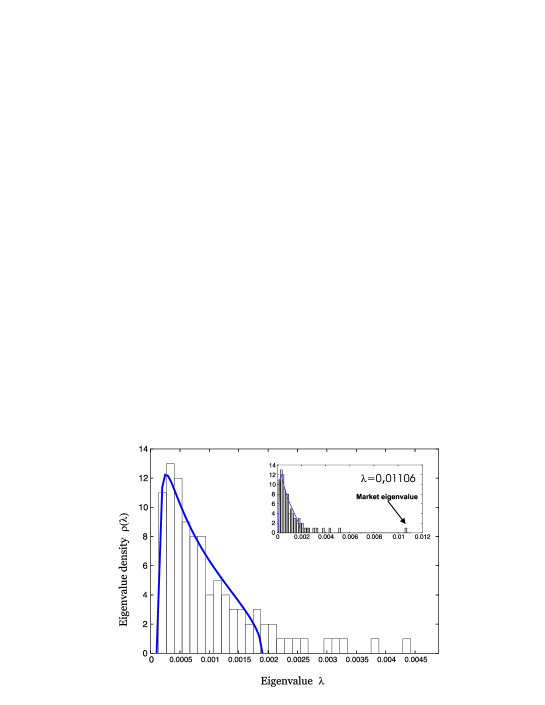
Figure 1: Histogram of eigenvalues for the WIG stocks from $29.01.1999$ till $17.01.2003$ with Wishart fit

If we look closely at Fig. 1 we can observe, that there are several large eigenvalues (the largest one is labeled as the market one, since it consists the information about all the stocks in the market i.e. is closely related to the WIG index), however the greater part of the spectrum is concentrated between $0$ and $0.002$ (i.e. The Wishart- fit ). We believe, that behind this Random part of the spectrum there exists single eigenvalue, which carries nontrivial and useful information. Exploiting the knowledge from Linear Algebra,we may rewrite our covariance matrix $\mathbf{Cov}$ as:

$$\mathbf{Cov=U\cdot D\cdot U^{T}}$$ (16)

Here $\mathbf{D}$ is a diagonal matrix of eigenvalues of the original matrix $\mathbf{Cov}$ and $\mathbf{U}$ is a matrix whose columns are normalized eigenvectors corresponding with proper eigenvalues. Furthermore $\mathbf{U}$ fulfills the equation:

$$\mathbf{U\cdot U^{T}=\mathrm{1}=U\cdot U^{-1}}$$ (17)

The trace is conserved, so we write:

$$\mathbf{Tr(Cov)=Tr(U\cdot D\cdot U^{T})}$$ (18)

Using the (17) and cyclic properties of the trace we get

$$\mathbf{Tr(D)=Tr(Cov)}$$ (19)

Following the fact, $\mathbf{D}$ is a diagonal matrix of eigenvalues one can decompose its trace in the following way:

$$\mathbf{Tr(Cov)}=\mathbf{Tr(D)}=\sum_{i}\lambda_{i}+\sum_{j}\lambda_{j}$$ (20)

where $\lambda_{i}\in[\lambda_{\min},\lambda_{\max}]$ is a set of eigenvalues that are predicted by (14) $\lambda_{j}\in[\lambda_{1},\lambda_{\min})\cup(\lambda_{\max},\lambda_{N}]$ is set of these eigenvalues, which do not obey the RMT conditions. If we now replace $\sum_{i}\lambda_{i}$ by one eigenvalue $\zeta$, we get

$$\zeta=\mathbf{Tr(Cov)}-\sum_{j}\lambda_{j}$$ (21)

This results in squeezing the Random part of the spectrum to a single degenerated eigenvalue. The diagonalized matrix has now only several eigenvalues.

2.3 Covariance Matrix Reconstruction

Due to noise - removing procedures we know exactly the eigenvalues of the real covariance matrix. But since we have no knowledge of the original covariance matrix, we do not have enough knowledge of it’s eigenvectors. The familiarity with of eigenvalues is not sufficient to find the covariance matrix.
After applying the denoising procedure we will reconstruct the covariance matrix using the diagonalized matrix with some eigenvalues shrinked and matrices of eigenvectors calculated for non-shrinked covariance matrix.
This reconstructed and unbiased Covariance Matrix is used as an initial Covariance Matrix in Markowitz Model described above. The new model itself is a part of automatic investing algorithm described in the next section. The results are presented in the last section.

3 An Overview of the System - Automatic Investing Algorithm

The Automatic Trading Agent is a client- server application for managing stock portfolios without involving user interference. It consists of three main parts: Virtual Agent, Data Collector and User Interface. Clients running the System on their workstations are able to monitor a stream of data (information about the state of a portfolio) from the ATA server using their web browsers. This part of application is controlled by the User Interface. In addition to different standard portfolio management tools ATA system includes several RMT - based techniques for building an optimal portfolio with the noise effect minimized.The system is designed not only to help a single client choose the right, optimal portfolio with a user-defined level of risk and expected return, but also to diminish user engagement in stock data and information analysis. Once the strategy is fixed, client is able to monitor the future changes in the portfolio; the rest including portfolio optimization, data picking, sending requests and buy / sell orders is done by a decision system - Virtual Agent.

Figure 2: The Architecture of the System

3.1 Database module and Data Collector

This part of the program is responsible for assembling and managing the stock data.It also verifies the database in accordance with the assets available for the transaction platform.

3.1.1 Database

The data are stored on the server as files with daily quotations in a separate folder. Any company is represented by a text file, whose name is the company’s ISIN number. Each file consist of two columns - one representing the dates and the second corresponding daily closing prices.

3.1.2 Data Collection

Data collector is a separate program run by the server each trading day, one hour after the daily quotations are closed. It downloads the current quotation from stock exchange data vendors (in our case http://www.parkiet.com) and writes it down into the database.
The matrix of stocks, which will be used in further portfolio analysis, is then filled with the data from the database.The algorithm loads all prices of securities for a certain time window from the previously defined folder.

3.1.3 Corrections Module

Data are sometimes corrupted during the transfer or from ’measurement’ reasons (i.e. there is no quotation for the certain stock and the Stock Exchange is unable to state the closing price). This result in imperfect and incomplete information and zeros in initial time series. The number of files may also vary, because it reflects the list of assets, which are currently available for trading.
This part of the program watches and controls the correctness of the files, the entries in the database and the number of files.

3.2 Virtual Agent

Virtual Agent is a specific decision-making system. It’s input are current and historical stock exchange information and data form the database. On output it generates specific requests and orders to transaction platform. In our case it is the Stock Exchange Game structure, based on the WARSET trading system.
Information conversion and data analysis is done one hour after WSE the session is closed. All new daily data are incorporated in the database and then optimal decision is taken and the sell/ buy request, which will be accomplished the next day, is sent.
The Virtual Agent build it’s resolutions on the Effective Portfolio Theory and Random Matrix Theory.

3.2.1 Covariance Matrix Module

This part of the systems offers various types of covariance matrix estimators, which are used in solution of Markowitz’s problem. The module’s default setting is the simplest Gaussian estimator (4), but this can be modified by the user. The Covariance Matrix Module is responsible for building a raw matrix from the data and also for reconstructing it after the denoising procedure.

3.2.2 Denoising and Filtering Module

The Module controls the diagonalization process, which uses the LU decomposition , i.e. calculation of eigenvalues and eigenvectors. The eigenvectors are stored in the system and the eigenvalues are used to reduce the degrees of freedom of the covariance matrix, as it is predicted by RMT. Default denoising procedure is the standard one, introduced by [1].

3.2.3 Portfolio optimization

This module is a separate program, which solves the Markowitz’s problem and finds the optimal portfolio and then sends buy / sell order. Before any request is sent, Virtual Agent verifies it’s own decisions using several criteria. The simplest one is to check, whether the costs of the predicted transaction are not higher, than the realized portfolio. If they are, then Agent sends hold request on the whole portfolio.
Such a portfolio correction is usually done once a month. . The correction means to find once again the portfolio with fixed level of return and risk accepted, regarding all the new quotations since the last accomplished correction.

3.2.4 Corrected Portfolio:

We have to compare two separate portfolios: the ’old’ one, which pattern is stored on the remote transaction platform with the ’new’ one, created using the incorporated quotations. The next step is to determine an abstract portfolio as a result of subtractions between the examined portfolios.
Let $\mathbf{n}$ is the vector of weights of the new portfolio, and $\mathbf{s}$ denotes the same vector for the old portfolio, then the weights of a correction one are:

$$\mathbf{w=n-s}$$ (22)

If a component of $\mathbf{w}$ is $<0$ the sell request is sent, and obviously for $w_{i}>0$ system performs a buy order.$w_{i}=0$ means system holds that certain asset and it’s share in a portfolio does not change.

3.2.5 Transaction costs:

Each change in a portfolio is charged with brockerages (Table: 1). To compensate this effect we need to sell slightly more individual stocks, than it arises from our analysis. The reverse effect has to be applied to buy request.

3.3 Communication and Reporting Modules - User interface

3.3.1 Communication Module

The communication module allows the Virtual Agent to connect to the Game platform and place appropriate orders. This module is a separate script, constructed to be independent of the trading platform. This gives the possibility to replace the Simulator used in the testing period by the real trading platform.

3.3.2 Reporting Module

The User Interface plays the role of the reporting module. It’s external part, accessible for the user is the web page (myricaria.if.uj.edu.pl). Here the investor can follow present information on accounts, the gains and losses figures and the history of all changes, investment strategies and decisions taken. The system user has also a possibility to change the key parameters of the program, such as investment strategy (choice of the level of risk accepted) and the frequency of portfolio corrections.

3.4 Implemented technologies

3.4.1 C# Language

The ATA is completely written in C# language, chosen because of multi-platform advantage. The programs may be written in one environment and then run under any platform i.e. Windows and Linux. the default environment for the ATA is linux server, but the programming process was made under Windows, so the multi-platform ability is a must.
Another important advantage of the language is the intuitive construction of mathematical formulas and the precision of calculations far beyond the popular C++ language, which in our case is crucial.

3.4.2 Linux Tools

The Data Collector is a BASH shell script, run by Cron daemon, every fixed number of days. The script also uses Wget to efficiently collect the data via FTP/HTTP. The AWK , SED and GREP allow the script very easily to explore and analyze high amounts of data.

3.4.3 HTML, PHP, CSS

The user interface is prepared as the website. The PHP scripts run by the www server Apache, allow the creation of dynamic HTML websites, where the content changes frequently. The proper view of the website in any internet viewer is controlled by the CSS.

4 Warsaw Stock Exchange Simulator and ATA implementation results

Here we present the results of the whole procedure described above. For our research we have chosen the Warsaw Stock Exchange simulator available via the world world wide web url http://gra.onet.pl, as a testground.

4.1 Rules of the game

There are several steps and rules a user must adhere and execute to properly use the simulator. First of all, the system needs to recognize us as its’ users, possessing so called onet_id. Thus the primary step is to register oneself in the onet system, by filling out a simple form. Using onet_id one may now log on http://gra.onet.pl to create our first account, with $40000$ PLN as an initial sum of money for every account. The number of accounts a single user may open is not limited and the money can be arbitrarily invested. Sharing more than one account number, one is able to check different investment strategies.
This game act like a real stock exchange and brockerage house. We have to start with buy order - choose financial instruments, which we want to buy and specify their quantity and price limits. If there are no constraints on price, then the order is realized at any price. All quotations are delayed $20$ minutes, to give the same chance to the players who cannot follow the quotations in real time. All orders are cancelable, also with $20$ minutes delay.Each user also has to pay transaction costs as in Table 1

Value of order	Height of brockerage
$\leq 500$ PLN	$10$ PLN
$500$–$2500$PLN	$10$PLN $+1,5\%$ over $500$ PLN
$2500$–$10000$PLN	$40$PLN $+1\%$ over $2500$ PLN
$\geq 10000$PLN	$115$PLN $+0,75\%$ over $10000$ PLN

Table 1: Costs and Commission (source: http://gra.onet.pl/nowa/prowizje.asp)

We have constructed a certain portfolio, after our buy order is being accomplished. Now we need to decide, what shares we need to buy / sell / hold to minimize the risk and maximize the return. To win an excellent rank and high gains, one need to be involved and follow the price changes permanently. Most of the steps one need to execute, except the choice of the accepted level of risk, can be done automatically by especially programmed virtual agent.

4.2 Data Selection and Analysis

The WIG index incorporates about $120$ stocks, which make about $80\%$ of all assets quoted during continuous trading. From our point of view, it is interesting to examine the connections (i.e. correlations) between these stocks.
In order to conduct further research and improve the effectiveness of our algorithm, we first need to identify and choose a stable period in the economy.

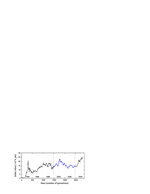
Figure 3: Changes in WIG index during the period from $1991$ till $2004$

We have related it with the period of the lowest volatility of the WIG index. We have started with the conversion of absolute changes of the WIG time series $S(t)$ to the relative ones according to

$$G(t)=\frac{S(t+1)-S(t)}{S(t)}$$ (23)

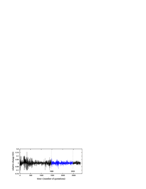
Figure 4: Fluctuations of relative WIG changes

Then for a fixed time window width $T=990$ quotations, the volatility of the time series $G(t)$ was calculated:

$$\sigma(t_{0})=\sqrt{\frac{1}{T-1}\sum_{i=0}^{T}\left(G(t_{0}+i)-\overline{G(T)}\right)^{2}}$$ (24)

where $\overline{G(T)}$ is the average $G(t)$ over the whole time window $T$.This results can be presented on the diagram:

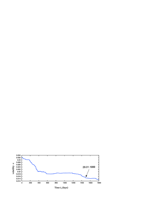
Figure 5: Volatility changes in time for a fixed window length

It is easy to notice, that first few years of quotations are determined by a relatively high volatility. That is why the period from $29.01.1999$ to $17.01.2003$ was chosen in further analysis and tests.
Another problem we have encountered during the analysis of historical data, was the incomplete information about some of $120$ stocks, which may result in the infinities in relative changes $G(t)$, when the lack of information was replaced by zeros in the original $S(t)$ time series . The separate ’zeros’ were extrapolated from the future and previous relative changes of a given time series. In the case, if more information is lost in the way, one is unable to predict the further prices then this stock is not very examined in further research. For the fixed period of $990$ days we have chosen then $100$ stocks and we have calculated the average standard deviation of price changes $\left\langle\sigma\right\rangle=0,4767$ and average correlation of returns between stocks $\left\langle corr_{ij}\right\rangle=0,0657$

Figure 6: Logarithmic price changes(on the left) and correlations (on the right) for WIG companies

4.3 Simulation on the historical data and it’s results

The next step in testing our system is to check how it works when the input and output data are historical. The selected time period was divided into parts. We have assumed, that the initial value of a portfolio is $40000$ PLN. We have used here a time window with variable width $T$. The analysis started with $T=139$ days. Every day, the $T$ - dimension of the matrix $\mathbf{M}$ was increased by one, until the final $T=849$ days.
The number of available stocks $N=100$ and the average number of stocks selected $45$. Every $316$ days the correction was made. The portfolio went to the roof on $151$ day with $56443,61$ PLN a a result. (This is $140\%$ of the initial value).
The portfolio went to the floor with $35042,66$ PLN after first $27$ days.
The result of the investment after $849$ days yields $47185,86$ PLN ,which means the $18\%$ gains compared to the $10\%$ WIG downfall.

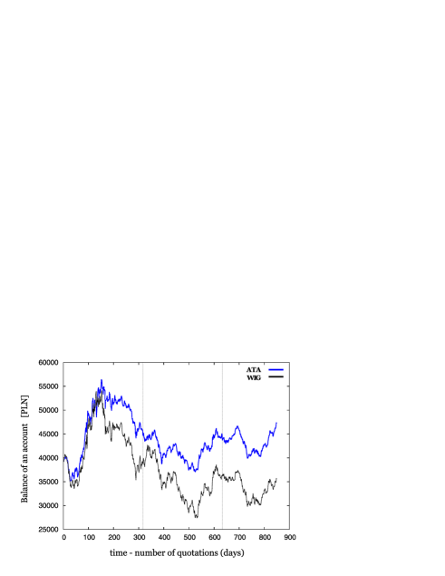
Figure 7: The Results of The Simulation on a Portofolio’s Balance. Vertical lines indicate the correction

Conclusions and Future Work

The aim of this paper was to introduce a simple RMT based mechanism, acting like an virtual trader in a portfolio selection and optimization process.Imposing the results from Random Matrix Theory our program reduces the statistical noise and gives a better estimation of future risk and return for a certain portfolio.However, in this paper only the simplest version of the programm was presented. An improvement of the program, which adopt it’s decisions to the all information available will be the part of our future work. From our point of view, an interesting for further analysis is the hypothesis, that there exist also time correlations between different shares. This fact might be useful in the detection of buy/ sell signals.

References

- [1] J.P.Bouchaud, M.Potters, Theory of Financial Risk. From Statistical Physics to Risk Management 2nd ed., Cambridge University Press, Cambridge 2003
- [2] Z. Burda, A. Görlich, A. Jarosz, J.Jurkiewicz, Signal and Noise in Correlation Matrix, http://arxiv.org/pdf/cond-mat/0305627
- [3] S.Chan, The Impact of Transaction Costs on Portfolio Optimization, Bachelor Thesis, Erasmus University, 2005
- [4] E.J.Elton, M.J.Gruber, Modern Portfolio Theory and Investment Analysis 6th ed., Wiley, New York 2002
- [5] T.Guhr, A.Müller - Groeling, H.A.Weidenmüller, Random matrix theories in quantum physics: common concepts, Phys. Rep. 299 (1998)
- [6] L.Laloux, P.Cizeau, J.P.Bouchaud and M. Potters, Noise Dressing of Financial Correlation Matrices, http://arxiv.org/pdf/cond-mat/9810255/
- [7] V.A. Marčenko, L.A. Pastur, Distribution of eigenvalues for some setes of random matrices, Math USSR Sbornik, 1: 457 -483 (1967)
- [8] Harry M.Markowitz ,Portfolio Selection, The Journal of Finance, Volume 7 No. 1, pp. 77-91 (1952)
- [9] Markus Rudolf, Algorithms for Portfolio Optimization and Portfolio Insurance,Verlag Paul Haupt, Bern, Stuttgart, Wien