Self-Consistent Asset Pricing Models

Abstract

We discuss the foundations of factor or regression models in the light of the self-consistency condition that the market portfolio (and more generally the risk factors) is (are) constituted of the assets whose returns it is (they are) supposed to explain. As already reported in several articles, self-consistency implies correlations between the return disturbances. As a consequence, the alpha’s and beta’s of the factor model are unobservable. Self-consistency leads to renormalized beta’s with zero effective alpha’s, which are observable with standard OLS regressions. When the conditions derived from internal consistency are not met, the model is necessarily incomplete, which means that some sources of risk cannot be replicated (or hedged) by a portfolio of stocks traded on the market, even for infinite economies. Analytical derivations and numerical simulations show that, for arbitrary choices of the proxy which are different from the true market portfolio, a modified linear regression holds with a non-zero value $\alpha_{i}$ at the origin between an asset $i$’s return and the proxy’s return. Self-consistency also introduces “orthogonality” and “normality” conditions linking the beta’s, alpha’s (as well as the residuals) and the weights of the proxy portfolio. Two diagnostics based on these orthogonality and normality conditions are implemented on a basket of 323 assets which have been components of the S&P500 in the period from Jan. 1990 to Feb. 2005. These two diagnostics show interesting departures from dynamical self-consistency starting about 2 years before the end of the Internet bubble. Assuming that the CAPM holds with the self-consistency condition, the OLS method automatically obeys the resulting orthogonality and normality conditions and therefore provides a simple way to self-consistently assess the parameters of the model by using proxy portfolios made only of the assets which are used in the CAPM regressions. Finally, the factor decomposition with the self-consistency condition derives a risk-factor decomposition in the multi-factor case which is identical to the principal components analysis (PCA), thus providing a direct link between model-driven and data-driven constructions of risk factors. This correspondence shows that PCA will therefore suffer from the same limitations as the CAPM and its multi-factor generalization, namely lack of out-of-sample explanatory power and predictability. In the multi-period context, the self-consistency conditions force the beta’s to be time-dependent with specific constraints.

1 Introduction

One of the most important achievements in financial economics is the Capital Asset Pricing Model (CAPM), which is probably still the most widely used approach to relative asset valuation. Its key idea is that the expected excess return of an asset is proportional to the expected covariance of the excess return of this asset with the excess return of the market portfolio. The proportionality coefficient measures the average relative risk aversion of investors. As a consequence, there is an irreducible risk component which cannot be diversified away, which cannot be eliminated through portfolio aggregation and thus has to be priced. The central testable implication of the CAPM is that assets must be priced so that the market portfolio is mean-variance efficient (Fama and French, 2004; Roll, 1977). However, past and recent tests have rejected the CAPM as a valid model of financial valuation. In particular, the Fama/French analysis (Fama and French, 1992; 1993) shows basically no support for the CAPM’s central result of a positive relation between expected return and global market risk (quantified by the beta parameter). In contrast, other variables, such as the market capitalization and the book-to-market ratio or the turnover and the past return, present some explanatory power.

More and more sophisticated extensions of the CAPM beyond the mean-variance approach have not improved the ability of the CAPM and its generalization to explain relative asset valuations. Let us mention the multi-moments CAPM, which has originally been proposed by Rubinstein (1973) and Krauss and Litzenberger (1976) to account for the departure of the returns distributions from Normality. The relevance of this class of models has been underlined by Lim (1989) and Harvey and Siddique (2000) who have tested the role of the asymmetry in the risk premium by accounting for the skewness of the distribution of returns and more recently by Fang and Lai (1997) and Hwang and Satchell (1999) who have introduced a four-moments CAPM to take into account the letpokurtic behavior of the assets return distributions. Many other extensions have been presented such as the VaR-CAPM (Alexander and Baptista, 2002), the Distributional-CAPM (Polimenis, 2005), and generalized CAPM models with consistent measures of risks and heterogeneous agents (Malevergne and Sornette, 2006a), in order to account more carefully for the risk perception of investors.

The arbitrage pricing theory (APT) provides an alternative to the CAPM. Like the CAPM, the APT assumes that only non-diversifiable risk is priced. But, unlike the CAPM which specifies returns as a linear function of only systematic risk, the APT is based on the well-known observations that multiple factors affect the observed time series of returns, such as industry factors, interest rates, exchange rates, real output, the money supply, aggregate consumption, investors confidence, oil prices, and many other variables (Ross, 1976; Roll and Ross, 1984; Roll, 1994). While observed asset prices respond to a wide variety of factors, there is much weaker evidence that equities with larger sensitivity to some factors give higher returns, as the APT requires. This weakness in the APT has led to further generalizations of factor models, such as the empirical Fama/French three factor model (Fama and French, 1995), which does not use an arbitrage condition anymore. Fama and French started with the observation that two classes of stocks show better returns that the average market: (1) stocks with small market capitalization (“small caps”) and (2) stocks with a high book-value-to-price ratio (often “value” stocks as opposed to “growth” stocks).

What then survive of the fundamental ideas underlying the CAPM? A key remark is that, given a set of assets, what is literally tested is the efficiency of a specific proxy for the market portfolio together with the CAPM. As recalled by Fama and French (2004), the CAPM requires using the market portfolio of all the invested wealth (which includes stocks, bonds, real-estate, commodities, etc.). More precisely, as first stressed by Roll (1977), “The theory is not testable unless the exact composition of the true market portfolio is known and used in the tests. This implies that the theory is not testable unless all individual assets are included in the sample.” (italics in Roll (1977)). Unfortunately, the market proxies used in empirical work are almost always restricted to common stocks, and as pointed out by Roll, the composition of a proxy for the market portfolio can cause quite confusing inferences on the validity of the test and the mean-variance efficiency of the market portfolio. It is thus possible that the CAPM holds, the true market portfolio is efficient, and empirical contradictions of the CAPM are due to bad proxies for the market portfolio. Given a universe of $N$ assets, it is always possible to construct a mean-variance portfolio (or any multi-moment generalization thereof), which will be such that the expected excess return of an asset is proportional to the expected covariance of the excess return of this asset with the excess return of the mean-variance portfolio. This results mechanically (or algebraically) from the construction of the mean-variance portfolio. While this property looks identical to the central test of the CAPM, in order for the CAPM to hold and for such a mean-variance portfolio to be the market portfolio, it should remain a mean-variance portfolio ex-ante (out-of-sample). The failure of the CAPM together with such a construction for the proxy of the market portfolio is revealed by the notorious instability of mean-variance portfolios (see for instance Michaud, 2003) with their weights needing to be continuously readjusted as a function of time. Empirically, the problem is that a mean-variance portfolio constructed over a given time interval will be no more in general a mean-variance portfolio (even allowing for a different average return) in the next period, and can not thus qualify as the market portfolio.

In addition to this problem of the market portfolio proxy, the “disturbances” in factor models are correlated, as a consequence of the self-consistency condition that, in a complete market, the market portfolio and, more generally, the explanatory factors are made of (or can be replicated by) the assets they are intended to explain (Fama, 1973) (see also Sharpe (1990)’s Nobel lecture). This presence of correlations between return residuals may a priori pose problems in the pricing of portfolio risks: only when the return residuals can be averaged out by diversification can one conclude that the only non-diversifiable risk of a portfolio is born by the contribution of the market portfolio which is weighted by the beta of the portfolio under consideration. Previous authors have suggested that this is indeed what happens in economies in the limit of a large market $N\to\infty$, for which the correlations between residuals vanish asymptotically and the self-consistency condition seems irrelevant. For example, while Sharpe (1990; footnote 13) concluded that, as a consequence of the self-consistency condition, at least two of the residuals, say $\varepsilon_{i}$ and $\varepsilon_{j}$, must be negatively correlated, he suggested that this problem may disappear in economies with infinitely many securities. In fact, we show in Malevergne and Sornette (2006b) that this apparently quite reasonable line of reasoning does not tell the whole story: even for economies with infinitely many securities, when the companies exhibit a large distribution of sizes as they do in reality, the self-consistency condition leads to the important consequence that the risk born out by an investor holding a well-diversified portfolio does not reduce to the market risk in the limit of a very large portfolio, as usually believed. A significant proportion of “specific risk” may remain which cannot be diversified away by a simple aggregation of a very large number of assets. Moreover, this non-diversifiable risk can be accounted for in the APT by an additional factor associated with the self-consistency condition.

Here, our more modest goal is to present a review of the foundation of factor models using the self-consistent condition as a pivot to organize the presentation and form threads across different results scattered in the literature. Our goal will be reached if the reader starts to appreciate, as the authors did in the course of their digestion of the literature leading to some new results reported in (Malevergne and Sornette, 2006b), the many subtle issues interconnecting the concepts of equilibrium, no-arbitrage and risk pricing. In the physicist language, these concepts describe ultimately what can probably be seen as the attractive fixed point (equilibrium) of self-organizing systems with feedbacks. We believe that the study of the inner-consistency of these models can be useful to inspire the development of novel approaches addressing the above issues and others.

The organization of the paper is the following. In the next section, we consider an equilibrium model where the assets return dynamics can be explained by a single factor, the market. At equilibrium, this model is consistent with the CAPM but, due to the self-consistency condition that the market portfolio is constituted of the assets whose returns it is supposed to explain, the parameters of the original factor model remain unobservable. Only the CAPM beta’s are observable if the true market portfolio is known. Due the self-consistency condition, the residuals of the regression of the assets’ returns with respect to the market portfolio can only be defined with a zero intercept. Then, the orthogonality condition obtained in Fama (1973) concerning the disturbances of the factor models is derived both for a one-factor as well as for a multi-factor model. In section 3, we discuss the calibration issues associated with the one factor model in relation with the impact of the non-observability of the actual market factor. We illustrate that, if a proxy is used (which is the real-life situation), then one can only measure a modified beta value which may differ from the true beta. In addition, a non-zero ‘alpha’ appears, which has however nothing to do with the unobservable alpha of the original factor model, but reflects the difference between the proxy and the market portfolio. Section 4 addresses the same question for multi-factor models. A multi-factor analysis with the self-consistency condition is shown to be equivalent to the principal component analysis (PCA) applied to baskets of assets. In the light of these results, section 5 offers a discussion of the theoretical and practical limitations of the factor-models. It underlines the necessity for the introduction of non constant $\beta$’s and propose some restrictions on the possible dynamics for the $\beta$. All the technical derivations are gathered in the 6 appendices.

2 Self-consistency of factor models

2.1 One-factor model: dynamical consistency of the CAPM

2.1.1 Factor model from CAPM

The celebrated Capital Asset Pricing Model, derived by Sharpe (1964), yields the famous relation known as the Market Security Line

$${\rm E}\left[r_{i}\right]=r_{0}+\beta_{i}\cdot{\rm E}\left[r_{m}-r_{0}\right],$$ (1)

where $r_{m}$, $r_{i}$ and $r_{0}$ denote the market return, the return on asset $i$ and the risk free interest rate respectively, while

$$\beta_{i}=\frac{{\rm Cov}~{}\left(r_{i},r_{m}\right)}{{\rm Var}~{}r_{m}}.$$ (2)

As stressed by Sharpe (1990), “the value $\beta_{i}$ can be given an interpretation similar to that found in regression analysis utilizing historic data, although in the context of the CAPM it is to be interpreted strictly as an ex-ante value based on probabilistic beliefs about future outcomes.” If the investors’ anticipations are self-fulfilling, the relationship between $r_{i}$ and $r_{m}$ can be modeled as

$$r_{i}=a_{i}+\beta_{i}\cdot r_{m}+\varepsilon_{i}~{},$$ (3)

with $a_{i}=\left(1-\beta_{i}\right)r_{0}$, provided that the expectation of the residual ${\rm E}\left[\varepsilon_{i}\right]$ is assumed to be zero. These two conditions $a_{i}=\left(1-\beta_{i}\right)r_{0}$ and ${\rm E}\left[\varepsilon_{i}\right]=0$ ensures that the market portfolio is efficient in the mean-variance sense. Indeed, taking expectations (or sample means) of (3), one obtains an exact linear cross-sectional relation between mean returns and beta’s. There is a one-to-one correspondence between exact linearity and mean/variance efficiency of the market portfolio (Bodie et al., 2004).

2.1.2 CAPM from a factor model

Let us now start from the opposite view point to determine the conditions under which the CAPM relation holds for an economy obeying a linear factor model, where the excess returns of asset prices over the risk-free rate $r_{0}$ are determined according to the following equation

$$\vec{r}_{t}=\vec{\alpha}+\vec{\beta}^{0}\cdot r_{m}(t)+\vec{\varepsilon}_{t},$$ (4)

where $\vec{r}_{t}$ is the $N\times 1$ vector of asset excess returns at time $t$, $r_{m}(t)$ is the excess return on the market portfolio and $\vec{\varepsilon}_{t}$ is a vector of disturbances with zero average ${\rm E}\left[\vec{\varepsilon}_{t}\right]=\vec{0}$ and covariance matrix $\Omega_{t}={\rm E}\left[\vec{\varepsilon}_{t}\cdot\vec{\varepsilon}_{t}^{\prime}\right]$. We assume that $\Omega_{t}$ is a deterministic function of $t$ and that the $\vec{\varepsilon}_{t}$ are independent. We do not make any other assumption concerning $\Omega_{t}$, in particular, we do not assume that it is a diagonal matrix since the CAPM places no restriction on the correlation between the disturbance terms. The symbols $\vec{\alpha}$ and $\vec{\beta}^{0}$ represent constant $N\times 1$ vectors.

Let us assume that the model (4) is common knowledge, i.e., each economic agent knows that the asset returns follow equation (4), each agent knows that all other agents know that the assets returns follow equation (4), and so on… Let us assume that, by reallocating her wealth $W_{t}$ among the $n$ risky assets and the risk-free asset at each intermediate time period $t=1,\ldots,T-1$, each agent aims at maximizing her expected terminal wealth $W_{T}$ under the constraint that its variance ${\rm Var}~{}W_{T}$ is not greater than a predetermined level $\sigma_{W_{T}}^{2}$. Mathematically, this dynamic optimization program reads

$$\quad~{}~{}\max_{\vec{w}}{\rm E}\left[W_{T}\right]$$

$$({\cal P}):\qquad {\rm s.t}~{}{\rm Var}~{}W_{T}\leq\sigma_{W_{T}}^{2}$$

$$\quad~{}~{}W_{t+1}=W_{t}\left[1+\vec{w}^{\prime}\vec{r}_{t}+r_{0}\right],\quad t=0,1,\ldots,T-1.$$

Many other approaches have been considered in the large body of literature devoted to the problem of optimal investment selection in a multi-period framework. In particular, the approaches based on the maximization of the expected utility of the terminal wealth or of the lifetime consumption seem to dominate, but they often rely on a specific choice of the utility function, such as the CARA, HARA or quadratic utility functions (Samuelson, 1969, Hakansson 1971, Pliska 1997, among many others). Since the choice of a particular utility function may appear as arbitrary, we have preferred to resort to the mean-variance criterion in so far as it constitutes a low order expansion approximation which holds irrespective of the specific form of the utility function.

The solution of problem $({\cal P})$ can be found for instance in Li and Ng (2000): at each time period $t$, the optimal strategy amounts to invest a fraction of wealth in the risk free asset and the remaining in the risky portfolio

$$\vec{w}_{t}^{*}=\frac{{\Sigma_{t}}^{-1}{\rm E}\left[\vec{r}_{t}\right]}{\vec{1}^{\prime}{\Sigma_{t}}^{-1}{\rm E}\left[\vec{r}_{t}\right]},$$ (6)

where $\Sigma_{t}={\rm Cov}~{}\vec{r}_{t}$ denotes the covariance of the vector of excess returns of the asset prices over the risk-free rate, at time $t$. As we shall see in the sequel, $\Sigma_{t}$ and ${\rm E}\left[\vec{r}_{t}\right]$ are known functions of $t$, which is a necessary assumption for the solution given by Li and Ng (2000) to hold.

Since all agents invest only in two funds, namely the risk-free asset and the risky portfolio with weights $\vec{w}^{*}_{t}$, if we assume that an equilibrium is reached at each time $t$, then the composition $\vec{w}^{*}_{t}$ of the risky portfolio must represent that of the market portfolio at time $t$. In other words, in full generality, $\vec{w}_{t}^{*}$ given by (6) is nothing but the efficient tangency portfolio on the frontier composed of the existing risky assets. It becomes the market portfolio of all assets when the assets being considered here comprise indeed all assets, which is the case we first examine. Section 3 discusses what happens when this is not the case. For the sake of simplicity, we will denote by $\vec{w}_{t}$ the composition of the market portfolio.

It is important to note that the result (6) holds irrespective of the time horizon $T$ chosen by the investors because the composition $\vec{w}_{t}$ of the market portfolio is independent of $T$. Only the relative part of wealth invested in the risk-free asset and in the market portfolio depends on $T$, but this has no effect on the composition $\vec{w}_{t}$ of the market portfolio. As a consequence, the result still holds when investors have different time horizons, as in real markets.

Now, accounting for the fact that the market factor is itself built upon the universe of assets that it is supposed to explain (which we refer to as the “self-consistent condition”), the model must fulfill the internal consistency condition

$$r_{m}(t)=\vec{w}_{t}^{\prime}\cdot\vec{r}_{t}.$$ (7)

Starting from this self-consistency condition together with the assumption that investors follow a dynamic mean-variance strategy and with the condition of market equilibrium, we show in Appendix A that the regression model (4) leads to the CAPM

$${\rm E}\left[\vec{r}_{t}\right]=\vec{\beta}_{t}{\rm E}\left[r_{m}(t)\right],$$ (8)

with

$$\vec{\beta}_{t}=\frac{{\rm Cov}~{}\left(\vec{r}_{t},r_{m}(t)\right)}{{\rm Var}~{}~{}r_{m}(t)}=\frac{\left(\vec{1}-\vec{\beta}^{0}\right)^{\prime}\Omega_{t}^{-1}\vec{\alpha}}{\vec{\alpha}^{\prime}\Omega_{t}^{-1}\vec{\alpha}}~{}\vec{\alpha}+\vec{\beta}^{0}~{}.$$ (9)

This shows that the regression model (4) is consistent with the relation of the CAPM provided that the internal consistency condition (7) holds together with the existence of an equilibrium.

The rather lengthly derivation in Appendix A is not needed in the standard approach in which the vector $\vec{\alpha}$ is identically zero and the market portfolio is mean-variance efficient as given by (6). Appendix A makes explicit that the parameters of the market model (4) are of no consequence for the CAPM. Appendix A derives the expression of the observable parameters of the CAPM (in particular the beta) from the parameters $\alpha$’s, $\beta_{0}$’s and the matrix $\Omega$ of the covariance of the disturbances $\vec{\varepsilon}$ of the market model.

Therefore, the general regression model (4) provides a reasonable statistical model to test the CAPM relation (8). But, two important point must be discussed. First, even if $\vec{\alpha}$ and $\vec{\beta}^{0}$ are assumed constant, the CAPM’s $\beta$ depends on time $t$ as soon as $\Omega_{t}$ is not constant. Thus, the heteroscedasticity of the residuals is sufficient to make the $\beta$’s time varying. Since, in the real market, the variance of assets returns is time varying (the so-called GARCH effect), one has to account for the dynamics of the $\beta$’s. Second, the equilibrium imposes a dynamic constraint on the composition of the market portfolio. On the one hand, it is endogenously determined by the investors’ anticipations according to formula (6). On the other hand, the market portfolio must be related to the market capitalization of each asset, which reflects the economic performance of the firms. Thus, the relation

$$w_{t+1}^{i}=w_{t}^{i}\cdot\frac{1+r_{t}^{i}+r_{0}}{1+r_{m}(t)+r_{0}}$$ (10)

must hold. The $r_{0}$ appears in the numerator and denominator because of our convention to denote by $r_{t}^{i}$ and $r_{m}(t)$ the excess returns of asset and market prices over the risk-free interest $r_{0}$. For the time being, we assume that this relation (10) is compatible with the dynamics described by (4) and with the optimal portfolio allocation (6) and will discuss this point in more detail at the end of this article.

2.2 One-factor model: observable parameters, orthogonality and normalization conditions

For ease of the exposition, let us assume that $\Omega_{t}$ remains constant during the time interval under consideration. As a consequence, $\vec{\beta}$ can be a priori independent of $t$ as shown by eq. (9), allowing us to remove the subscript $t$ in the sequel.

The previous sub-section has made clear that, according to (9), the coefficients $\vec{\beta}$ of the CAPM can be expressed in terms of the $\alpha$’s, $\beta_{0}$’s and the matrix $\Omega$ of the covariance of the disturbances $\vec{\varepsilon}$ of the market model. Actually, one can go further and show that the self-consistency condition implies that only $\vec{\beta}_{t}$ is observable while the coefficients $\vec{\alpha}$ and $\vec{\beta}^{0}$ are unobservable. Indeed, expression (4) cannot be directly calibrated by the OLS estimator since the disturbances $\vec{\varepsilon}_{t}$ are correlated with the regressors while an OLS estimation automatically construct residuals which are orthogonal to the factor decomposition. To see why the disturbances $\vec{\varepsilon}_{t}$ are correlated with the regressors $r_{m}(t)$, let us left-multiply expression (4) by $\vec{w}_{t}^{\prime}$. Then, the self-consistency condition (7) implies that

$$r_{m}(t)=\frac{{\vec{w}^{\prime}}_{t}\cdot\left(\vec{\alpha}+\vec{\varepsilon}_{t}\right)}{1-{\vec{w}^{\prime}}_{t}\cdot{\vec{\beta}}^{0}}~{},$$ (11)

unless $w_{t}\vec{\beta}^{0}=1$.

The fact that the regressors $r_{m}(t)$ are correlated with the residuals $\vec{\varepsilon}_{t}$ does not invalidate the OLS procedure. It just means that the OLS procedure will estimate residuals which are different from the model disturbances. The observed residuals are obtained by decomposing the disturbances $\vec{\varepsilon}_{t}$ on its component correlated with $r_{m}(t)$ plus a contribution uncorrelated with $r_{m}(t)$. We thus introduce two non-random vectors $\vec{\delta}$, $\vec{\gamma}$ and the random vector $\vec{u}_{t}$, uncorrelated with $r_{m}(t)$ with zero mean, such that

$$\vec{\varepsilon}_{t}=\vec{\delta}+\vec{\gamma}\cdot r_{m}(t)+\vec{u}_{t}.$$ (12)

Then, Appendix B shows that the one-factor model reduces to

$$\vec{r}_{t}=\vec{\beta}\cdot r_{m}(t)+\vec{u}_{t}~{},$$ (13)

with the “normalization” and ”orthogonality” conditions

$$\vec{w}_{t}^{\prime}\vec{\beta}=1~{}\quad{\rm and}\quad\vec{w}_{t}^{\prime}\vec{u}_{t}=0~{},$$ (14)

which derive from the self-consistency condition (7). The result (13) means that, under the assumption that $r_{m}(t)$ is observable, the OLS estimator of (4) provides an estimate of $\vec{\beta}$ and not of $\vec{\beta}^{0}$ and $\vec{\alpha}$ which remain unobservable. Taking the expectation of (13) recovers the CAPM prediction (8) as it should.

We should stress that the orthogonality condition $\vec{w}_{t}^{\prime}\vec{u}_{t}=0$ shows that at least two of the $u_{t,i}$ must be negatively correlated, which resemble Sharpe (1990)’s statement in his footnote 13. But, there is an important difference in that the regression (13) has zero intercept (its “alpha” is zero). The absence of intercept together with the mean-variance nature of the market portfolio automatically ensures the validity of the CAPM relation (8).

Using the jargon of physicists, we can rephrase these results as follows. The self-consistency condition together with the mean-variance efficient nature of the market portfolio imply that the market model (4) is “renormalized” into an observable model given by expression (13) with (14), that is, the “bare” parameters $\vec{\alpha}$ and ${\vec{\beta}}_{0}$ are renormalized into $\vec{0}$ and $\vec{\beta}$. A standard OLS regression (a measurement) gives access only to the renormalized values $\vec{0}$ and $\vec{\beta}$, in the same that physicists can only measure for instance the large scale renormalized mass and charge of an electron and not its bare values (Lifshitz et al., 1982).

2.3 Multi-factor model

Let us generalize (4) and assume that the excess return vector $\vec{r}_{t}$ of $n$ securities traded on the market (made of these $n$ assets), over the risk free interest rate, can be explained by the $q$-factor model

$$\vec{r}_{t} = \sum_{i=1}^{q}\vec{\beta}_{i}u_{i}(t)+\vec{\varepsilon}_{t},$$ (15)

$$= B\vec{u}(t)+\vec{\varepsilon}_{t},$$ (16)

where $B$ is the $n\times q$ matrix which stacks the vectors $\vec{\beta}_{i}$, $\vec{u}_{t}$ is the vector whose i^th component is the i^th risk factor $u_{i}$ and ${\rm E}\left[\vec{\varepsilon}(t)\right]=0$.

With $n$ assets and $n+q$ sources of randomness, the market is a priori incomplete. The market becomes complete if all risk factors can be replicated by an asset portfolio.

Consider the risk factor $i$, which can be replicated by the portfolio $\vec{w}_{i}$, that is, $u_{i}(t)=\vec{w}_{i}^{\prime}\vec{r}_{t}$ in vector notations. The internal consistency of the model implies that

$$\vec{w}_{i}^{\prime}\vec{r}_{t}=u_{i}(t)=\sum_{j=1}^{q}\left(\vec{w}_{i}^{\prime}\vec{\beta}_{j}\right)u_{j}(t)+\vec{w}_{i}^{\prime}\vec{\varepsilon}_{t},$$ (17)

so that

$$\sum_{j\neq i}\left(\vec{w}_{i}^{\prime}\vec{\beta}_{j}\right)u_{j}(t)+\left(\vec{w}_{i}^{\prime}\vec{\beta}_{i}-1\right)u_{i}(t)+\vec{w}_{i}^{\prime}\vec{\varepsilon}_{t}=0~{}.$$ (18)

For a complete market such that all the risk factors $u_{i}$’s can be replicated by asset portfolios $\vec{w}_{i}$’s, $i=1,\ldots,q$ and denoting by $W$ the matrix which stacks all the portfolio weight vectors $\vec{w}_{i}$’s, the self-consistency condition (18) generalizes into

$$\left({\rm Id}-W^{\prime}B\right)\vec{u}(t)=W^{\prime}\vec{\varepsilon}_{t}~{}.$$ (19)

Taking the expectation of both sides yields

$$\left({\rm Id}-W^{\prime}B\right){\rm E}\left[\vec{u}(t)\right]=0~{},$$ (20)

since we assume ${\rm E}\left[\vec{\varepsilon}(t)\right]=0$. Two cases must be considered.

• First case: $\det\left({\rm Id}-W^{\prime}B\right)\neq 0$ and the unique solution is ${\rm E}\left[\vec{u}(t)\right]=0$, so that ${\rm E}\left[\vec{r}_{t}\right]=0$ by (16), which does not capture a real economy.

• Second case: $\det\left({\rm Id}-W^{\prime}B\right)=0$, which means that the matrix $W^{\prime}B$ has rank $q-p$, for some $0<p\leq q$. Provided that the system admits a solution, this solution can be expressed as a linear combination of $p$ independent vectors. As a consequence, the expected excess return on each individual asset ${\rm E}\left[r_{i}\right]$ can be expressed as the linear combination of the expected value of only $p$ risk factors. Therefore, only $p$ factors really matter. This implies that, if we assume that assets excess returns really depend upon $p=q$ factors, the rank of the matrix $\left({\rm Id}-W^{\prime}B\right)$ should be $q-p=0$ so that the expectation of the excess return on each individual asset ${\rm E}\left[r_{i}\right]$ can be expressed as the linear combination of the expected value of all the $q$ risk factors. In such a case, we will say that the model is irreducible, an hypothesis that we will assume to hold in the sequel. The case $p<q$ can be treated analogously by expressing the excess return of each individual asset as a linear combination of the expected value of the $p$ risk factors.

The condition that the rank of the matrix $\left({\rm Id}-W^{\prime}B\right)$ should be zero for the asset excess returns to depend on the $q$ irreducible factors simply means that the normalization condition

$$W^{\prime}B={\rm Id}$$ (21)

must hold. This relation is satisfied by the market factor in the CAPM, and generalizes the normalization condition discussed in section 2.1. In addition, equation (19) together with (21) enables us to conclude that

$$W^{\prime}\vec{\varepsilon}_{t}=0~{},$$ (22)

which means that the vector $\vec{\varepsilon}_{t}$ of disturbances has dimension $n-q$ at most, provided that $W$ is full rank, i.e. provided that the $q$ risk factors $u_{i}(t)$ can be replicated by $q$ linearly independent portfolios $\vec{w}_{i}$. Condition (22) generalizes the orthogonality condition for the one-factor model derive in section 2.2. The two conditions (21) and (22) generalize the orthogonality and normalization conditions (14) obtained for the one-factor CAPM.

Note that $\vec{u}$ and $\vec{\varepsilon}$ are uncorrelated under the condition that the $q$ risk factors $u_{i}(t)$ can be replicated by $q$ linearly independent portfolios.

To sum up, the possibility to replicate the risk factors by portfolios implies strong internal consistency conditions for factor models, namely equations (21) and (22). Conversely, if these conditions are not met, the model is necessarily incomplete, which means that some sources of risk cannot be replicated (or hedged) by an asset portfolio. Therefore, risk factors, such as the GDP, the term spread, the dividend yield, the size and book-to-market factors (Fama and French, 1993; 1995) and so on, could bring in additional information with respect to the usual market factor. See Petkova (2006) for empirical evidence.

3 Non-observability of the market portfolio (One-factor model)

3.1 What if the proxy is different from the true market portfolio?

In practice, the true market factor is unknown and one commonly uses a proxy. We show in Appendix C that model (13) leads to

$$\vec{r}_{t}=\underbrace{\left({\rm E}\left[r_{m}\right]\vec{\beta}-{\rm E}\left[\tilde{r}_{t}\right]\vec{\tilde{\beta}}\right)}_{\vec{\tilde{\alpha}}}+\vec{\tilde{\beta}}\cdot\tilde{r}_{t}+\vec{\eta}_{t}~{},$$ (23)

where $\tilde{r}_{t}$ is the proxy excess return, $\vec{\tilde{\beta}}$ is the vector of beta’s of the regression of asset excess returns on the proxy and $\vec{\eta}_{t}$ has zero mean ${\rm E}\left[\vec{\eta}_{t}\right]=0$ and is uncorrelated with the proxy ${\rm Cov}~{}\left(\vec{\eta},\tilde{r}_{t}\right)=0$. The explicit dependence of $\vec{\tilde{\beta}}$ as a function of the true $\vec{\beta}$, the weights $\tilde{w}_{t}^{\prime}$ of the portfolio proxy, the variance ${\rm Var}r_{m}$ of the market portfolio excess returns and the covariance matrix $\tilde{\Omega}$ of the vector $\vec{u}_{t}$ of residuals of the model (13) is given in equation (85).

The result (23) derives straightforwardly from the CAPM formulated explicitly with (13) and (14) by again using a self-consistent (or endogenous) condition that the proxy is itself a portfolio of the assets it is supposed to explain. As a consequence of the internal consistency requirement, one gets new orthogonality and normalization conditions. As previously, we have the normalization and orthogonality conditions

$$\tilde{w}_{t}^{\prime}\vec{\tilde{\beta}}=1,\quad{\rm and}\quad\tilde{w}_{t}^{\prime}\vec{\eta}_{t}=0,$$ (24)

where $\tilde{w}_{t}$ represents the composition of the proxy at time $t$. In addition, we have the following orthogonality constraint

$$\tilde{w}_{t}^{\prime}\vec{\tilde{\alpha}} = \tilde{w}_{t}^{\prime}\left({\rm E}\left[r_{m}\right]\vec{\beta}-{\rm E}\left[\tilde{r}_{t}\right]\vec{\tilde{\beta}}\right),$$ (25)

$$= \underbrace{\left(\tilde{w}^{\prime}\vec{\beta}\right)}_{\beta~{}{\rm of~{}the~{}proxy}}\cdot{\rm E}\left[r_{m}\right]-{\rm E}\left[\tilde{r}_{t}\right],$$

$$= 0~{},$$

provided that the CAPM relation holds.

Using a proxy instead of the true market portfolio yields a non-vanishing intercept $\vec{\tilde{\alpha}}={\rm E}\left[r_{m}\right]\vec{\beta}-{\rm E}\left[\tilde{r}_{t}\right]\vec{\tilde{\beta}}$ in the regression of the excess returns of each asset as a function of the excess returns of the portfolio proxy, which is a priori different from asset to asset. However, taking the expectation of (23), we obtain

$${\rm E}\left[r_{i,t}\right]={\rm E}\left[r_{m}\right]\beta_{i}=\left({{\rm E}\left[r_{m}\right]\over{\rm E}\left[\tilde{r}_{t}\right]}{\beta_{i}\over{\tilde{\beta}}_{i}}\right){\rm E}\left[\tilde{r}_{t}\right]~{}\tilde{\beta}_{i}~{},$$ (26)

for each individual asset $i$. As in the standard CAPM prediction, we thus obtain that the expected excess return ${\rm E}\left[\vec{r}_{i,t}\right]$ of an asset $i$ is proportional to its beta ${\tilde{\beta}}_{i}$ (obtained from the conditional regression (23)). But there is a major difference with the standard CAPM prediction, which is that the coefficient of proportionality is not simply the expectation ${\rm E}\left[\tilde{r}_{t}\right]$ of the proxy excess returns (as one could expect naively from translating the standard result to the proxy case). The difference involves the two correction factors ${\rm E}\left[r_{m}\right]/{\rm E}\left[\tilde{r}_{t}\right]$ and $\beta_{i}/\tilde{\beta}_{i}$, the second one being non-constant since it is a function of $\tilde{\beta}_{i}$ itself. Recall that ${\rm E}\left[r_{m}\right]$ and the $\beta_{i}$’s are in principle unobservable. We can thus expect a deviation from the standard CAPM linear relationship due to an increased scatter induced by the scatter in the coefficient of proportionality between expected excess return and beta evaluated with a market proxy.

Although this result is generally true, there is an exception. If the proxy happens to be on the ex-ante mean/variance efficient frontier, there will be an exact cross-sectional relation between expected returns and betas (calculated against the proxy) and there will be no scatter around the linear relation between mean returns and beta’s. Any market proxy will produce exact linearity, not just the tangency portfolio from the translated (by $r_{0}$) origin. Of course, the beta’s will be different for each such proxy but there will be no scatter. Generally, there is no need to assume the existence of a riskless rate. This is the heart of Black (1972)’s generalization of the CAPM. If there is no riskless rate, any ex-ante mean-variance efficient portfolio, which can lie anywhere on the positive or negative part of the frontier, will produce exact cross-sectional mean return/beta linearity. The only exception is the global minimum variance portfolio, which is positively correlated with all assets. For all other market proxies, there is a “zero-beta” portfolio, a portfolio uncorrelated with the chosen proxy, which serves in place of the riskless rate.

3.2 Empirical illustration

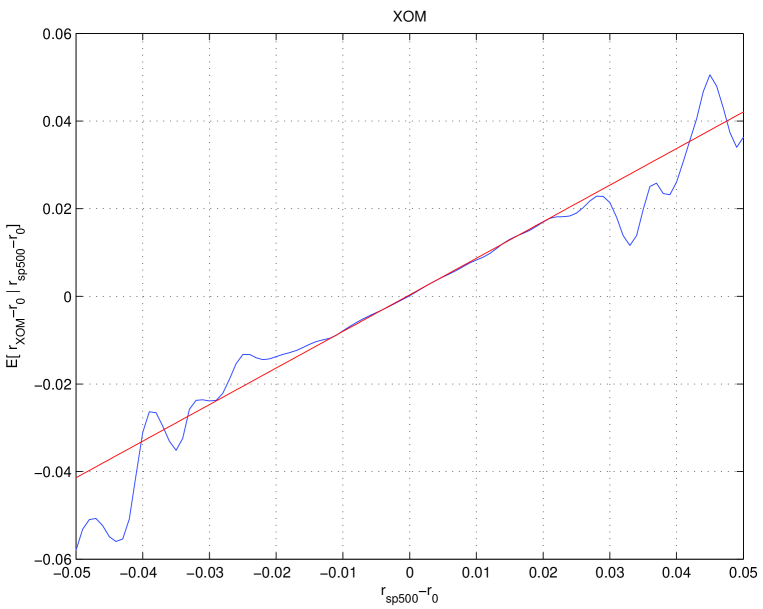
Figure 1: Regression of the expected return above the risk-free interest rate for Exxon mobil daily returns with respect to the excess return of the S&P500 index over the period from July 1962 to December 2000. The risk free interest rate is obtained from the three month Treasury Bill.

As an illustration, let us first take the S&P500 index as a proxy for the USA market portfolio. Figure 1 shows the average daily return of Exxon mobil (ticker XOM) daily returns conditioned on a fixed value of the S&P500 index daily returns $r_{m}(t)$ over the period from July 1962 to December 2000. In practice, we consider a given value $r_{m}$ (to within a small interval) of the S&P500. We then search for all days for which the return of the S&P500 was equal to this value $r_{m}$ (to within a small interval). We then take the average of the daily return of Exxon mobil realized in all these days. We then iterate by scanning all possible values of $r_{m}$ and use a kernel estimation to get a smoother and more robust estimation. Note that this procedure is non-parametric and provides an interesting determination of the market model. Indeed, suppose that the return $r_{i}$ of an asset $i$ is given by

$$r_{i}(t)=F_{i}[r_{m}(t)]+e(t)~{},$$ (27)

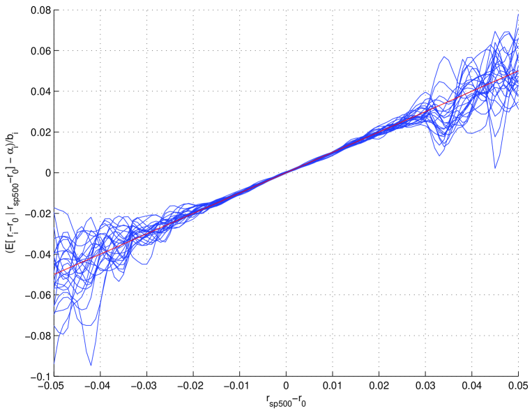
Figure 2: Each curve is similar to that shown in figure 1 and represents the normalized expected return above the risk-free interest rate defined by (30) for a given stock $i$ over the period from July 1962 to December 2000 as a function of the excess return $r_{SP500}-r_{0}$ above the risk-free interest rate $r_{0}$ of the S&P500 index taken as a proxy of the market portfolio. Since the $\alpha_{i}$’s and $\beta_{i}$’s are different from asset to asset, the normalization (30) ensures by construction that a good linear regression for each asset should be qualified by having all curves collapse on the diagonal, with unit slope and crossing of the origin, as observed up to statistical fluctuations. The 25 curves corresponds to the following stocks: Abbott Laboratories, American Home Products Corp., Boeing Co., Bristol-Myers Squibb Co., Chevron Corp., Du Pont (E.I.) de Nemours & Co., Disney (Walt) Co., General Electric Co., General Motors Corp., Hewlett-Packard Co., International Business Machines Co., Coca-Cola Co., Minnesota Mining & MFG Co., Philip Morris Cos Inc., Merck & Co Inc., Pepsico Inc., Pfizer Inc., Procter & Gamble Co., Pharmacia Corp., Schering-Plough Corp., Texaco Inc., Texas Instruments Inc., United Technologies Corp., Walgreen Co. and Exxon Mobil Co. The risk free interest rate is obtained from the three month Treasury Bill.

where $F_{i}[x]$ is an a priori arbitrary (possibly non-linear function) and $e(t)$ are the zero-mean residuals. Then, the above non-parametric procedure (whose result is shown in figures 1 and 2) amounts to calculate ${\rm E}[r_{i}|r_{m}=x]$ as a function of $x$:

$${\rm E}[r_{i}|r_{m}=x]=F_{i}[x]~{}.$$ (28)

Figure 1 plots the function $F_{i}[x]$ determined non-parametrically from the data. It seems that a linear dependence proves a reasonable approximation of the data presented in Fig. 1. The straight line is the line of equation $y=\alpha_{\rm XOM}+\beta_{\rm XOM}\cdot r_{SP500}(t)$, where $\beta_{\rm XOM}$ is obtained from the regression

$$r_{\rm XOM}(t)=\alpha_{\rm XOM}+\beta_{\rm XOM}\cdot r_{SP500}(t)+\varepsilon_{\rm XOM}(t)$$ (29)

of the returns.

This plot presented in Fig. 1 is typical of the relationship between conditional expected returns as a function of the return of the S&P500 index, obtained for all stocks in the S&P500, as shown from the superposed data in figure 2. Figure 2 is the same as figure 1, but for 25 different assets. In order to represent the corresponding functions $F_{i}(x)$ for each asset on a same figure without loosing visibility, we have just translated and scaled each curve, i.e., we plot

$$\frac{{\rm E}\left[r_{i}-r_{0}|r_{SP500}-r_{0}\right]-\alpha_{i}}{\beta_{i}}=(F_{i}[x]-\alpha_{i})/\beta_{i}~{},$$ (30)

as a function of $x=r_{SP500}-r_{0}$, where the $\alpha_{i}$’s and $\beta_{i}$’s are obtained by linear regressions similar to (29), one fit being performed for each non-parametrically determined $F_{i}$. The risk-free interest rate $r_{0}$ is basically negligible at the daily scale. ${\rm E}\left[r_{i}-r_{0}|r_{SP500}-r_{0}\right]$ is the expected return of stock $i$ above the risk-free interest rate, conditional on the value of $r_{SP500}-r_{0}$. The straight line in Figure 2 has slope $1$ and goes through the origin, thus confirming the remarkable quality of the relationship between the conditional expected asset returns and the S&P500 index daily returns, in agreement with (23). In other words, Figure 2 seems to confirm that the $F_{i}$’s appear to be quite closely approximated by an affine function: $F_{i}[x]=\alpha_{i}+\beta_{i}x$.

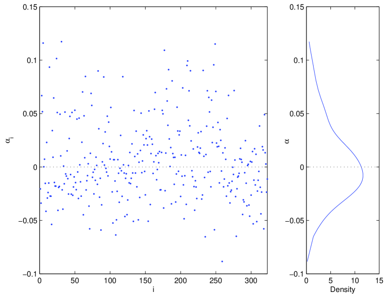
Figure 3: Left panel: Population of the intercepts of the regression of the expected monthly excess returns of 323 stocks entering into the composition of the S&P500 between January 1990 and February 2005 versus the monthly excess returns of the effective S&P323 index that we have constructed as a portfolio of these 323 stocks with weights proportional to their capitalizations. The risk free interest rate is obtained from the three month Treasury Bill. The abscissa is an arbitrary indexing of the 323 assets. The estimated probability density function of the population of alpha’s is shown on the right panel and illustrates the existence of a systematic bias for the alpha’s.

We have performed similar regressions as a function of the S&P500 returns for the monthly returns of the 323 stocks which remained into the composition of the S&P500 over the period between January 1990 and February 2005. But, in order to test the self-consistency condition and its consequences derived above, one could argue that it should be better to construct a market portfolio based solely on these 323 stocks. We have thus constructed an effective S&P323 index, constituted as a portfolio of these 323 stocks with weights proportional to their capitalizations. The regressions of the expected monthly returns of each of these 323 stocks conditioned on the S&P323 index monthly returns as a function of the S&P323 index monthly returns are similar to those obtained on the S&P500 and resemble the regressions shown in figures 1 and 2 albeit with more noise (not shown). Figure 3 shows the population of the intercepts (the alpha’s) of these regression. The abscissa is an arbitrary indexing of the 323 assets. The estimated probability density function of the population of alpha’s is shown on the right panel and illustrates the existence of a systematic bias for the alpha’s, as expected from the previous section 3.1. Note that the bias is negative which reflects the fact that over the period of study, the average performance of the S&P323 (and even more so for the S&P500) has been smaller than the risk-free rate. Another way of formulating the existence of the bias is just to say that the constructed index is not located on the sample efficient frontier.

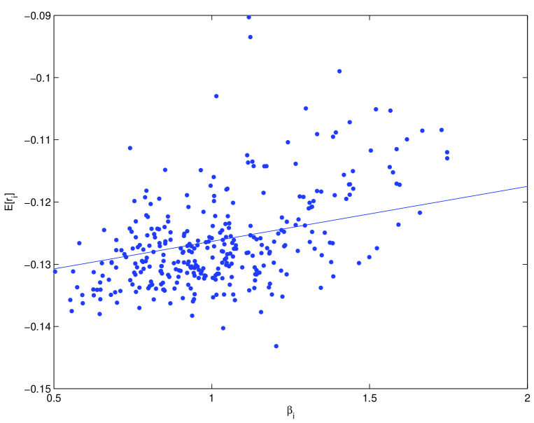
Figure 4: Expectation ${\rm E}\left[r_{i}-r_{0}\right]$ of the monthly excess returns of the 323 assets used in figure 3 as a function of their $\beta_{i}$ obtained by regressions with respect to the excess return to the effective S&P323 index. The risk free interest rate is obtained from the three month Treasury Bill. Under the CAPM hypothesis, one should obtain a straight line with slope ${\rm E}\left[r_{SP323}-r_{0}\right]$ ($-13.1\%$ per month) and zero additive coefficient at the origin. The straight line is the regression $y=0.88\%-13.5\%\cdot x$.

Figure 4 plots the expected returns ${\rm E}\left[r_{i}-r_{0}\right]$ of the monthly excess returns of the 323 assets used in figure 3 as a function of their $\beta_{i}$ obtained by regressions with respect to the excess return to the effective S&P323 index. Under the CAPM hypothesis, one should obtain a straight line with slope ${\rm E}\left[r_{SP323}-r_{0}\right]$ ($-13.1\%$ per month) and zero additive coefficient at the origin. The straight line is the regression $y=0.88\%-13.5\%\cdot x$. A standard statistical test shows that the value $0.88\%$ of the intercept at the origin is not statistically significant from zero. Together with the reasonable agreement between the slope of the regression and the excess expected returns of the S&P323 index, this would give a positive score for the CAPM. This is perhaps surprising considering the biases distribution of alpha’s shown in figure 3. This suggests that this standard expected return/beta tests examplified in figure 3 has not large power.

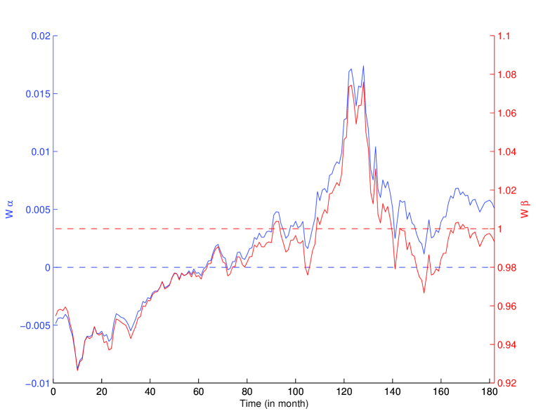
Figure 5: Time evolution of $\tilde{w}_{t}^{\prime}\vec{\tilde{\beta}}$ (red and right vertical scale) and $\tilde{w}_{t}^{\prime}\vec{\tilde{\alpha}}$ (blue and left vertical scale) over the period from January 1990 to February 2005 which includes 182 monthly values. $\tilde{w}_{t}$ is the vector of weights of the 323 stocks in our effective S&P323 index which evolves at each time step according to the capitation of each stock. $\vec{\tilde{\beta}}$ and $\vec{\tilde{\alpha}}$ are the two vectors of beta’s and alpha’s obtained from the regressions used in figures 3 and 4. According to the self-consistency conditions (24) and (25), the dynamical consistency of the CAPM should lead to $\tilde{w}_{t}^{\prime}\vec{\tilde{\beta}}=1$ and $\tilde{w}_{t}^{\prime}\vec{\tilde{\alpha}}=0$ at all time periods.

As a complement, one can use the self-consistency conditions $\tilde{w}_{t}^{\prime}\vec{\tilde{\beta}}=1$ (expression 24) and $\tilde{w}_{t}^{\prime}\vec{\tilde{\alpha}}=0$ (expression 25) to perform empirical tests. As explained in section 2.1, the dynamical consistency of the CAPM imposes that these two relationships should hold at each time step for the proxy of the market portfolio. We have thus calculated $\tilde{w}_{t}^{\prime}\vec{\tilde{\beta}}$ and $\tilde{w}_{t}^{\prime}\vec{\tilde{\alpha}}$, where $\tilde{w}_{t}$ is the vector of weights of the 323 stocks in our effective S&P323 index which evolves at each time step according to the capitation of each stock while $\vec{\tilde{\beta}}$ and $\vec{\tilde{\alpha}}$ are the two vectors of beta’s and alpha’s obtained from the regressions used in figures 3 and 4. Figure 5 shows the time evolution of $\tilde{w}_{t}^{\prime}\vec{\tilde{\beta}}$ and $\tilde{w}_{t}^{\prime}\vec{\tilde{\alpha}}$ over the period from January 1990 to February 2005 which includes 182 monthly values. The deviations respectively from $1$ and $0$ are significant, as shown by a standard Fisher test. The close connection between the time varying average alpha and beta shown in Figure 5 results from their common dynamics through the evolution of the weights $\vec{w}$.

The variable $\tilde{w}_{t}^{\prime}\vec{\tilde{\beta}}$ can be interpreted as the average beta of the stocks in the self-consistent market proxy. A value different from $1$ suggests that the market is out of equilibrium. In particular, if $\tilde{w}_{t}^{\prime}\vec{\tilde{\beta}}>1$, this can be interpreted as an “over-heating” of the market with the existence of positive feedback. Interestingly, this occurs just about two years before the peak of the Internet bubble in April 2000. It then took about two years after the peak to recover an equilibrium. Since early 2003, the market seems to have remained approximately at equilibrium according to this metric.

3.3 Tests on a synthetically generated market

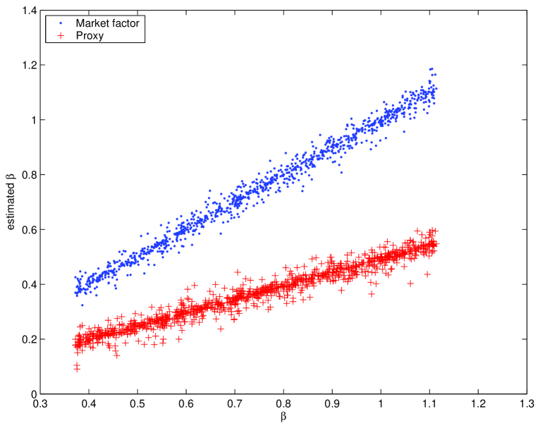
Figure 6: Synthetic tests on an artificial market of 1000 synthetic assets with properties adjusted to mimic those of the real US market. The plot shows the estimated beta’s obtained from the regression of the asset returns on the returns of the market portfolio (blue dots) and on the returns of the proxy (red crosses), as a function of the true beta’s. The upper straight line corresponds to the ideal case where the estimated beta’s equal the true beta’s. The lower straight line is the predicted dependence (85) of the beta’s estimated with the proxy as a function of the true beta.

In order to investigate the sensitivity of these tests, and in particular the impact of using a proxy for the market portfolio, we have constructed a toy (synthetic) market in which 1000 assets are traded and such that their returns at time $t$ obey equation (13) with the constraints (14). The weight of each asset in the market portfolio is drawn from a power law with tail index equal to one, in accordance with empirical observations on the distribution of firm sizes (Axtell, 2001), and then renormalized so that the weights sum up to one. For the purpose of illustration and easiness in testing, we impose that the composition of the market remain constant, i.e., the economy is stationary. The interest in this condition is that we can then study the pure impact of not observing the true market but only the proxy constructed on a subset of the whole universe of assets. The daily return on the synthetic market factor follows a Gaussian law with mean and standard deviation equal to the mean and the standard deviation of the daily return on the S&P500 over the time period from July 1962 to December 2000, namely $0.037\%$ and $0.90\%$ respectively. The $\beta$’s are also randomly drawn from a uniform law with mean equals to one and are such that they satisfy the normalization condition (14). It can be seen in figure 6 that the $\beta$’s range between $0.35$ and $1.15$, which is reasonable if we refer to the values usually reported in the literature. Finally, the residuals $\vec{\varepsilon}_{t}$ are drawn from a degenerate multivariate Gaussian distribution (i.e., the rank of its covariance matrix is $N-1=999$), so that they fulfill the orthogonality condition (14). The variances and covariances of these residuals have been fixed in such a way that they are of the same order of magnitude as the variances and covariances of the residuals estimated by linear regression of our basket of 25 assets on the S&P500. Thus, the values given by our toy market are expected to be consistent with the values observed on the actual market if the description by a one factor model has some merit.

Using the OLS estimator, we have first performed a regression with respect to the true market portfolio, whose composition is assumed to remain constant as we said. Then, we have constructed an arbitrary portfolio and have considered it to be the proxy of the market portfolio. We have then performed the linear regression of the assets returns on the proxy returns. Figure 6 compares the estimated beta’s obtained from the regression of the asset returns on the returns of the market portfolio with those obtained from the regression on the returns of the proxy, as a function of the true beta’s. The regression on the market factor gives a line with unit slope and zero intercept, as expected from the construction of the synthetic market. The regression on the proxy returns gives also a straight line, as predicted from the linear relation between $\vec{\beta}$ and $\vec{\tilde{\beta}}$ given by (85) in Appendix C. Figure 6 provides a verification of the properties put by construction in our synthetic market. Obviously, no one would be able to perform this verification on real data since the market portfolio and thus the true beta’s are unknowable.

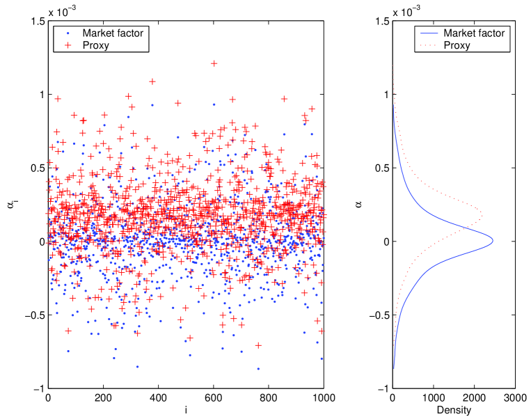
Figure 7: Synthetic tests on an artificial market of 1000 synthetic assets with properties adjusted to mimic those of the real US market. Left panel: Population of the intercepts of the regression of expected stock returns versus the market return (blue dots) or versus the proxy return (red crosses) in our synthetic market. The abscissa is an arbitrary indexing of the 1000 assets of our artificial market. The estimated probability density functions of the two population of alpha’s are shown on the right panel and illustrate the existence of a systematic bias for the proxy’s alpha’s.

Figure 7 shows the population of the intercepts of the regression of expected stock returns versus the market return or versus the proxy return in our synthetic market. These intercepts are presented as a function of the (arbitrary) indices of the 1000 assets. For the regression on the market factor, one can observe as expected a scatter around zero. For the regression on the market proxy, the intercepts are, on average, all significantly different from zero. As expected, the orthogonality and normalization conditions $\tilde{w}^{\prime}\vec{\alpha}=0$ and $\tilde{w}^{\prime}\vec{\tilde{\beta}}=1$ are satisfied, providing a verification of the validity of the numerical implementation of the model for these synthetically generated data. Thus, figure 7 confirms that a universe of assets which by construction obeys the CAPM exhibits non-zero alpha intercepts (which take apparently random values) when using an arbitrary proxy. This result can be compared with the empirical analog shown in figure 3.

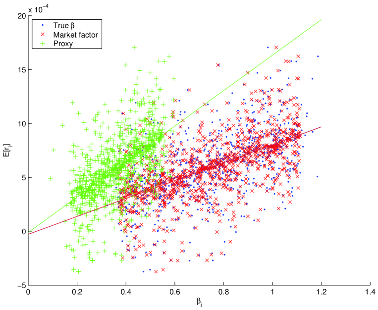
Figure 8: Synthetic tests on an artificial market of 1000 synthetic assets with properties adjusted to mimic those of the real US market. Individual expected returns ${\rm E}\left[r_{i}\right]$ for each of the 1000 assets (i) as a function of the true $\beta_{i}$’s (blue dots), (ii) as a function of the $\beta_{i}$’s obtained by regression on the true market (red crosses $\times$) and by regression on the proxy (green $+$). The straight lines are the linear regressions.

Figure 8 shows the individual expected returns ${\rm E}\left[r_{i}\right]$ for each of the 1000 assets (i) as a function of the true $\beta_{i}$’s, (ii) as a function of the $\beta_{i}$’s obtained by regression on the true market and (iii) by regression on the proxy. As expected, the dependence of the expected returns on the true beta’s and on the beta’s obtained from the true market portfolio follows the CAPM prediction, but with rather significant fluctuations. The scatter of the dependence of the expected returns on the beta’s determined from the proxy is larger but one can still observe a well-defined linear dependence with a zero intercept, and a slope different from the expected return ${\rm E}\left[\tilde{r}_{t}\right]$ of the portfolio proxy, as predicted in expression (26). This seems to justify why the bias in the distribution of alpha’s does not seem to affect the existence of the standard expected return/beta test shown in figure 3.

3.4 On the orthogonality and normality conditions

To summarize, the condition of self-consistency leads to the orthogonality and normality conditions (14) for the mono-factor model and to (21,22) for the multifactor model when the market portfolio is known. The orthogonality and normality conditions still hold when only a market proxy is available and they take the form (24) together with the additional orthogonality constraint (25). This suggests to use the orthogonality and normality conditions as new tests of the CAPM in the real-life situation where the market portfolio is not known and a somewhat arbitrary proxy is used. The motivation of these tests stems from the fact that they are not affected by the problem of using a proxy which is different from the real market factor, in contrast with the problem on the standard test of the CAPM made explicit in figure 8. Concretely, this suggests to complement the standard expected excess return versus beta, by tests checking the validity of the orthogonality and normality conditions when using for the proxy, not the S&P500, but any portfolio constructed on the assets used in the test. A test of the CAPM would then consist in testing the normalization and orthogonality conditions (24-25), which should hold for any such proxy portfolio.

It turns out however that the OLS estimated intercepts $\hat{\vec{\alpha}}$, the estimated $\beta$’s $\hat{\vec{\beta}}$ and the estimated residuals $\hat{\vec{\eta}}$ of a basket of assets necessarily satisfy the constraints (24-25) when the proxy used as the regressor is a portfolio build on these same assets. Let us denote by $Y$ the matrix which stacks the returns of the basket of the $N$ assets under consideration, by $X$ the matrix of the regressors, by $B$ the matrix of the regression coefficients and by $U$ the matrix which stacks the vectors of the residuals:

$$Y=\left(\begin{array}[]{c}{\vec{r}_{1}}^{\prime}\\ \vdots\\ {\vec{r}_{T}}^{\prime}\end{array}\right),\quad X=\left(\begin{array}[]{cc}1&r_{m}(1)\\ \vdots&\vdots\\ 1&r_{m}(T)\end{array}\right),\quad B=\left(\begin{array}[]{ccc}\alpha_{1}&\cdots&\alpha_{N}\\ \beta 1&\cdots&\beta_{N}\end{array}\right),\quad U=\left(\begin{array}[]{c}{\vec{\eta}_{1}}^{\prime}\\ \vdots\\ {\vec{\eta}_{T}}^{\prime}\end{array}\right)~{},$$ (31)

so that, if $\vec{r}_{m}$ denotes the vector of the returns on any portfolio $W$ made of our $N$ assets only, we have

$$\left(\begin{array}[]{c}r_{m}(1)\\ \vdots\\ r_{m}(T)\end{array}\right)=YW~{}.$$ (32)

With these notations, the linear regression equation reads $Y=XB+U$. The OLS estimators of $B$ and of $U$ are then respectively

$$\hat{B}=\left(X^{t}X\right)^{-1}X^{t}Y$$ (33)

and

$$\hat{U}=Y-X\hat{B}=\left[{\rm Id}-X\left(X^{t}X\right)^{-1}X^{t}\right]Y,$$ (34)

It is then easy to show that

$$\hat{B}W=\left(\begin{array}[]{c}0\\ 1\end{array}\right),\quad{\rm et}\quad\hat{U}W=\vec{0}~{},$$ (35)

which are nothing but the constraints (24-25) in matrix form. Their derivation involves the same kind of algebraic manipulations as those employed in Appendix E in the next section and are thus not repeated here. Therefore, given any portfolio made of the subset of assets under consideration only, the OLS estimator automatically provides estimates which fulfill the self-consistency constraints. This prevents us from using these constraints as a way to test the CAPM. However, this derivation shows that, assuming that the CAPM holds, the OLS method provides a simple way to self-consistently assess the parameters of the model by using proxy portfolios made only of the assets which are used in the CAPM regressions.

4 Multi-factor models

4.1 Orthogonality and normality conditions

Extending section 3.1, we now investigate the implications of using portfolio proxies for the explanatory factors in the multi-factor model analyzed in section 2.3.

Let us first assume that the individual asset returns can be explained by exactly $q$ factors. Then, $q$ factor proxies are built by defining $q$ portfolios of the traded assets. Let us denote by $\tilde{W}$ the matrix whose columns represent the $q$ portfolios and by $\vec{v}_{t}$ the vector of the $q$ proxies. Appendix D shows that, similarly to the result (23) obtained for the one-factor model, a non-zero intercept $\vec{\alpha}$ appears in the regression of the vector of asset returns with respect to the $q$ proxies in the vector $\vec{v}_{t}$ (see expression (98)). In addition, the normalization condition

$$\tilde{W}^{\prime}\tilde{B}={\rm Id}$$ (36)

and the two orthogonality conditions

$$\tilde{W}^{\prime}\vec{\alpha}=\vec{0},\quad{\rm and}\quad\tilde{W}^{\prime}\vec{\nu}_{t}=\vec{0},$$ (37)

hold, where $\nu_{t}$ is the vector of the residuals of the multivariate regression on the vector of the $q$ proxies $v_{t}$.

A priori, we do not know how many factors are needed but there are standard tests in factor analysis that provide some estimates of the number of factors (Connor and Korajzcyk, 1993; Bai and Ng, 2002). It is possible to encounter a situation where the number $r$ of portfolio proxies is different from the true number $q$ of factors. The case $r<q$ corresponds to market incompleteness. Let us discuss the situation where $r>q$. In this case, equations (36–37) still hold, as shown in Appendix E, but a difficulty arises from the fact that the matrix $\tilde{W}^{\prime}B$ is not a $q\times q$ matrix anymore, it is a $r\times q$ matrix, where $r>q$ is the number of chosen factor proxies. As a consequence, $\left(\tilde{W}^{\prime}B\right)^{-1}$ does not exist and has to be replaced by its (left) pseudo-inverse. As previously, a non-zero intercept $\vec{\alpha}$ also appears in the regression of the vector of asset returns with respect to the $q$ proxies. The orthogonality and normalization conditions still hold, as shown in Appendix E.

4.2 Self-consistent calibration of the multi-factor model and principal component analysis (PCA)

Let us assume the existence of $Q$ factors which can be replicated by $Q$ portfolios $W_{i}$ (the market is complete). Let $W$ be the matrix which stacks all these portfolios: $W=\left(W_{1},W_{2},\ldots,W_{Q}\right)$. We again denote $\vec{r}_{t}$ as the vector of excess returns of the $n$ assets over the risk free rate, $\vec{u}_{t}=W^{\prime}\vec{r}_{t}$ is the set of factors and $B$ is the matrix of beta’s. This defines the model (16):

$$\vec{r}_{t} = B\vec{u}_{t}+\vec{\varepsilon}_{t}~{},$$ (38)

$$= BW^{\prime}\vec{r}_{t}+\varepsilon_{t}~{},$$ (39)

where the intercept is set to zero, which is always possible provided that we subtract the mean value of $\vec{r}_{t}$. Appendix F shows how to estimate the beta’s $B$ and the $Q$ replicating portfolios $W=\left(W_{1},W_{2},\ldots,W_{Q}\right)$ by using the properties

$$W^{\prime}\vec{1}_{N} = \vec{1}_{Q}~{},$$ (40)

$$W^{\prime}B = {\rm Id}_{Q}~{},$$ (41)

$$W^{\prime}\vec{\varepsilon}_{t} = 0~{}.$$ (42)

The first property (40) just expresses the normalization of the portfolio weights. The two other properties are the normalization and orthogonality conditions derived from the self-consistency condition that the factors can be replicated by portfolios constituted of the assets that they are supposed to explain (see (14) for the one-factor case and (21,22) for the multi-factor case).

Appendix F first derives the relation (133)

$$W=B\left[B^{\prime}B\right]^{-1}~{},$$ (43)

between the matrix $W$ of weights and the matrix $B$ of beta’s, showing the dependence between $W$ and $B$ resulting from the self-consistency conditions. Finally, $B$ and $W$ can be constructed as (159,160)

$$B = P^{\prime}U\nabla V^{\prime}~{},$$ (44)

$$W = P^{\prime}U\nabla^{-1}V^{\prime}~{}.$$ (45)

The matrix $P$ is specified by the decomposition $RR^{\prime}=P^{\prime}DP~{}$ given in (145), where $R=\left(\vec{r}_{1},\vec{r}_{2},\ldots,\vec{r}_{T}\right)$ is a $N\times T$ matrix and $D$ is the diagonal matrix with elements equal to the eigenvalues of $RR^{\prime}$. The matrix $U$ is also fixed by (158), i.e., it has its first $Q$ upper diagonal elements equal to $1$ and all its other elements equal to zero. The matrix $V$ is not uniquely fixed, reflecting in this way the rotational degeneracy of the $Q$ factors. Indeed, matrix $V$ can be any $Q\times Q$ orthogonal matrix whose lines add up to a non vanishing constant.

Expression (39) with (44,45) offers a practical decomposition of the market risks, using a multi-factor model generalizing the CAPM. It is useful to compare it with other available methods. It is customary in the financial literature to distinguish between model-driven and data-driven constructions of risk factors (Loretan, 1997). The CAPM is a good example of a model-driven method which imposes strict relationship between asset prices. On the other hand, the Principal Components Analysis (PCA) method is the archetype of data-driven methods, which enjoys widespread use among statistical practitioners (Dunteman, 1989; Jolliffe, 2002). PCA is frequently employed to reduce the data dimensionality to a tractable value without needing strong hypotheses about the nature of the data generating process. Now, the reader familiar with PCA will notice that expression (39) with (44,45) provides a decomposition of risk components which is nothing but the decomposition obtained by using PCA! In other words, this section together with Appendix F has shown that a multi-factor analysis implemented with the self-consistency condition is equivalent to the empirical methodology of analyzing baskets of assets using PCA.

In general, there are no any necessary connection between data-driven and model-driven constructions of risk factors. But, as soon as one uses a factor model, if the factors can be indeed expressed in terms of the assets themselves they are supposed to explain (as in the Fama/French 3-factor model) which is nothing but the self-consistency condition, then it follows automatically and necessarily that there is a connection between the factor model and the PCA: in fact, the factor analysis and the PCA are one and the same. This shows again the strong constraint that the self-consistency condition provides. This provides a direct link between model-driven and data-driven constructions of risk factors: one of the best representative of model-driven risk factor decomposition methods (the multi-factor model with self-consistency) is one and the same as one of the best examples of data-driven risk factor decomposition methods (the PCA). This correspondence implies that PCA will therefore suffer from the same limitations as the CAPM and its multi-factor generalization, namely lack of out-of-sample explanatory power and predictability. The exact correspondence between self-consistent multi-factor models and PCA justifies claims on the empirical and practitioner literature that PCA may be an implementation of the arbitrage pricing theory (APT) (Ross, 1976; Roll and Ross, 1984; Roll, 1994). Our result also suggests that using PCA to pre-filter the data before a factor decomposition is misconceived since both PCA and factor decomposition are one and the same thing. It might however be useful in nonlinear factor decomposition, as suggested from previous nonlinear dynamic studies (Broomhead and King, 1986; Vautard et al., 1992; Chan and Tong, 2001).

PCA is theoretically better in one sense: it works with the raw covariance matrix of returns and hence should uncover any factors present in that matrix. The same cannot be said about approaches in terms of a fixed pre-determined number of factors. It is quite possible that the later approaches will fail to uncover important factors. However, PCA has a disadvantage because it is difficult to estimate when allowing for time variation in the true covariance matrix. This is in that sense that the factor models are more tractable.

5 Discussion and conclusion

We have structured the presentation of factor models in the light of the self-consistency condition. Starting from arbitrary factor models, internal consistency requirements have been shown to impose strong constraints on the coefficients of the factor models. These requirements merely express the fact that the factors employed to explain the changes in assets prices are themselves combinations of these securities. These conditions read

$$W_{t}^{\prime}B_{t}={\rm Id},\quad{\rm and}\quad W_{t}^{\prime}\vec{\varepsilon}_{t}=0.$$ (46)

In addition, when proxies of the market factors are used instead of the factors themselves, a non-vanishing intercept $\vec{\alpha}$ appears which satisfies the third constraint

$$W^{\prime}\vec{\alpha}=0.$$ (47)

These constraints are appealing and it would have been natural to use them to test the adequacy of the factor-models. However, they are automatically fulfilled by the regression (i) on a proxy which is a portfolio whose composition is constant through time and is restricted to the subset of assets under consideration and (ii) on the factors derived from the PCA, when one uses this statistical method to select the relevant explaining factors. Thus, on the one end, these constraints do not allow to test the CAPM (or the multi-factor models), which remains untestable unless the entire market is considered, as first stressed by Roll (1977); nevertheless, on the other hand, the OLS estimator and the PCA provides a consistent method to assess the value of the different parameters of the problem.

Now, to escape from this self-referential approach which consists in regressing the assets returns on the returns on a portfolio made of the assets under consideration with constant proportion, one has to use a proxy with non-constant composition, such as the Standard & Poor’s 500 index. In such a case, the normalization and orthogonality conditions (46-47) must hold at each time $t$. Thus, for a number of periods $t$ larger than the number $N$ of assets constituting the proxy, the number of constraints is larger than the number of parameters $\alpha_{i}$’s and $\beta_{i}$’s to estimate. This implies that $\vec{\beta}$ and $\vec{\alpha}$ can not be constant, unless the time varying vectors of market weights $\vec{w}_{t}$ “live” in a subspace of ${\mathbb{R}}^{N}$ which is orthogonal to $\vec{\alpha}$ and such that $\vec{w}_{t}^{\prime}\cdot\vec{\beta}=1$ (given by (14) for the mono-factor model, by (21,22) for the multifactor model when the market portfolio is known and by (24,25) when only a market proxy is available).

This condition raises questions on the dynamic consistency of the CAPM. As stressed, and then immediately swept under the carpet, at the end of section 2.1, the equilibrium imposes a dynamic constraint on the composition of the market portfolio: on the one hand, it is endogenously determined by the investors’ anticipations according to formula (6) while, on the other hand, the market portfolio must be related to the market capitalization of each asset, which reflects the economic performance of the industry. Thus, the relation (10) must hold. It can be rewritten as

$$w_{t+1}^{i}=w_{t}^{i}\cdot\frac{1+r_{0}+\beta_{i}r_{m}(t)+u_{t}^{i}}{1+r_{0}+r_{m}(t)}.$$ (48)

This relation would be compatible with the normalization condition at times $t$ and $t+1$ if and only if $\sum_{i=1}^{N}\beta_{i}w_{t}^{i}=\sum_{i=1}^{N}\beta_{i}w_{t+1}^{i}=1$ which would imply that

$$r_{m}(t)=\frac{\sum_{i=1}^{N}\beta_{i}w_{t}^{i}u_{t}^{i}}{1-\sum_{i=1}^{N}w_{t}^{i}\beta_{i}^{2}}.$$ (49)

But now, what could justify such a relation between the market return and the residuals. They have been assumed independent (or at least uncorrelated) up to now. Recall that our basic assumption was that $r_{m}(t)$ is exogenously fixed by the economic environment.

In this respect, it seems imperative to give up the assumption of a constant $\vec{\beta}$. But, as a consequence, it becomes necessary to specify a dynamics for $\vec{\beta}_{t}$. Several works have started addressing this question (Blume, 1971; 1975; Ohlson and Rosenberg, 1982; Lee and Chen, 1982; Bos and Newbold, 1984; Simmonds et al.,1986; Collins et al., 1987) and have proved the merit of this approach. With regard to this question, both eq. (9) and figures 1 and 2 suggest the existence of a well defined average $\beta$. Besides, considering that the volatility of the assets returns is mean-reverting, which is a well-known stylized fact (Satchell and Knight, 2002; Figlewski, 2004), eq. (9) shows that such an assumption should also hold for the dynamic of $\beta_{t}$

Finally, the normalization condition shows that $\vec{\beta}_{t}$ can be written as the sum of two terms

$$\vec{\beta}_{t}=\frac{\vec{w}_{t}}{||\vec{w}_{t}||^{2}}+\vec{\beta}_{t}^{\dagger},$$ (50)

where $\vec{w}_{t}^{\prime}\cdot\vec{\beta}_{t}^{\dagger}=0$. The first term, $\vec{w}_{t}/||\vec{w}_{t}||^{2}$, is directly related to the Herfindahl index, i.e. the concentration, of the market portfolio. So, everything else taken equal, the risk premium increases when the level of diversification of the market decreases. As a first approximation, $\vec{\beta}_{t}^{\dagger}$ could be taken constant, so that the dynamics of $\vec{\beta}_{t}$ could be easily related to the dynamics of the market portfolio, which is a predictable quantity ($\vec{w}_{t}$ is known at time $t-1$, by use of (48)).

As mentioned briefly in the introduction, there is another interesting consequence of the self-consistency condition when an addition ingredient holds, namely when the distribution of the capitalization of firms is sufficiently heavy-tailed. In such case which seems to be relevant to real economies, assuming that a general complete equilibrium with no-arbitrage holds, then one finds that arbitrage-pricing is actually fundamentally inconsistent with equilibrium even for arbitrary large real economies: there exists a significant non-diversifiable risk which is however not priced by the market (Malevergne and Sornette, 2006b). This result is based on the self-consistency condition discussed at length in this paper, which leads mechanically to correlations between return residuals which are equivalent to the existence of a new “self-consistency” factor. Then, when the distribution of the capitalization of firms is sufficiently heavy-tailed, it is possible to show, using methods associated with the generalized central limit theorem, that the “self-consistency” factor does not disappear even for infinite economies and may produce significant non-diversified non-priced risks for arbitrary well-diversified portfolios. For economies in which the return residuals are function of the capitalization of firms, the new self-consistency factor provides a rationalization of the SMB (Small Minus Big) factor introduced by Fama and French.

Appendix A: derivation of the CAPM relations (8) and (9)

Let us consider the single factor model (4) together with the self-consistency condition (7) that the market is constructed over the observable universe of securities. Then, left-multiplying (4) by the market portfolio $\vec{w}_{t}^{\prime}$ yields

$$r_{m}(t)=\frac{\vec{w}_{t}^{\prime}\cdot\left(\vec{\alpha}+\vec{\varepsilon}_{t}\right)}{1-\vec{w}_{t}^{\prime}\cdot\vec{\beta}^{0}},\quad{\rm and}\quad{\rm E}\left[r_{m}(t)\right]=\frac{\vec{w}_{t}^{\prime}\cdot\vec{\alpha}}{1-\vec{w}_{t}^{\prime}\cdot\vec{\beta}^{0}}.$$ (51)

By substitution in (4), we obtain

$$\vec{r}_{t}=\left({\rm Id}+\frac{\vec{\beta}^{0}\cdot\vec{w}_{t}^{\prime}}{1-\vec{w}_{t}^{\prime}\cdot\vec{\beta}^{0}}\right)\left(\vec{\alpha}+\vec{\varepsilon}_{t}\right),\quad{\rm and}\quad{\rm E}\left[\vec{r}_{t}\right]=\left({\rm Id}+\frac{\vec{\beta}^{0}\cdot\vec{w}_{t}^{\prime}}{1-\vec{w}_{t}^{\prime}\cdot\vec{\beta}^{0}}\right)\vec{\alpha}.$$ (52)

Assuming that the investors aim at achieving the dynamic mean-variance program $({\cal P})$, Li and Ng (2000) have shown that they all invest a part of their wealth in the risk-free asset and the remaining in a portfolio made of risky assets only, whose composition is given by

$$\vec{w}_{t}=\frac{\Sigma_{t}^{-1}{\rm E}\left[\vec{r}_{t}\right]}{\vec{1}^{\prime}\Sigma_{t}^{-1}{\rm E}\left[\vec{r}_{t}\right]}=\frac{\Sigma_{t}^{-1}\left({\rm Id}+\frac{\vec{\beta}^{0}\cdot\vec{w}_{t}^{\prime}}{1-\vec{w}_{t}^{\prime}\cdot\vec{\beta}^{0}}\right)\vec{\alpha}}{\vec{1}^{\prime}\Sigma_{t}^{-1}\left({\rm Id}+\frac{\vec{\beta}^{0}\cdot\vec{w}_{t}^{\prime}}{1-\vec{w}_{t}^{\prime}\cdot\vec{\beta}^{0}}\right)\vec{\alpha}},$$ (53)

where $\Sigma_{t}$ is the conditional covariance matrix of the returns $\vec{r}(t)$. Now, if an equilibrium is reached at every time $t$, $\vec{w}_{t}$ represents the market portfolio at this time.

From (52), one easily obtains that, conditional on the observations up to time $t-1$,

$$\Sigma_{t}=\left({\rm Id}+\frac{\vec{\beta}^{0}\cdot\vec{w}_{t}^{\prime}}{1-\vec{w}_{t}^{\prime}\cdot\vec{\beta}^{0}}\right)\Omega_{t}\left({\rm Id}+\frac{\vec{w}_{t}\cdot\vec{\beta^{0}}^{\prime}}{1-\vec{w}_{t}^{\prime}\cdot\vec{\beta}^{0}}\right).$$ (54)

By use of Shermann-Morrison inversion formula (see Golub and Van Loan 1996, for instance), we have

$$\left({\rm Id}+\frac{\vec{\beta}^{0}\cdot\vec{w}_{t}^{\prime}}{1-\vec{w}_{t}^{\prime}\cdot\vec{\beta}^{0}}\right)^{-1}={\rm Id}-\vec{\beta}^{0}\cdot\vec{w}_{t}^{\prime},$$ (55)

so that

$$\Sigma_{t}^{-1}=\left({\rm Id}-\vec{w}_{t}\cdot\vec{\beta^{0}}^{\prime}\right)\Omega_{t}^{-1}\left({\rm Id}-\vec{\beta}^{0}\cdot\vec{w}_{t}^{\prime}\right).$$ (56)

Substituting this expression in equation (53) yields

$$\vec{w}_{t} = A^{-1}\cdot\left({\rm Id}-\vec{w}_{t}\cdot\vec{\beta^{0}}^{\prime}\right)\Omega_{t}^{-1}\left({\rm Id}-\vec{\beta}^{0}\cdot\vec{w}_{t}^{\prime}\right)\left({\rm Id}+\frac{\vec{\beta}^{0}\cdot\vec{w}_{t}^{\prime}}{1-\vec{w}_{t}^{\prime}\cdot\vec{\beta}^{0}}\right)\vec{\alpha}$$ (57)

$$= A^{-1}\cdot\left({\rm Id}-\vec{w}_{t}\cdot\vec{\beta^{0}}^{\prime}\right)\Omega_{t}^{-1}\vec{\alpha}~{},$$ (58)

where $A$ is a scalar equal to

$$A = \vec{1}^{\prime}\left({\rm Id}-\vec{w}_{t}\cdot\vec{\beta^{0}}^{\prime}\right)\Omega_{t}^{-1}\left({\rm Id}-\vec{\beta}^{0}\cdot\vec{w}_{t}^{\prime}\right)\left({\rm Id}+\frac{\vec{\beta}^{0}\cdot\vec{w}_{t}^{\prime}}{1-\vec{w}_{t}^{\prime}\cdot\vec{\beta}^{0}}\right)\vec{\alpha}$$ (59)

$$= \vec{1}^{\prime}\left({\rm Id}-\vec{w}_{t}\cdot\vec{\beta^{0}}^{\prime}\right)\Omega_{t}^{-1}\vec{\alpha}~{}.$$ (60)

The two equalities (58) and (60) result from (55).

Expanding the right hand side of (58), we obtain

$$\vec{w}_{t}=A^{-1}\Omega_{t}^{-1}\vec{\alpha}-A^{-1}\left(\vec{\beta^{0}}^{\prime}\Omega_{t}^{-1}\vec{\alpha}\right)\vec{w}_{t}$$ (61)

so that

$$\vec{w}_{t}=\frac{1}{A+\vec{\beta^{0}}^{\prime}\Omega_{t}^{-1}\vec{\alpha}}~{}\Omega_{t}^{-1}\vec{\alpha}~{},$$ (62)

and with (60), we eventually get

$$\vec{w}_{t}=\frac{1}{\vec{1}^{\prime}\Omega_{t}^{-1}\vec{\alpha}}~{}\Omega_{t}^{-1}\vec{\alpha}.$$ (63)

By substitution in (51) and (52), we obtain

$${\rm E}\left[r_{m}(t)\right]=\frac{\vec{\alpha}^{\prime}\Omega_{t}^{-1}\vec{\alpha}}{\left(\vec{1}-\vec{\beta}^{0}\right)^{\prime}\Omega_{t}^{-1}\vec{\alpha}}\quad{\rm and}\quad{\rm E}\left[\vec{r}_{t}\right]=\vec{\alpha}+\frac{\vec{\alpha^{\prime}}\Omega_{t}^{-1}\vec{\alpha}}{\left(\vec{1}-\vec{\beta}^{0}\right)^{\prime}\Omega_{t}^{-1}\vec{\alpha}}~{}\vec{\beta}^{0}.$$ (64)

Remark that ${\rm E}\left[\vec{r}_{t}\right]$ is a deterministic function of time since $\Omega_{t}$ is deterministic. In addition, substituting $\vec{w}_{t}$ in (54) by its expression (63), we show that $\Sigma_{t}$ depends on $t$ through $\Omega_{t}$ only, and is therefore a deterministic function of $t$. Therefore, both $\Sigma_{t}$ and ${\rm E}\left[\vec{r}_{t}\right]$ are deterministic, which justifies the use of the results of Li and Ng (2000) concerning the optimal allocation strategy in a dynamic mean-variance formulation.

Let us now define the vector of beta coefficients

$$\vec{\beta}=\frac{{\rm Cov}~{}\left(\vec{r}_{t},r_{m}(t)\right)}{{\rm Var}~{}~{}r_{m}(t)}=\frac{\left(\vec{1}-\vec{\beta}^{0}\right)^{\prime}\Omega_{t}^{-1}\vec{\alpha}}{\vec{\alpha}^{\prime}\Omega_{t}^{-1}\vec{\alpha}}~{}\vec{\alpha}+\vec{\beta}^{0}~{},$$ (65)

where the last equality results from the equations (51-52). Then, using (65), the expressions (64) yield

$${\rm E}\left[\vec{r}_{t}\right]=\vec{\beta}{\rm E}\left[r_{m}(t)\right]~{},$$ (66)

which is nothing but the fundamental CAPM prediction that the excess return of each individual stock is proportional to the excess return on the market portfolio. This shows that the relation of the CAPM can be derived from the regression model (4) together with the self-consistency condition (7) under the assumption of the existence of an equilibrium.

Appendix B: observable beta’s and ortho-normality conditions in one-factor models

We start with the decomposition (12) of the vector of disturbances $\vec{\varepsilon}_{t}$ as the sum of a term proportional to $r_{m}(t)$ plus a contribution uncorrelated with $r_{m}(t)$. We thus introduce two non-random vectors $\vec{\delta}$, $\vec{\gamma}$ and the random vector $\vec{u}_{t}$, uncorrelated with $r_{m}(t)$ and with zero mean defined in (12). The covariance matrix $\tilde{\Omega}_{t}$ of $\vec{u}_{t}$ will be shown to be not full-rank in the following.

In order to express $\vec{\delta}$, $\vec{\gamma}$ and $\tilde{\Omega}_{t}$, let us remark that

$$0=\vec{\delta}+\vec{\gamma}\cdot{\rm E}\left[r_{m}(t)\right],$$ (67)

$$\Omega_{t}={\rm Var}~{}~{}r_{m}(t)\cdot\vec{\gamma}\vec{\gamma}^{\prime}+\tilde{\Omega}_{t},$$ (68)

and

$$\vec{\gamma}=\frac{1}{{\rm Var}~{}~{}r_{m}(t)}~{}{\rm Cov}~{}\left(\vec{\varepsilon}_{t},r_{m}(t)\right).$$ (69)

Since

$${\rm Var}~{}~{}r_{m}(t)=\frac{\vec{\alpha}^{\prime}\Omega^{-1}\vec{\alpha}}{\left[\left(\vec{1}-\vec{\beta}^{0}\right)^{\prime}\Omega^{-1}\vec{\alpha}\right]^{2}},\quad{\rm and}\quad{\rm Cov}~{}\left(\vec{\varepsilon}_{t},r_{m}(t)\right)=\frac{\vec{\alpha}}{\left(\vec{1}-\vec{\beta}^{0}\right)^{\prime}\Omega^{-1}\vec{\alpha}},$$ (70)

we obtain

$$\vec{\gamma}=\frac{\left(\vec{1}-\vec{\beta}^{0}\right)^{\prime}\Omega_{t}^{-1}\vec{\alpha}}{\vec{\alpha}^{\prime}\Omega_{t}^{-1}\vec{\alpha}}~{}\vec{\alpha}$$ (71)

and

$$\tilde{\Omega}_{t}=\Omega_{t}-\frac{1}{\vec{\alpha}^{\prime}\Omega^{-1}\vec{\alpha}}\vec{\alpha}\vec{\alpha}^{\prime}.$$ (72)

It is straightforward to check that

$$\tilde{\Omega}_{t}\left(\Omega_{t}^{-1}\vec{\alpha}\right)=0$$ (73)

so that as asserted above, $\tilde{\Omega}_{t}$ is not full rank.

Beside, by (64), (67) and (71), we get

$$\vec{\delta}=-\vec{\alpha}.$$ (74)

Now, substituting these relations into (12) yields

$$\vec{\varepsilon}_{t}=-\vec{\alpha}+\frac{\left(\vec{1}-\vec{\beta}^{0}\right)^{\prime}\Omega_{t}^{-1}\vec{\alpha}}{\vec{\alpha}^{\prime}\Omega_{t}^{-1}\vec{\alpha}}~{}\vec{\alpha}\cdot r_{m}(t)+\vec{u}_{t},$$ (75)

and replacing $\vec{\varepsilon}_{t}$ into (4), we get

$$\vec{r}_{t} = \left[\frac{\left(\vec{1}-\vec{\beta}^{0}\right)^{\prime}\Omega_{t}^{-1}\vec{\alpha}}{\vec{\alpha}^{\prime}\Omega_{t}^{-1}\vec{\alpha}}~{}\vec{\alpha}+\vec{\beta}^{0}\right]\cdot r_{m}(t)+\vec{u}_{t},$$ (76)

$$= \vec{\beta}\cdot r_{m}(t)+\vec{u}_{t}.$$ (77)

The $\alpha$ terms have disappeared as a direct consequence of endogeneity, that is, the market portfolio is expressed through (7) in terms of the basket of assets it is supposed to explain.

In the present form, the model is self-consistent. Indeed, left multiplying the last equation of (77) by $\vec{w}_{t}^{\prime}$ yields

$$r_{m}(t)=\underbrace{\vec{w}_{t}^{\prime}\vec{\beta}}_{=1}\cdot r_{m}(t)+\vec{w}_{t}^{\prime}\vec{u}_{t},$$ (78)

so that

$$\vec{w}_{t}^{\prime}\vec{u}_{t}=0,$$ (79)

which is consistent with the fact that $\tilde{\Omega}_{t}$ is not full rank. Indeed, taking the variance of both side of the equation (79) leads to

$$\vec{w}_{t}^{\prime}\underbrace{\tilde{\Omega}_{t}\vec{w}_{t}}_{=0~{}{\rm by~{}(\ref{eq:panzgt})~{}and~{}(\ref{eq:hdsqiu})}}=0$$ (80)

These calculations show that, thanks to (77) and under the assumption that $r_{m}(t)$ is observable, the OLS estimator of (4) provides an estimate of $\vec{\beta}$ (and not $\vec{\beta}^{0}$ and $\vec{\alpha}$ which are unobservable). This comes with two conditions of consistency, $\vec{w}_{t}^{\prime}\vec{\beta}=1$ and $w_{t}^{\prime}\vec{u}_{t}=0$.

Appendix C: Breakdown of the main CAPM prediction when the proxy is not the true market portfolio in the one-factor model

Let us investigate the impact of replacing the market factor by a proxy and derive expression (23). Let us denote by $\tilde{w}$ the portfolio of the market proxy. Left multiplying (13) by $\tilde{w}^{\prime}$ we get

$$\tilde{r}_{t}\stackrel{{\scriptstyle def}}{{=}}\tilde{w}^{\prime}\vec{r}_{t}=\tilde{w}^{\prime}\vec{\beta}\cdot r_{m}(t)+\tilde{w}^{\prime}\vec{u}_{t},$$ (81)

which allows us to express $r_{m}$ as a function of $\tilde{r}$ (provided that $\tilde{w}^{\prime}\vec{\beta}\neq 0$) and, by (77), we have

$$\vec{r}_{t}=\frac{1}{\tilde{w}^{\prime}\vec{\beta}}\vec{\beta}\cdot\tilde{r}_{t}+\underbrace{\left({\rm Id}-\frac{\vec{\beta}\tilde{w}^{\prime}}{\tilde{w}^{\prime}\vec{\beta}}\right)\vec{u}_{t}}_{\vec{v}_{t}}~{}.$$ (82)

Again, the residual vector $\vec{v}_{t}$ is correlated with $\tilde{r}_{t}$, which implies that such a model cannot be directly estimated by the OLS estimator.

Performing a decomposition similar to (12), we define another residual vector $\vec{\eta}_{t}$ such that

$$\vec{v}_{t}=\vec{\gamma}\left(\tilde{r}_{t}-{\rm E}\left[\tilde{r}_{t}\right]\right)+\vec{\eta},$$ (83)

with ${\rm Cov}~{}\left(\vec{\eta},\tilde{r}_{t}\right)=0$ and ${\rm E}\left[\vec{\eta}\right]=0$, by construction.

Following the same lines of reasoning as in Appendix B, we can express $\vec{\gamma}$ and the covariance matrix of $\vec{\eta}$. We find

$$\vec{\gamma}=\frac{\tilde{\Omega}\tilde{w}-\left(\tilde{w}^{\prime}\tilde{\Omega}\tilde{w}\right)\frac{\vec{\beta}}{\tilde{w}^{\prime}\vec{\beta}}}{\left(\tilde{w}^{\prime}\tilde{\Omega}\tilde{w}\right)+\left(\tilde{w}^{\prime}\vec{\beta}\right)^{2}{\rm Var}~{}~{}r_{m}},$$ (84)

where $\tilde{\Omega}$ is the covariance matrix of $\vec{u}_{t}$. Thus, by (82) and (83), we obtain

$$\vec{r}_{t}=\frac{1}{\tilde{w}^{\prime}\vec{\beta}}\vec{\beta}\cdot{\rm E}[\tilde{r}_{t}]+\underbrace{\frac{\tilde{\Omega}\tilde{w}+\left(\tilde{w}^{\prime}\vec{\beta}\right){\rm Var}~{}~{}r_{m}~{}\vec{\beta}}{\left(\tilde{w}^{\prime}\tilde{\Omega}\tilde{w}\right)+\left(\tilde{w}^{\prime}\vec{\beta}\right)^{2}{\rm Var}~{}~{}r_{m}}}_{\vec{\tilde{\beta}}}~{}\left(\tilde{r}_{t}-{\rm E}\left[\tilde{r}_{t}\right]\right)+\vec{\eta}~{},$$ (85)

or, equivalently

$$\vec{r}_{t} = \underbrace{\left(\frac{1}{\tilde{w}^{\prime}\vec{\beta}}\vec{\beta}-\vec{\tilde{\beta}}\right)}_{-\vec{\gamma}}\cdot{\rm E}[\tilde{r}_{t}]+\vec{\tilde{\beta}}\cdot\tilde{r}_{t}+\vec{\eta},$$ (86)

$$= \left({\rm E}\left[r_{m}\right]\vec{\beta}-{\rm E}\left[\tilde{r}_{t}\right]\vec{\tilde{\beta}}\right)+\vec{\tilde{\beta}}\cdot\tilde{r}_{t}+\vec{\eta}~{},$$ (87)

which is the announced result (23). Thus, using a proxy different from the true market portfolio yields a non-vanishing intercept in the regression of asset returns as a function of the proxy returns.

Left multiplying $\vec{\tilde{\beta}}$ in (85) by $\tilde{w}^{\prime}$ yields $\tilde{w}^{\prime}\vec{\tilde{\beta}}=1$, which is the usual normalization condition. Then, left multiplying the intercept in (86) by $\tilde{w}^{\prime}$, we obtain

$$\tilde{w}^{\prime}\cdot\left(\frac{1}{\tilde{w}^{\prime}\vec{\beta}}\vec{\beta}-\vec{\tilde{\beta}}\right)=0,$$ (88)

which provides a new orthogonality condition. Obviously, left multiplying (86) by $\tilde{w}^{\prime}$ and accounting for the two previous constraints leads to $\tilde{w}^{\prime}\eta_{t}=0$.

To sum up, when dealing with a proxy of the market portfolio, the self-consistency conditions lead us to cast the CAPM into a statistical regression model with a non-vanishing intercept and the regression has to obey three constraints on the parameter and the residuals of the regression, namely a normalization condition

$$\tilde{w}^{\prime}\vec{\tilde{\beta}}=1~{},$$ (89)

and two orthogonality conditions

$$\tilde{w}^{\prime}\eta_{t}=0\quad{\rm and}\quad\tilde{w}^{\prime}\cdot\left(\frac{1}{\tilde{w}^{\prime}\vec{\beta}}\vec{\beta}-\vec{\tilde{\beta}}\right)=0~{}.$$ (90)

Appendix D: Breakdown of the main CAPM prediction and normality condition when the proxy is not the true market portfolio in the multi-factor model

We derive the result announced in section 4, in the case where the individual asset returns can be explained by exactly $q$ factors. Then, $q$ factor proxies can be built by defining $q$ non-degenerate portfolios of the traded assets. Let us denote by $\tilde{W}$ the matrix whose columns represent the $q$ portfolios and by $\vec{v}_{t}$ the vector of the $q$ proxies. By equation (16), we have

$$\tilde{W}^{\prime}\vec{r}_{t}=\vec{v}_{t}=\tilde{W}^{\prime}B\vec{u}_{t}+\tilde{W}^{\prime}\vec{\varepsilon}_{t},$$ (91)

and, assuming that the matrix $\tilde{W}^{\prime}B$ is full rank, we obtain

$$\vec{u}_{t}=\left(\tilde{W}^{\prime}B\right)^{-1}\vec{v}_{t}-\left(\tilde{W}^{\prime}B\right)^{-1}\tilde{W}^{\prime}\vec{\varepsilon}_{t},$$ (92)

so that (16) can be rewritten as

$$\vec{r}_{t}=B\left(\tilde{W}^{\prime}B\right)^{-1}\vec{v}_{t}+\underbrace{\left[{\rm Id}-B\left(\tilde{W}^{\prime}B\right)^{-1}\tilde{W}^{\prime}\right]\vec{\varepsilon}_{t}}_{\vec{\eta}_{t}}~{},$$ (93)

where the disturbance $\vec{\eta}_{t}$ is correlated with $\vec{v}_{t}$, since both $\vec{v}_{t}$ and $\vec{\eta}_{t}$ depend on $\vec{\varepsilon}_{t}$.

As in Appendix B, we can define a new residual vector $\vec{\nu}_{t}$ such that

$$\vec{\eta}=\Gamma\cdot\left(\vec{v}_{t}-{\rm E}\left[\vec{v}_{t}\right]\right)+\vec{\nu}_{t}$$ (94)

with ${\rm E}\left[\vec{\nu}_{t}\right]=0$ and ${\rm Cov}~{}\left(\vec{v}_{t},\vec{\nu}_{t}\right)=0$. As usual, we obtain

$$\Gamma={\rm Cov}~{}\left(\vec{\eta}_{t},\vec{v}_{t}\right)\cdot{\rm Cov}~{}\left(\vec{v}_{t},\vec{v}_{t}\right)^{-1},$$ (95)

with

$${\rm Cov}~{}\left(\vec{\eta}_{t},\vec{v}_{t}\right)=\left[{\rm Id}-B\left(\tilde{W}^{\prime}B\right)^{-1}\tilde{W}^{\prime}\right]\Omega_{t}\tilde{W},$$ (96)

and

$${\rm Cov}~{}\left(\vec{v}_{t},\vec{v}_{t}\right)=\tilde{W}^{\prime}\Omega_{t}\tilde{W}+\left(\tilde{W}^{\prime}B\right){\rm Cov}~{}\left(\vec{u}_{t},\vec{u}_{t}\right)\left(B^{\prime}\tilde{W}\right)~{},$$ (97)

where $\Omega_{t}={\rm Cov}~{}\left(\vec{\varepsilon}_{t},\vec{\varepsilon}_{t}\right)$. Finally, one gets

$$\vec{r}_{t} = \underbrace{B\left(\tilde{W}^{\prime}B\right)^{-1}\cdot{\rm E}\left[\vec{v}_{t}\right]}_{=B{\rm E}\left[\vec{u}_{t}\right]={\rm E}\left[\vec{r}_{t}\right],~{}~{}{\rm by~{}(\ref{eq:hfdi})}}+\left[\Gamma+B\left(\tilde{W}^{\prime}B\right)^{-1}\right]\cdot\left(\vec{v}_{t}-{\rm E}\left[\vec{v}_{t}\right]\right)+\vec{\nu}_{t},$$ (98)

$$= \underbrace{-\Gamma\cdot{\rm E}\left[\vec{v}_{t}\right]}_{\vec{\alpha}}+\underbrace{\left[\Gamma+B\left(\tilde{W}^{\prime}B\right)^{-1}\right]}_{\tilde{B}}\vec{v}_{t}+\vec{\nu}_{t}.$$ (99)

When using a set of $q$ factor proxies instead of the true set of risk factors, we find that a non-zero intercept $\vec{\alpha}$ appears as for the one-factor case, and the normalization and orthogonality relations

$$\tilde{W}^{\prime}\tilde{B}={\rm Id},\quad\tilde{W}^{\prime}\alpha=\vec{0},\quad{\rm and},\quad\tilde{W}^{\prime}\vec{\nu}_{t}=\vec{0},$$ (100)

still hold since equation (96) implies $\tilde{W}^{\prime}{\rm Cov}~{}\left(\vec{\eta}_{t},\vec{v}_{t}\right)=0$, which yields $\tilde{W}^{\prime}\Gamma=0$, by (95).

Appendix E: Analysis of the case where the number $r$ of factor proxies is larger than the number $q$ of true factors

In this case, equation (91) still holds, but the matrix $\tilde{W}^{\prime}B$ is not a $q\times q$ matrix anymore, it is a $r\times q$ matrix, where $r>q$ is the number of chosen factors. As a consequence, $\left(\tilde{W}^{\prime}B\right)^{-1}$ does not exist and has to be replaced by its (left) pseudo-inverse

$$\left(\tilde{W}^{\prime}B\right)^{-1}\longrightarrow\left(\tilde{W}^{\prime}B\right)^{\dagger}\stackrel{{\scriptstyle def}}{{=}}\left(B^{\prime}\tilde{W}\tilde{W}^{\prime}B\right)^{-1}B^{\prime}\tilde{W}~{},$$ (101)

which is such that $\left(\tilde{W}^{\prime}B\right)^{\dagger}\cdot\left(\tilde{W}^{\prime}B\right)={\rm Id}_{q}$. Since the calculation performed in Appendix D up to equation (99) involves only the (left) inversion of the matrix $\tilde{W}^{\prime}B$, it remains valid if we replace $\left(\tilde{W}^{\prime}B\right)^{-1}$ by $\left(\tilde{W}^{\prime}B\right)^{\dagger}$, so that $\tilde{B}$ becomes

$$\tilde{B} = \Gamma+B\left(\tilde{W}^{\prime}B\right)^{\dagger},$$ (102)

$$= \Gamma+B\left(B^{\prime}\tilde{W}\tilde{W}^{\prime}B\right)^{-1}B^{\prime}\tilde{W},$$ (103)

while the new expression of the intercept is

$$\vec{\alpha}=\left[{\rm Id}-\Gamma\tilde{W}^{\prime}-B\left(\tilde{W}^{\prime}B\right)^{\dagger}\tilde{W}^{\prime}\right]\cdot{\rm E}\left[\vec{r}_{t}\right].$$ (104)

Note that the existence of the inverse of ${\rm Cov}~{}\left(\vec{v}_{t},\vec{v}_{t}\right)$ is ensured as it does not require the invertibility of $\tilde{W}^{\prime}B$, and thus $\Gamma$ is well defined.

The orthogonality and normalization conditions (36,100) still hold, but are slightly more difficult to derive. Indeed, from (102), we have

$$\tilde{W}^{\prime}\tilde{B}=\tilde{W}^{\prime}\Gamma+\tilde{W}^{\prime}B\left(\tilde{W}^{\prime}B\right)^{\dagger},$$ (105)

with $\tilde{W}^{\prime}B\left(\tilde{W}^{\prime}B\right)^{\dagger}\neq{\rm Id}$ and $\tilde{W}^{\prime}\Gamma\neq 0$. Remarking that

$$\tilde{W}^{\prime}\cdot{\rm Cov}~{}\left(\vec{\eta}_{t},\vec{v}_{t}\right)=\left[{\rm Id}-\underbrace{\tilde{W}^{\prime}B\left(\tilde{W}^{\prime}B\right)^{\dagger}}_{\neq{\rm Id}}\right]\tilde{W}^{\prime}\Omega_{t}\tilde{W},$$ (106)

and applying the matrix inversion formula (Golub and Van Loan, 1996), we get

$${\rm Cov}~{}\left(\vec{v}_{t},\vec{v}_{t}\right)^{-1} = \left(\tilde{W}^{\prime}\Omega_{t}\tilde{W}\right)^{-1}\left\{{\rm Id}-\left(\tilde{W}^{\prime}B\right)\left[{\rm Cov}~{}(\vec{u}_{t},\vec{u}_{t})^{-1}\right.\right.$$ (107)

$$+ \left.\left.\left(\tilde{W}^{\prime}B\right)^{\prime}\left(\tilde{W}^{\prime}\Omega_{t}\tilde{W}\right)^{-1}\left(\tilde{W}^{\prime}B\right)\right]\left(\tilde{W}^{\prime}B\right)^{\prime}\left(\tilde{W}^{\prime}\Omega_{t}\tilde{W}\right)^{-1}\right\},$$

so that

$$\tilde{W}^{\prime}\Gamma = \left[{\rm Id}-\tilde{W}^{\prime}B\left(\tilde{W}^{\prime}B\right)^{\dagger}\right]\cdot\left\{{\rm Id}-\left(\tilde{W}^{\prime}B\right)\left[{\rm Cov}~{}(\vec{u}_{t},\vec{u}_{t})^{-1}\right.\right.$$ (108)

$$+ \left.\left.\left(\tilde{W}^{\prime}B\right)^{\prime}\left(\tilde{W}^{\prime}\Omega_{t}\tilde{W}\right)^{-1}\left(\tilde{W}^{\prime}B\right)\right]\left(\tilde{W}^{\prime}B\right)^{\prime}\left(\tilde{W}^{\prime}\Omega_{t}\tilde{W}\right)^{-1}\right\},$$

$$= {\rm Id}-\tilde{W}^{\prime}B\left(\tilde{W}^{\prime}B\right)^{\dagger}~{},$$ (109)

and thus, by (105), we recover (100).

Appendix F: Derivation of the procedure to calibrate the self-consistent multi-factor model

We start with the multi-factor model (16)

$$\vec{r}_{t} = B\vec{u}_{t}+\vec{\varepsilon}_{t}$$ (110)

$$= BW^{\prime}\vec{r}_{t}+\varepsilon_{t}~{},$$ (111)

and the properties (40,41,42). Our goal is to obtain the procedure summarized in section 4.2 to estimate the beta’s $B$ and the $Q$ replicating portfolio weights $W=\left(W_{1},W_{2},\ldots,W_{Q}\right)$ by a suitable calibration of the model to the data consisting of the returns of the $N$ assets of the market over a given period of time of length $T$.

Given the above properties (40,41,42), the estimation of the multi-factor model amounts to finding the $N\times Q$ matrices $B$ and $W$ which minimize

$$\sum_{t=1}^{T}\vec{r}_{t}^{\prime}\left({\rm Id}-BW^{\prime}\right)^{\prime}\left({\rm Id}-BW^{\prime}\right)\vec{r}_{t}$$ (112)

under the constraints (40,41). The last condition (42) $(W^{\prime}\vec{\varepsilon}_{t}=0)$ is automatically fulfilled by the least square regression.

Introducing the $Q\times 1$ vector $2\vec{\mu}$ and the $Q\times Q$ matrix $2\Lambda$ of Lagrange multipliers, the Lagrangian of the system reads

$$L(W,B)=r_{it}r_{it}-2\cdot r_{it}B_{ik}W_{lk}r_{lt}+r_{it}W_{ik}B_{jk}B_{jm}W_{lm}r_{lt}-2\mu_{j}\left(\sum_{i}W_{ij}-1\right)-2\lambda_{ij}\left(B_{ki}W_{kj}-\delta_{ij}\right)~{},$$ (113)

where we sum over repeated subscripts.

Differentiating $L(W,B)$ with respect to $B_{rs}$ and $W_{rs}$ respectively yields

$$\partial_{B_{rs}}L = r_{it}W_{is}B_{rm}W_{lm}r_{lt}-r_{rt}W_{ls}r_{lt}-\lambda_{sj}W_{rj},$$ (114)

$$\partial_{W_{rs}}L = r_{rt}B_{js}B_{jm}W_{lm}r_{lt}-r_{it}B_{is}r_{rt}-\mu_{s}-\lambda_{is}B_{ri}~{}.$$ (115)

The minimization of (112) thus leads to the first order condition

$$BW^{\prime}\vec{r}_{t}\vec{r}_{t}^{\prime}W-\vec{r}_{t}\vec{r}_{t}^{\prime}W-W\Lambda^{\prime} = 0,$$ (116)

$$\vec{r}_{t}\vec{r}_{t}^{\prime}WB^{\prime}B-\vec{r}_{t}\vec{r}_{t}^{\prime}B-\vec{1}_{N}\vec{\mu}^{\prime}-B\Lambda = 0.$$ (117)

Summing up, we have to find two $N\times Q$ matrices $B$ and $W$, a $Q\times Q$ matrix $\Lambda$ and a $Q\times 1$ vector $\vec{\mu}$ solution of

$$BW^{\prime}\vec{r}_{t}\vec{r}_{t}^{\prime}W-\vec{r}_{t}\vec{r}_{t}^{\prime}W-W\Lambda^{\prime}=0,$$ (118)

$$\vec{r}_{t}\vec{r}_{t}^{\prime}WB^{\prime}B-\vec{r}_{t}\vec{r}_{t}^{\prime}B-\vec{1}_{N}\vec{\mu}^{\prime}-B\Lambda=0,$$ (119)

$$W^{\prime}\vec{1}_{N}=\vec{1}_{Q},$$ (120)

$$W^{\prime}B={\rm Id}_{Q}.$$ (121)

We can simplify this program using the following manipulations.

$$W^{\prime}\cdot(\ref{eq2})\quad \stackrel{{\scriptstyle(\ref{eq4})}}{{\Longrightarrow}} \quad\Lambda=W^{\prime}\vec{r}_{t}\vec{r}_{t}^{\prime}WB^{\prime}B-W^{\prime}\vec{r}_{t}\vec{r}_{t}^{\prime}B^{\prime}-\underbrace{W^{\prime}\vec{1}_{N}}_{=\vec{1}_{Q}~{}(\ref{eq3})}\vec{\mu}^{\prime}$$ (122)

$$B^{\prime}\cdot(\ref{eq1})\quad \stackrel{{\scriptstyle(\ref{eq4})}}{{\Longrightarrow}} \quad\Lambda^{\prime}=B^{\prime}BW^{\prime}\vec{r}_{t}^{\prime}\vec{r}_{t}W-B^{\prime}\vec{r}_{t}\vec{r}_{t}^{\prime}W$$ (123)

$$\Longrightarrow \quad\Lambda=W^{\prime}\vec{r}_{t}\vec{r}_{t}^{\prime}WB^{\prime}B-W^{\prime}\vec{r}_{t}\vec{r}_{t}^{\prime}B^{\prime},$$ (124)

Therefore, by (122) and (124), we must have

$$\vec{1}_{Q}\cdot\vec{\mu}^{\prime}=0$$ (125)

which leads to

$$\vec{\mu}=0~{}.$$ (126)

and equation (119) simplifies into

$$\vec{r}_{t}\vec{r}_{t}^{\prime}WB^{\prime}B-\vec{r}_{t}\vec{r}_{t}^{\prime}B-B\Lambda=0.$$ (127)

Then,

$$W^{\prime}\cdot(\ref{eq1})\quad {\Longrightarrow} \quad\underbrace{W^{\prime}B}_{{\rm Id}~{}(\ref{eq4})}W^{\prime}\vec{r}_{t}^{\prime}\vec{r}_{t}W-W^{\prime}\vec{r}_{t}\vec{r}_{t}^{\prime}W=W^{\prime}W\Lambda^{\prime}$$ (128)

$$\Longrightarrow \quad W^{\prime}W\Lambda^{\prime}=0,$$ (129)

so that

$$\Lambda=0~{},$$ (130)

since the matrix $\left[W^{\prime}W\right]$ is full rank (equal to $Q$) and therefore invertible.

The equations (118,119) reduce to

$$BW^{\prime}\vec{r}_{t}\vec{r}_{t}^{\prime}W-\vec{r}_{t}\vec{r}_{t}^{\prime}W=0,$$ (131)

$$\vec{r}_{t}\vec{r}_{t}^{\prime}WB^{\prime}B-\vec{r}_{t}\vec{r}_{t}^{\prime}B=0,$$ (132)

Since $[\vec{r}_{t}\vec{r}_{t}^{\prime}]$ is invertible, provided that $T>N$, equation (132) leads to $WB^{\prime}B-B=0$, and finally

$$W=B\left[B^{\prime}B\right]^{-1}~{},$$ (133)

since the matrix $\left[B^{\prime}B\right]$ is full rank (equal to $Q$) and therefore invertible.

Note that (121) is automatically satisfied, so that the search for $B$ and $W$ in the system (118-121) reduces to finding a matrix $B$ such that

$$BW^{\prime}\vec{r}_{t}\vec{r}_{t}^{\prime}W-\vec{r}_{t}\vec{r}_{t}^{\prime}W=0,$$ (134)

$$W=B\left[B^{\prime}B\right]^{-1}$$ (135)

$$W^{\prime}\vec{1}_{N}=\vec{1}_{Q},$$ (136)

or equivalently by using (133)

$$B[B^{\prime}B]^{-1}B^{\prime}\vec{r}_{t}\vec{r}_{t}^{\prime}B=\vec{r}_{t}\vec{r}_{t}^{\prime}B,$$ (137)

$$W=B\left[B^{\prime}B\right]^{-1}~{},$$ (138)

$$B^{\prime}\left[\vec{1}_{N}-B\vec{1}_{Q}\right]=0~{}.$$ (139)

Finding the solution of this system above is not straightforward. An alternative approach is to go back to the quadratic form (112) to minimize, and use (133) to replace $W$ by $B\left[B^{\prime}B\right]^{-1}$. In addition, from (126) and (130), we know now that both $\vec{\mu}$ and $\Lambda$ are zero. Then, the optimal matrix $B$ we are looking for is solution of

$$\min_{B}\sum_{t}\vec{r}_{t}^{\prime}\left({\rm Id}-B\left[B^{\prime}B\right]^{-1}B^{\prime}\right)\vec{r}_{t}$$ (140)

under the constraint

$$B^{\prime}\left[\vec{1}_{N}-B\vec{1}_{Q}\right]=0~{}.$$ (141)

This minimization has the same solution as

$$\max_{B}\sum_{t}\vec{r}_{t}^{\prime}B\left[B^{\prime}B\right]^{-1}B^{\prime}\vec{r}_{t} = \max_{B}{\rm Tr}\left(R^{\prime}B\left[B^{\prime}B\right]^{-1}B^{\prime}R\right),$$ (142)

$$= \max_{B}{\rm Tr}\left(B^{\prime}RR^{\prime}B\left[B^{\prime}B\right]^{-1}\right)$$ (143)

under the same constraint (141), where $R$ the $N\times T$ matrix $R=\left(\vec{r}_{1},\vec{r}_{2},\ldots,\vec{r}_{T}\right)$. $T$ is the duration of the time interval over which the data is available.

Using the transformation

$$RR^{\prime}=P^{\prime}DP~{},$$ (145)

where $D$ is a diagonal matrix and $P$ is the matrix of the (orthogonal) eigenvectors of $RR^{\prime}$, we thus have to solve

$$\max_{\tilde{B}}{\rm Tr}\left(\tilde{B}^{\prime}D\tilde{B}\left[\tilde{B}^{\prime}\tilde{B}\right]^{-1}\right)$$ (146)

under the constraint

$$\tilde{B}^{\prime}P\vec{1}_{N}=\tilde{B}^{\prime}\tilde{B}\vec{1}_{Q},$$ (147)

where $\tilde{B}=PB$ is a full rank $N\times Q$ matrix.

Any $N\times Q$ ($N\geq Q)$ matrix $\tilde{B}$ admits a singular value decomposition

$$\tilde{B}=U\nabla V^{\prime},$$ (148)

where $U$ is an $N\times Q$ matrix, $\nabla$ and $V$ are $Q\times Q$ matrices with $\nabla$ diagonal and

$$U^{\prime}U = {\rm Id}_{Q},$$ (149)

$$V^{\prime}V = VV^{\prime}={\rm Id}_{N}~{}.$$ (150)

With the singular value decomposition (148), the constraint (147) becomes

$$U^{\prime}P\vec{1}_{N}=\nabla V^{\prime}\vec{1}_{Q}.$$ (151)

Thus, defining $\nabla$ as the diagonal matrix whose i^th diagonal element $\nabla_{i}$ is given by the ratio of the i^th component of the vector $U^{\prime}P\vec{1}_{N}$ over the i^th component of the vector $V^{\prime}\vec{1}_{Q}$

$$\nabla_{i}=\frac{\left[U^{\prime}P\vec{1}_{N}\right]_{i}}{\left[V^{\prime}\vec{1}_{Q}\right]_{i}}~{},$$ (152)

any matrix $\tilde{B}$ solution of the constraint (147) can be written as

$$\tilde{B}=U\nabla V^{\prime}~{},$$ (153)

where

• $V$ is any $Q\times Q$ orthogonal matrix whose lines add up to a non vanishing constant (to ensure the existence of $\nabla_{i}$ in (152), for all $i=1,\ldots,Q$),

• $\nabla$ is the $Q\times Q$ diagonal matrix defined by (152),

• and $U$ is any $N\times Q$ matrix such that $U^{\prime}U={\rm Id}_{Q}$.

By circular permutation

$${\rm Tr}\left(\tilde{B}^{\prime}D\tilde{B}\left[\tilde{B}^{\prime}\tilde{B}\right]^{-1}\right)={\rm Tr}\left(D\tilde{B}\left[\tilde{B}^{\prime}\tilde{B}\right]^{-1}\tilde{B}^{\prime}\right)~{},$$ (154)

and since a straightforward calculation shows that

$$\tilde{B}\left[\tilde{B}^{\prime}\tilde{B}\right]^{-1}\tilde{B}^{\prime}=UU^{\prime}~{},$$ (155)

our maximization program becomes

$$\max_{U}{\rm Tr}\left(DUU^{\prime}\right)=\max_{U}{\rm Tr}\left(U^{\prime}DU\right),$$ (156)

under the constraint

$$U^{\prime}U={\rm Id}_{Q}.$$ (157)

Recalling that $D$ is the diagonal matrix which elements equal to the eigenvalues of the matrix $RR^{\prime}$ and assuming that these eigenvalues are sorted in decreasing order $(D_{11}\geq D_{22}\geq\cdots\geq D_{NN})$, the simplest solution of the maximization program is

$$U=\left(\begin{array}[]{c}{\rm Id}_{Q}\\ 0\end{array}\right)~{}.$$ (158)

To sum up, the set of optimal solutions of the original problem (112) is given by

$$B = P^{\prime}U\nabla V^{\prime},$$ (159)

$$W = P^{\prime}U\nabla^{-1}V^{\prime}~{}.$$ (160)

While $P$ is unique by the decomposition (145) and $U$ is also fixed to (158), the matrix $V$ can be any $Q\times Q$ orthogonal matrix whose lines add up to a non vanishing constant. This expresses simply the rotational degeneracy of the $Q$ factors.

References

Alexander, G.J. and A.M. Baptista (2002) Economic implications of using a mean-VaR model for portfolio selection: A comparison with mean-variance analysis, Journal of Economic Dynamics & Control 26, 1159–1193.

Axtell, R.L. (2001) Zipf distribution of U.S. firm sizes, Science 293, 1818-1820.

Bai, J. and S. Ng, S. (2002) Determining the Number of Factors in Approximate Factor Models, Econometrica 70 (1), 191-221.

Black, F. (1972) Capital market equilibrium with restricted borrowing, Journal of Business 45 (July), 444-455.

Blume, M. E. (1971) On the Assessment of Risk, Journal of Finance, 26, 1-10.

Blume, M. E. (1975) Betas and their Regression Tendencies, Journal of Finance, 30, 785-795.

Bodie, Z., A. Kane, A.J. Marcus (2004) Investments, 6th ed., McGraw-Hill/Irwin.

Bos, T. and Newbold, P. (1984) An Empirical Investigation of the Possibility of Stochastic Systematic Risk in the Market Model, Journal of Business, 57, 35-41.

Broomhead, D.S., King G. (1986) Extracting qualitative dynamics from experimental data, Physica D 20, 217-236.

Chan, K.S., Tong H. (2001) Chaos: A statistic perspective, Spring-Verlag, New York.

Collins, D. W. Ledolter, J. and Rayburn, J. (1987) Some Further Evidence on the Stochastic Properties of Systematic Risk, Journal of Business, 60, 425-448.

Connor, G. and R. Korajzcyk (1993) A test for the number of factors in an approximate factor model, Journal of Finance 48 (4), 1263-1291.

Dunteman, G.H. (1989) Principal components analysis, Sage Publication, California.

Fama, E.F. and K.R. French (1992) The Cross-Section of Expected Stock Returns, Journal of Finance 47, 427–465.

Fama, E.F. and K.R. French (1993) Common Risk Factors in the Returns on Stocks and Bonds, Journal of Financial Economics 33, 3–56.

Fama, E.F. and K.R. French (1995) Size and Book-to-Market Factors in Earnings and Returns, Journal of Finance 50, 131–155.

Fama, E.F. and K.R. French (2004) The CAPM: Theory and Evidence, Journal of Economic Perspectives 18 (August), 25-46.

Fang, H.B. and T. Lai (1997) Co-kurtosis and capital asset pricing, Financial Review 32, 293–307.

Figlewski, S. (2004) Forecasting volatility, Blackwell.

Golub, G.H. and C.F. Van Loan (1996) Matrix Computations, 3rd edition (John Hopkins: Baltimore, MD), p51.

Greene, W. (2003) Econometric Analysis, 5th Edition, Prentice Hall.

Hakansson, N.H. (1971) On optimal myopic portfolio policies, with and without serial correlation of yields, Journal of Business 44, 324–334.

Harvey, C.R. and A. Siddique (2000) Conditional skewness in asset pricing tests, Journal of Finance 55, 1263–1295.

Hwang, S. and S. Satchell (1999) Modelling emerging market risk premia using higher moments, International Journal of Finance & Economics 4, 271–296.

IMF, International Monetary Fund (2004) Compilation Guide on Financial Soundness Indicators, IMF, Washington DC, Appendix VII, Glossary.

Jolliffe, I.T. (2002) Principal Component Analysis, 2nd ed., Springer Series in Statistics, New York.

Krauss, A. and R. Litzenberger (1976) Skewness preference and the valuation of risk assets Journal of Finance 31, 1085–1099.

Lee, C.F. and Chen, CR. (1982) Beta Stability and Tendency: An Application of the Variable Mean Response Regression Model, Journal of Economics and Business, 34, 201-206.

Li, D. and W.L. Ng (2000) Optimal dynamic portfolio selection: multiperiod mean-variance formulation, Mathematical Finance 10, 387–406.

Lifshitz, E.M., L.P. Pitaevskii and V.B. Berestetskii (1982) Quantum Electrodynamics, 2nd ed., Vol. 4, Butterworth-Heinemann.

Lim, K.G. (1989) A new test for the three-moment capital asset pricing model, Journal of Financial & Quantitative Analysis 24, 205–216.

Loretan, M. (1997) Generating market risk scenarios using principal components analysis: Methodological and practical considerations, In The Measurement of Aggregate Market Risk, CGFS Publications No. 7, pages 23-60. Bank for International Settlements, November 1997 (Available at http://www.bis.org/publ/ecsc07.htm).

Malevergne, Y. and D. Sornette (2006a) Multi-Moments Method for Portfolio Management: Generalized Capital Asset Pricing Model in Homogeneous and Heterogeneous markets, in B. Maillet and E. Jurczenko (eds.): Multi-moment Asset Allocation and Pricing Models (Wiley & Sons), pp. 165-193.

Malevergne, Y. and D. Sornette (2006b) New Irreducible Non-Diversifiable Risks in Asset Pricing Models, working paper, ETH Zurich.

Michaud, R.A. (2003) A practical framework for portfolio choice, Journal of Investment Management 1 (2), 1-16.

Ohlson, J. and Rosenberg, B. (1982) Systematic Risk of the CRSP Equal-weighted Common Stock Index: A History Estimated by Stochastic Parameter Regression, Journal of Business, 55, 121-145.

Petkova, R. (2006) Do the Fama-French factors proxy for innovations in predictive variables? Journal of Finance, forthcoming (April).

Pliska, S.R. (1997) Introduction to Mathematical Finance. Blackwell: Malden, MA.

Polimenis, V. (2005) On the concavity of jump equity premia, Finance Letters 3 (1), paper 18, February.

Roll, R. (1977) A critique of the asset pricing theory’s tests, Part I: On past and potential testability of the theory, Journal of Financial Economics 4, 129-176.

Roll, R. (1994) What every CFO should know about scientific progress in financial economics: What is known and what remains to be resolved. Financial Management 23(2), 69–75.

Roll, R. and S.A. Ross (1984) The arbitrage pricing theory approach to strategic portfolio planning, Financial Analysts Journal (May/June), 14-26.

Ross, S.A. (1976) The Arbitrage Theory of Capital Asset Pricing, Journal of Economic Theory (December), 341-60.

Rubinstein, M. (1973) The fundamental theorem of parameter-preference security valuation, Journal of Financial & Quantitative Analysis 8, 61–69.

Samuelson, P.A. (1969) Lifetime portfolio selection by dynamic stochastic programming, The Review of Economics and Statistics 50, 239–246.

Satchell, S. and J. Knight (2002) Forecasting Volatility in the Financial Markets, 2nd ed. (Quantitative Finance), Butterworth-Heinemann.

Sharpe, W.F. (1990) Capital asset prices with and without negative holdings, Nobel Lecture, December 7, 1990.

Simmonds, R., La Motte, L. and McWhorter, A. (1986) Testing for Nonstationarity of Market Risk: An Exact Test and Power Considerations, Journal of Financial and Quantitative Analysis, 21, 209-220.

Vautard, R., Yiou P., Ghil M. (1992) Singular-spectrum analysis: A toolkit for short, noisy chaotic signals, Physica D 58, 95-126.