On the volatility of volatility

Stephen D. H. Hsu hsu@duende.uoregon.edu Brian M. Murray bmurray1@uoregon.edu Institute of Theoretical Science, University of Oregon, Eugene OR 94703-5203

Abstract

The Chicago Board Options Exchange (CBOE) Volatility Index, VIX, is calculated based on prices of out-of-the-money put and call options on the S&P 500 index (SPX). Sometimes called the “investor fear gauge,” the VIX is a measure of the implied volatility of the SPX, and is observed to be correlated with the 30-day realized volatility of the SPX. Changes in the VIX are observed to be negatively correlated with changes in the SPX. However, no significant correlation between changes in the VIX and changes in the 30-day realized volatility of the SPX are observed. We investigate whether this indicates a mispricing of options following large VIX moves, and examine the relation to excess returns from variance swaps.

I Introduction

Volatility is a fundamental characteristic of financial markets. Although a derived quantity, describing the propensity of prices to fluctuate, it plays an important role in options pricing and in any simple characterization of market dynamics. In Ref. demeterfi Demeterfi, et al. list three reasons for trading volatility. The first two involve direct speculation on the future level of stock or index volatility. First, one may, due to a particular directional view, simply want to be long or short volatility. Second, one may want to speculate on the spread between realized and implied volatility. Third, one may want to be long volatility as a hedge against other portfolio components which are effectively short volatility. For example, equity fund investors following active benchmarking strategies, portfolio managers who are judged against a benchmark, and risk arbitrageurs are all implicitly short volatility. Due to their various circumstances, every one of these types of market participants could stand to benefit, if they could somehow add to their portfolios a long position on volatility.

Volatility swaps provide just such an opportunity. There is no cost to enter these contracts. The payoff on the long side is equal to the realized (annualized) volatility over the life of the contract minus a fixed annualized volatility (the delivery or strike price) times a notional amount of the swap in dollars per annualized volatility point. Due to the square root relationship between volatility and variance, and the more fundamental theoretical significance of variance, it turns out to be easier to effectively price and hedge variance swaps than volatility swaps. Therefore, we will primarily focus our attention on variance swaps.

In order to replicate a variance swap, one needs to hold a portfolio consisting of a particular distribution of options on the underlying demeterfi . On September 22, 2003, the Chicago Board Options Exchange (CBOE) introduced the new CBOE Volatility Index (VIX). The new VIX replaced an older volatility index that had a problematic definition, and which will not be discussed further here. The new VIX calculation is based on the prices of a batch of out-of-the-money and near-the-money put and call options on the S&P 500 index (SPX). Indeed, the VIX has a very concrete economic meaning: it is the simply the price of a linear portfolio of options. The square of the VIX is the variance swap rate up to corrections due to the fact that there are only SPX options at a finite number of strikes, as well as the fact that there are occasional jumps in the underlying (SPX). Put another way, the square of the VIX is approximately equal to the risk-neutral expectation of the annualized return variance over the next 30 days, up to the corrections mentioned above carr . Interestingly, Carr and Wu carr show that adding information from a GARCH process to the information contained in the VIX does not lead to a better prediction of the return variance than using the VIX alone.

Therefore, it is logical to define 30-day variance swaps on the SPX as contracts that depend on the difference between the realized variance and the square of the VIX. It is well known that implied volatilities are typically larger than realized volatilities¹¹1Implied volatility which is systematically larger than realized volatility would seem to provide a risk-free arbitrage, since it means all options contracts are overpriced. In an idealized world of log-normal price fluctuations, a trader could sell options contracts and hedge away the risk by holding cash and the underlying. However, in the real world, where volatility is itself volatile, there is no foolproof way to completely hedge away the risk of selling an option. An option seller is paid a premium to bear this risk, namely the systematic difference between implied and realized volatilities.. As the VIX is an implied volatility of sorts (again, it is calculated based on option prices; the Black-Scholes equation black_scholes is not used), one might guess that shorting variance swaps on the SPX may be a successful investment strategy. Indeed, Carr and Wu carr verify that this is the case. But who would want to be on the long side of these contracts? As mentioned above, there are a number of market participants who are implicitly short volatility. Perhaps the most common example is an equity fund. Over short timescales index levels and implied volatility are often negatively correlated (this is not the case over long timescales, however). An investor whose portfolio consists primarily of equities is willing to pay a premium to be on the long side of a variance swap. This is analogous to insurance, where the party on the long side of the contract is happy to pay a relatively small premium over an extended period of time, with the assurance that if something goes wrong (i.e., the SPX crashes in the case of a variance swap, one’s house burns down in the case of an insurance policy), they will be compensated for their loss because they are long variance (or long an insurance policy).

It is rather striking that there is often a negative correlation between changes in implied volatility and changes in the underlying. This implies a non-trivial memory in price dynamics which goes beyond the most naive (i.e., log-normal) models. Black black first proposed the “leverage effect” as a possible explanation of this negative correlation. The idea is essentially that at a fixed level of debt, a decline in equity level increases the leverage and therefore the risk for which implied volatility is a proxy. However, this mechanism is probably too small to explain the entire effect, at least in the case of the SPX, where a one percent change in the index causes a roughly negative four percent change in the implied volatility. Other possible explanations include put gouging (when the market has moved down, and demand for insurance is high) and call overwriting (when markets are up).

The plan of this article is as follows. In Sec. II correlations between the SPX, the VIX, and the 30-day realized volatility are examined, as are correlations between changes in these quantities. We note that there is no significant correlation between changes in the VIX and changes in the 30-day realized volatility. This suggests that, at least in theory, some options are mispriced after large moves in the index. In Sec. III we briefly discus the behavior of the volatility surface on days when there is a large change in the VIX and the SPX. In Sec. IV we examine shorting variance swaps on the SPX as in Carr and Wu carr . We investigate a trading strategy in which a large change in the VIX is used as a signal for selectively shorting variance swaps. The lack of correlation identified in Sec. II between changes in the VIX and changes in the 30-day realized volatility suggests that this strategy would outperform simply continuously shorting variance swaps. However, because of the large premium (excess return) associated with variance swaps, the additional advantage is relatively small. Finally, we summarize our results in Sec. V.

Refer to caption — Figure 1: The 30-day realized volatility of the SPX versus the VIX for 2 Jan 1990 to 29 Jun 2006. A significant level of correlation is observed between the realized and implied volatilities.

II Implied, realized, and the underlying

The sample period for calculating the 30-day realized volatility RVol_t,t+30 (defined below) consists of 4178 trading days from 2 Jan 1990 to 31 Jul 2006. For the SPX and the VIX, we use 4157 trading days, from 2 Jan 1990 to 29 Jun 2006. SPX and VIX data were obtained from Yahoo Finance.

II.1 The SPX, the VIX, and realized volatility

We define the 30-day realized volatility as follows:

\displaystyle{\rm RVol}_{t,t+30}=100\times\sqrt{\frac{365}{30}\sum_{i=1}^{30}\left[\ln\left(\frac{S_{t+i}}{S_{t+i-1}}\right)\right]^{2}}.

(1)

As is common practice, we use a definition which assumes zero mean.

We use the standard definition of the correlation between two time series $X_{t}$ and $Y_{t}$ consisting of $n$ points $x_{i}$ and $y_{i}$ , respectively:

\displaystyle{\rm Cor}\left(X_{t},Y_{t}\right)=\frac{\sum_{i=1}^{n}(x_{i}-\bar{x})(y_{i}-\bar{y})}{(n-1)s_{x}s_{y}},

(2)

where $\bar{x}$ and $\bar{y}$ are the usual sample means, and $s_{x}$ and $s_{y}$ are the usual sample standard deviations.

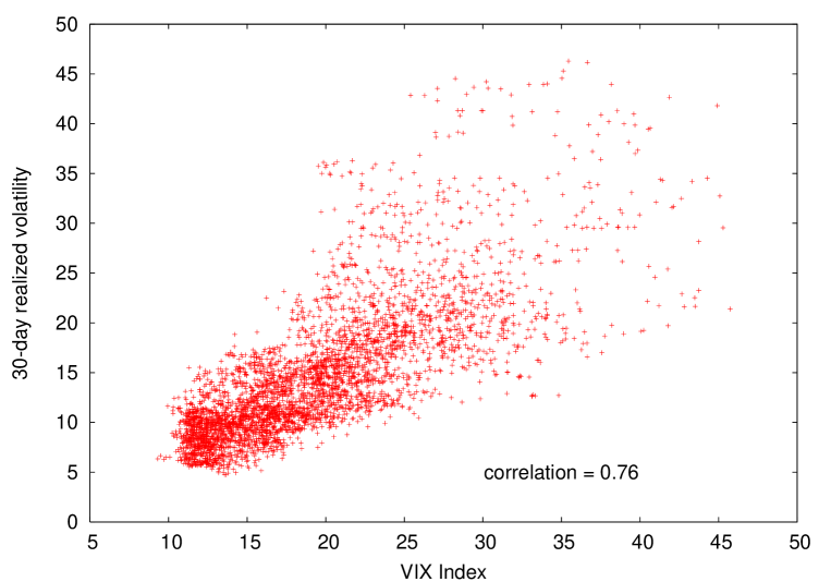
We find a significant correlation between the VIX and the 30-day realized volatility:

\displaystyle{\rm Cor}\left({\rm VIX}_{t},{\rm RVol}_{t,t+30}\right)=0.76.

(3)

Scatter plots of combinations of the VIX, the 30-day realized volatility, and the SPX are shown in Figs. 1, 2, and 3. The correlations between the SPX and both realized and implied volatilities are not significant over long timescale of our sample (16 and a half years).

II.2 Changes in the SPX, the VIX, and realized volatility

In order to examine correlations between changes in the indexes, we make the following definitions:

	$\displaystyle{\rm CSPX}_{t}=\frac{{\rm SPX}_{t}-{\rm SPX}_{t-1}}{{\rm SPX}_{t-1}}$
	$\displaystyle{\rm CVIX}_{t}=\frac{{\rm VIX}_{t}-{\rm VIX}_{t-1}}{{\rm VIX}_{t-1}}.$		(4)

There is a significant negative correlation between changes in the VIX and changes in the SPX:

\displaystyle{\rm Cor}\left({\rm CVIX}_{t},{\rm CSPX}_{t}\right)=-0.66.

(5)

See Fig. 4 for a scatter plot of CVIX_t versus CSPX_t. Note that this negative correlation is interesting, as it implies that there is a non-trivial memory in price dynamics which goes beyond the most naive (i.e., log-normal) models.

In order to examine the correlation between changes in the VIX and changes in the 30-day realized volatility, we must first find a suitable definition for the change in the 30-day realized volatility. To this end, we define:

\displaystyle{\rm CRVol}_{t}=\frac{{\rm RVol}_{t,t+30}-{\rm RVol}_{t-31,t-1}}{{\rm RVol}_{t-31,t-1}}.

(6)

This quantity compares the 30-day realized volatility of the 30-day time period ending at time to time $t-1$ with that of the 30-day time period beginning at time $t$ . It is an appropriate way of measuring the change in the 30-day realized volatility because it compares volatilities of two independent neighboring time periods. However, it remains true that CRVol_t and CRVol_t+1 are not independent. Therefore, in estimating the correlation between the change in the VIX and the change in the 30-day realized volatility, it would not be appropriate to simply compare the two time series CRVol_t and CVIX_t. Instead, we compare the correlation between CRVol_s+30t and CVIX_s+30t for all offsets $s$ with $0<s<30$ . All 21 such time series consist of 196 days (there are 21 trading days for every 30 calendar days). See Fig. 5 for a scatter plot of CRVol_s+30t versus CVIX_s+30t for the case $s=2$ , i.e., the first change in the 30-day realized volatility considered is between the 30 days prior to and the 30 days following 5 Feb 1990. For this choice of offset, the correlation is typical of the values obtained for all values of $s$ , with a value of 0.13.

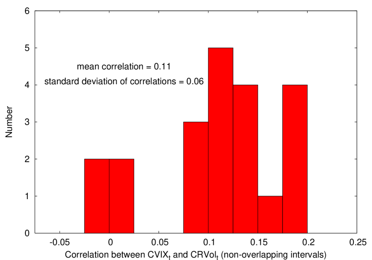
A histogram of the correlations for all possible values of offset $s$ is shown in Fig. 6. Each of the 21 correlations computed is correlating two time series (CVIX_t and CRVol_t) of 196 days each. With a mean correlation of 0.11 and a standard deviation of the correlations of 0.06, it is clear that a change in the VIX does not predict a change in the 30-day realized volatility of the SPX.

III The behavior of implied volatility

In order to try to determine the cause of the negative correlation between changes in the SPX and changes in the VIX, we obtained closing prices for near-the-money SPX put and call options on the days immediately before and the days of the four largest VIX increases and four largest VIX decreases of 2005 and 2006. The data were obtained from Bloomberg.

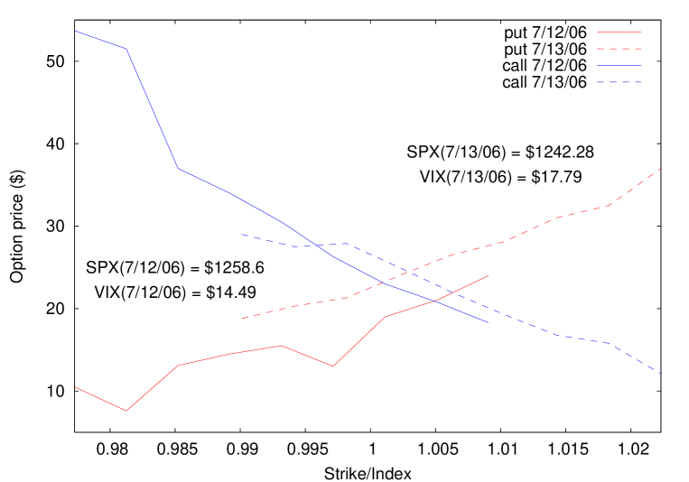
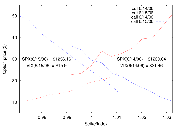
In Figs. 7 and 8 we plot option price versus the ratio of strike price to index level for both puts and calls the day before and the day of one of the largest VIX increases and decreases, respectively, of 2006. As expected, both puts and calls at a given distance from at-the-money become more expensive when VIX increases and less expensive when VIX decreases.

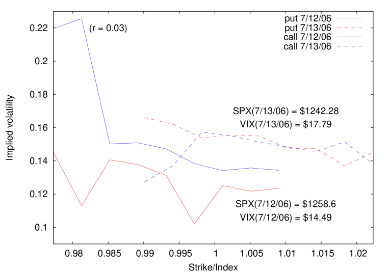
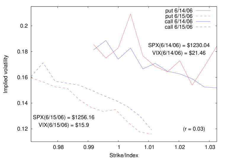
Similarly, the volatility surface is plotted in Figs. 9 and 10. Although we see that, as expected, Black-Scholes implied volatility increases or decreases when the VIX does, it is difficult to comment as to why the VIX is changing, i.e., which particular options are causing the VIX to increase or decrease. Also, we see roughly linear volatility skews, as have been present in many indexes, since the 1987 crash.

Without much more data, we cannot say which options cause the VIX to change. Put gouging, call overwriting or Black’s “leverage effect” may be at work here, but we cannot say with any certainty. It would be interesting to further investigate the volatility surface.

IV Trading realized and implied volatility

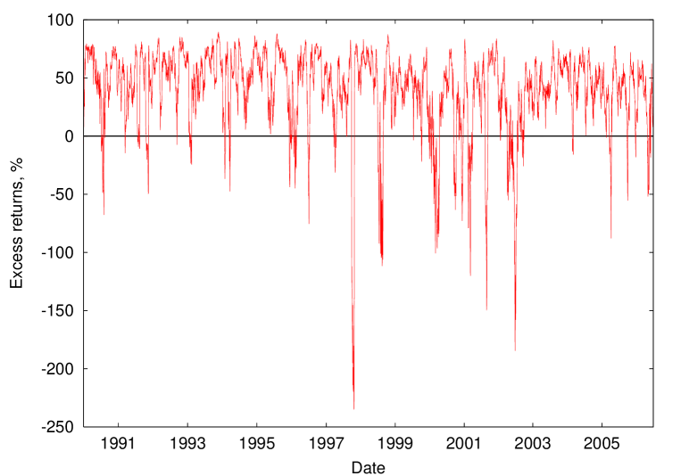
As stated in Sec. I, the VIX has a concrete economic meaning: its square is the variance swap rate up to corrections due to the fact that there are only SPX options at a finite number of strikes, as well as the fact that there are occasional jumps in the underlying (the SPX). In Ref. carr , Carr and Wu use this fact to determine the excess returns that would have been gained from shorting variance swaps on every day of the sample period, where the excess return is defined as:

\displaystyle{\rm ER}_{t,t+30}=100\times\frac{{\rm VIX}_{t}^{2}-{\rm RVol}_{t,t+30}^{2}}{{\rm VIX}_{t}^{2}}.

(7)

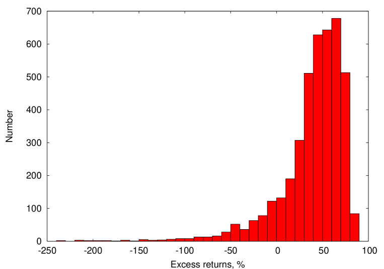
See Figs. 11 and 12 for a time series and a histogram, respectively, of the excess returns.

It is worth emphasizing the fact that the mean excess return gained from continuously shorting variance swaps is large, at nearly 40 percent. Why is this premium so large? In order to answer this question, one must take into account that the distribution of excess returns is heavily skewed; there are a number of occurrences of very large negative excess return. As discussed in Sec. I, parties on the long side of variance swaps are willing to pay a high premium for the insurance provided against periods of high realized volatility (relative to the VIX). Whether they are portfolio managers who are judged against a benchmark, equity funds or others, they are effectively short volatility, and are therefore willing to pay for the insurance that variance swaps provide. Interestingly, Carr and Wu carr argue that the CAPM cannot fully account for the size of the excess return associated with variance swaps. This perhaps indicates an inefficiency or mispricing in this market.

In Sec. II.2 it was shown that there is no correlation between changes in the VIX and changes in the 30-day realized volatility of the SPX. This means that the excess returns gained from shorting 30-day variance swaps would increase if the swaps are shorted only on days when there is a large increase in the VIX as opposed to every day as in Carr and Wu carr . This is true because a change in the VIX does not predict a change in the 30-day realized volatility. Therefore, on average the payoff from shorting the swap will be higher when the VIX has recently increased. The opposite should be true as well: shorting swaps only on days when there is a large decrease in the VIX should lead to a decrease in the excess returns.

Number of days swaps are shorted	$\overline{ER}$	$s_{ER}$	$\overline{ER}/s_{ER}$
4157 (entire sample)	39.45	36.62	1.08
415 (largest VIX increases)	40.43	35.79	1.13
83 (largest VIX increases)	43.20	35.03	1.23
415 (largest VIX decreases)	35.25	40.81	0.86
83 (largest VIX decreases)	31.10	46.53	0.67

Table 1: Average excess return

\overline{ER}

, the standard deviation of the excess returns

s_{ER}

, and the ratio of the two for various trading strategies. Strategies involving the shorting of 30-day variance swaps only on days when there is a large increase in the VIX slightly outperform a strategy in which the swaps are shorted on every day. Shorting only on days when there is a large decrease in the VIX does worse.

Table 1 shows the average excess return $\overline{ER}$ , the standard deviation of the excess returns $s_{ER}$ , and the ratio of the two for various trading strategies. As predicted based on the independence of changes in the VIX relative to changes in the 30-day realized volatility, we see that strategies involving the shorting of 30-day variance swaps only on days when there is a large increase in the VIX slightly outperform a strategy in which the swaps are shorted on every day, while shorting only on days when the VIX experiences a large decrease does worse.

The effect, however, appears to be small. Presumably, this is the case because the average excess return is so large for the simplest trading strategy in which the swaps are shorted every day. Even in the case where one shorts only on the days with the largest one percent of VIX increases, the relative improvement in the average excess return does not appear to be significant. In addition, we considered the possibility of further restricting the trading strategy such that one is only engaged in one swap contract at a time. Again, such a strategy does not do significantly better than the strategy of shorting every day.

V Conclusion

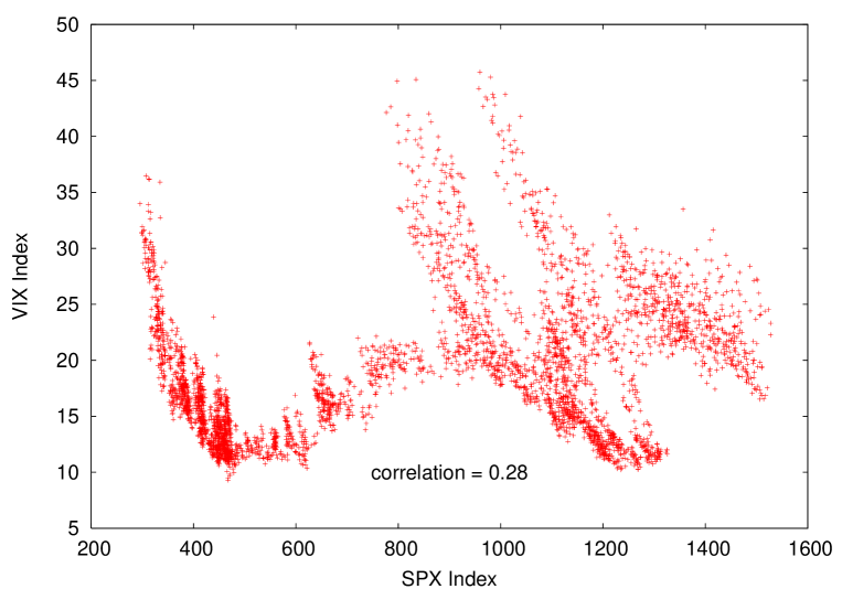
We investigated a number of features of implied and realized volatility of the SPX index. Sec. II examines correlations between the SPX, the VIX, and the 30-day realized volatility of the SPX, as well as between changes in these quantities. We confirmed that the VIX and the 30-day realized volatility are correlated, and that while changes in the SPX are negatively correlated with changes in the VIX, the levels of the two indexes are not correlated over the nearly 16 years of data that we analyzed (although they may be negatively correlated on shorter timescales). Interestingly, as shown in Fig. 6, we found no significant correlation between changes in the VIX and changes in the 30-day realized volatility of the SPX. This means that short term changes in the VIX do not correctly predict the actual realized volatility, and suggests that at least some options are mispriced after large moves in the index.

The details of the negative correlation between changes in the SPX and changes in the VIX were addressed in Sec. III. Without a large dataset of historical options prices, it is difficult to identify the cause of the negative correlation between changes in the SPX and changes in the VIX. To this end, it would be interesting to examine the volatility surface in more detail on days with large market moves.

We returned to the issue of correlation between realized and implied volatility in Sec. IV. We began by reproducing the analysis of Carr and Wu carr regarding the excess return obtained by continuously shorting variance swaps on every trading day of the sample period. We then analyzed whether improved returns could be gained by selectively shorting variance swaps using large changes in the VIX as a signal. In the insurance analogy, this strategy would be similar to an insurance company carefully selecting when to sell insurance policies based on their expectations about the excess returns to be had given a particular trigger criterion (e.g., selling hurricane insurance when demand is high, but the intrinsic probability of a storm has not changed from its historical value). The lack of correlation identified in Sec. II between changes in the VIX and changes in the 30-day realized volatility suggests that this strategy would outperform simply continuously shorting variance swaps. This appears to be the case although statistics are limited. Due to the large premium (excess returns) already associated with variance swaps, we find that the additional advantage is relatively small.

VI Acknowledgements

We thank Myck Schwetz (PIMCO) for useful comments and some help with historical data, and Thomas Gould (CSFB) for additional feedback.

References

(1) Demeterfi, K., E. Derman, M. Kamal, and J. Zou. “More Than You Ever Wanted to Know About Volatility Swaps.” Quantitative Strategies Research Notes, March 1999, Goldman, Sachs & Co.
(2) Carr, P., and L. Wu. “A Tale of Two Indices.” Working paper, New York University, 2006.
(3) Black, F., and M. Scholes. “The Pricing of Options and Corporate Liabilities.” Journal of Political Economy, 81 (1973), pp. 637-654.
(4) Black, F. “Studies of Stock Price Volatility Changes.” In Proceedings of the 1976 American Statistical Association, Business and Economical Statistics Section. Alexandria, VA: American Statistical Association, 1976, pp. 177-181.