Is it possible to observe experimentally a metal-insulator transition in ultra cold atoms?

Abstract

It has been recently reported ant9 that kicked rotators with certain non-analytic potentials avoid dynamical localization and undergo a metal-insulator transition. We show that typical properties of this transition are still present as the non-analyticity is progressively smoothed out provided that the smoothing is less than a certain limiting value. We have identified a smoothing dependent time scale such that full dynamical localization is absent and the quantum momentum distribution develops power-law tails with anomalous decay exponents as in the case of a conductor at the metal-insulator transition. We discuss under what conditions these findings may be verified experimentally by using ultra cold atoms techniques. It is found that ultra-cold atoms can indeed be utilized for the experimental investigation of the metal-insulator transition.

The study of a quantum particle in a random potential anderson is one of the cornerstones of modern condensed matter physics. In its simplest form, namely, a free spin-less particle in a short-range disordered potential with no interactions at zero temperature, the combination of the one parameter scaling theory one , the supersymmetry method efetov and numerical simulations schreiber has led to the following picture: In two and lower dimensions destructive interference caused by backscattering produces exponential localization of the eigenstates in real space for any amount of disorder. As a consequence, quantum transport is suppressed, the spectrum is uncorrelated (Poisson) and the system becomes an insulator. In more than two dimensions there exists a metal insulator transition (usually referred to as Anderson transition (AT))for a critical amount of disorder. By critical disorder we mean a disorder such that, if increased, all the eigenstates become exponentially localized. For a disorder strength below the critical one, the system has a mobility edge at a certain energy which separates localized from delocalized states. Its position moves away from the band center as the disorder is decreased. Delocalized eigenstates, typical of a metal, are extended through the sample and the level statistics agree with the random matrix prediction for the appropriate symmetry. In three and higher dimensions the AT takes place in a region of strong disorder only accessible to numerical schreiber ; multi simulations. Typical features of the AT include:

1. The spectrum of the Hamiltonian is scale invariant sko , namely, any spectral correlator utilized to describe the spectral properties of the disordered Hamiltonian does not depend on the system size. The spectral correlations at the AT, usually referred to as critical statistics sko ; kravtsov97 , are intermediate between that of a metal and that of an insulator.

2. Anomalous scaling of the eigenfunction moments, ${\cal P}_{q}=\int d^{d}r|\psi({\bf r})|^{2q}\propto L^{-D_{q}(q-1)}$ with respect to the sample size $L$, where $D_{q}$ is a set of exponents describing the AT. Eigenfunctions with such a nontrivial (multi) scaling are usually dubbed multifractals multi (for a review see cuevas ).

3. Quantum diffusion is anomalous huck at the AT. In the metallic limit, up to small weak localization corrections, the density of probability is Gaussian-like and the dynamics is well described by a Brownian motion. However, as disorder increases, localization effects become important and quantum diffusion slows down. The density of probability develops power-law tails with a decay exponent depending on the spectrum of multifractal dimensions huck .

Unfortunately the experimental verification of the AT is a challenging task. In the context of electronic systems is extremely hard to disentangle effects caused by short decoherence times, electron-electron interactions and phonon-electron interactions from destructive quantum interference and symmetry, supposed to be the main ingredients driving the AT.

In recent years ultracold atoms in optical lattices raizen has been utilized to model certain solid state physics systems. Generically, in these experiments a very dilute almost free gas of atoms (Cs and Rb) is cooled up to temperatures of the order of tens $\mu K$ and then interacts with an optical lattice. In its simplest form, the optical lattice consists of two laser beams prepared in such a way that the resulting interference pattern is a stationary plane wave in space. The laser frequency is tuned close to a resonance of the atomic system in order to enhance the atom-laser coupling but not too close to avoid spontaneous emission. In this limit the system laser-atom can be considered as a point particle in a sine potential, namely, the quantum pendulum. Additionally if the laser is turned on only in a series of short periodic pulses the resulting system is very well approximated by the so called quantum kicked rotor (see reviz for a review) extensively studied in the context of quantum chaos,

$${\cal H}=p^{2}/2+k\cos(q)\sum_{n}\delta(t-Tn).$$ (1)

The classical motion of this system is diffusive in momentum space. For short time scales, quantum and classical motion agrees. However quantum diffusion is eventually suppressed due to interference effects and eigenstates are exponentially localized in momentum space. This counterintuitive feature, usually referred to as dynamical localization dyn , was fully understood fishman after mapping the kicked rotator problem onto an short range 1D disordered system where localization is well established. The first direct experimental realization of the kicked rotor was reported in Ref. raizen . As was expected, the output of the experiment (the distribution of the atom momentum and the energy diffusion as a function of time) fully agrees with the theoretical prediction of dynamical localization fishman . Finally we remark that, after the pioneering work of Ref.raizen , many other aspects of the physics of a quantum kicked rotor as the effect of noise and dissipation have also been investigated otherexp by using similar experimental settings.

The above results do not depend on the exact details of the potential but only on its ability to produce classical chaotic motion. The situation is different if the potential is not smooth. Recently ant9 it has been reported that a kicked rotor could avoid full dynamical localization if the smooth sinusoidal optical potential is replaced with a generic potential with a logarithmic or step like singularity. It was found that, for these potentials, the kicked particle has striking similarities with a free particle in a disordered potential at the AT. Thus level statistics are given by critical statistics, eigenfunctions are multifractal and quantum diffusion becomes anomalous.

A natural question to ask is whether this non-analytical kicked rotor can be realized in experiments. If so, this would be an ideal setting to test the physics of the AT. Obviously, in experiments the singularity can only be approximated. For instance, an optical lattice potential with an approximate step-like singularity can be produced gar either by a holographic mask mask with precision $\sigma$ or by adding a limited number of Fourier components. In both cases the potential is smooth on sufficiently small scales $\sim\sigma$. That means that for momenta $p_{d}\gg\hbar/\sigma$ and times $t_{d}$ sufficiently long, the microscopic smoothness of the potential is at work and standard dynamical localization should be observed. On the other hand, for momenta $p_{c}$ and times $t_{c}$ sufficiently short, classical and quantum results should coincide. In between these two scales typical properties of the AT are observed. The aim of this paper is twofold on the one hand we seek to determine in what window of $\sigma$ the AT is observed. On the other hand we examine whether this range is already experimentally accessible by using ultra cold atoms in optical lattices.

The organization of the paper is as follows: In the next section we introduce a kicked rotor with two different smoothed out versions of a step potential. Then we evaluate the rate of energy diffusion and the full momentum distribution. Finally we establish the minimum smoothing required to observe the AT and whether an experimental verification is realistic with the current, state of the art, ultra cold atom techniques.

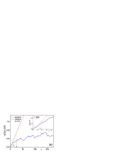
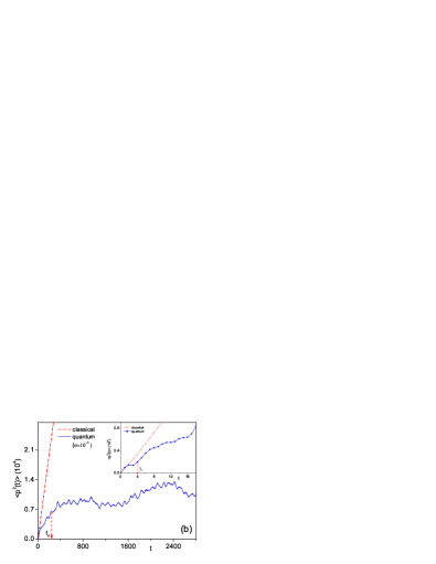
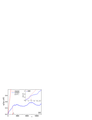
Figure 1: (Color online)Comparison of quantum and classical energy diffusion versus time for different smoothings: $\sigma=5\times 10^{-2}$ (a), $\sigma=10^{-2}$ (b) and $\sigma=10^{-3}$ (c). Quantum initial conditions, $|\psi(0)\rangle=|0\rangle$, were chosen to mimic its classical counterpart. For $t<t_{c}$ quantum and classical diffusion rates are similar. For $t_{d}\approx 2/\sigma$ the quantum energy diffusion gets saturated due to destructive interference. In between these two scales the system behaves as a disordered conductor at the AT.

I The model and observables

We investigate a kicked rotor in $1+1$D with a smoothed step-like potential,

$${\cal H}=\frac{p^{2}}{2}+V_{1,2}(q)\sum_{n}\delta(t-nT)$$ (2)

with $q\in[-\pi,\pi)$. We consider the following two potentials,

$$V_{1}(q)=Si\left((\frac{\pi}{2}+q)/\sigma\right)+Si\left((\frac{\pi}{2}-q)/\sigma\right)$$ (3)

where $Si(q)=\int_{0}^{q}\frac{\sin(t)}{t}dt$ is the sine integral function, and

$$V_{2}(q)=\sum_{m=0}^{M}f(m)\cos(mq)$$ (4)

where $f(m)$ is the discrete Fourier transform of the bare step like potential $V(q)=\pi$ for $|q|<\pi/2$ and zero otherwise. In both cases for $\sigma\rightarrow 0$ ($\sigma\equiv 1/M$ in the latter case) we recover the bare step-like potential investigated in ant9 . Obviously there are infinitely many ways to smooth a singularity, we have chosen the above two due to similarities with the experimental situation. Thus $V_{1}(q)$ represents an optical lattice with square-wave intensity profile as produced by an array of fine slits or a holographic mask mask . The other potential $V_{2}(q)$ produces an approximated step-like shape by adding a limited number of Fourier components. We remark that results for $V_{1}(q)$ and $V_{2}(q)$ are hardly distinguishable, both are smooth and oscillatory on scales of the order of $\sigma$. Numerically it is a little easier to simulate $V_{1}(q)$ so we will stick to it for the numerical calculations.

We analyze both the classical and the quantum motion of the above Hamiltonian. The classical evolution over a period $T$ is dictated by the map: $p_{n+1}=p_{n}-\frac{\partial V(q_{n})}{\partial q_{n}}$, $q_{n+1}=q_{n}+Tp_{n+1}$ (mod$~{}2\pi$). By smoothing the step potential the classical force has a well defined classical limit for any finite $\sigma$.

The quantum dynamics is governed by the quantum evolution operator $\cal U$ over a period $T$. Thus, after a period $T$, an initial state $\psi_{0}$ evolves to $\psi(T)={\cal U}\psi_{0}=e^{\frac{-i{\hat{p}}^{2}T}{2{\bar{h}}}}e^{-\frac{iV(\hat{q})}{\bar{h}}}\psi_{0}$ where $\hat{p}$ and $\hat{q}$ stands for the usual momentum and position operator. Our aim is to evolve a given initial state to a certain time $nT$. This is equivalent to solving the eigenvalue problem ${\cal U}\Psi_{n}=e^{-i\kappa_{n}/\hbar}\Psi_{n}$ where $\Psi_{n}$ is an eigenstate of $\cal U$ with quasi-eigenvalue $\kappa_{n}$. In order to proceed we can express the evolution operator $\langle m|{\cal U}|n\rangle=U_{nm}$ in the basis of momentum eigenstates $\{|n\rangle=\frac{e^{in\theta}}{\sqrt{2\pi}}\}$ with $n=0,\ldots N\rightarrow\infty$,

$$U_{mn}=\frac{e^{-i\frac{T\hbar}{4}(m^{2}+n^{2})}}{2\pi}\int_{-\pi}^{\pi}dqe^{iq(m-n)-iV(q)/\hbar}$$ (5)

We remark that in this representation, referred to as ‘cylinder representation’, the resulting matrix $U_{nm}$ is unitary exclusively in the $N\rightarrow\infty$ limit. This is certainly a disadvantage since besides typical finite size effects one has also to face truncation effects, namely, the integral of the density of probability is not exactly the unity and eigenvalues are not pure phases ($e^{-i\theta_{n}}$) as expected in a Unitary matrix. Moreover the diagonalization of a generic non Unitary matrix is numerically much more demanding.

These difficulties can be circumvented by changing representations in each quantum iteration step, a technique extensively adopted in quantum kicked rotator studies. First, we express a given state $\psi$ in position representation, so that it is straightforward to get $\psi^{\prime}=e^{-\frac{iV(\hat{q})}{\bar{h}}}\psi$, the state just after the kick. Next, we express $\psi^{\prime}$ in the angular momentum representation by using the fast Fourier transformation (FFT) algorithm to facilitate the calculation of $e^{\frac{-i{\hat{p}}^{2}T}{2{\bar{h}}}}\psi^{\prime}$. Since no matrix diagonalization is involved in this scheme, the computation is quite fast and the effective dimension of the state vectors is as large as $10^{8}$. As a result the truncation effects mentioned above can be safely neglected. We recall that this method allows to resolve the potential with a precision of $10^{-8}$, four order less than the minimum $\sigma(10^{-4})$ investigated. Such degree of precision is a necessary requirement to determine the effect of a small $\sigma$ in the quantum transport properties of the model studied.

Analytical results for the above model can in principle be obtained by mapping Eq.(2) onto an 1D Anderson model. This method was introduced in fishman for the case of a kicked rotor with a smooth potential. We do not repeat here the details of the calculation but just state how the 1D Anderson model is modified by the non-analytical potential. It turns out that the classical non-analyticity induces long-range disorder in the associated 1D Anderson model. If the kick strength is sufficiently large the diagonal part of the Anderson model is pseudo-random and the off-diagonal one decays as $U_{r}\sim 1/r$ with $r$ the distance from the diagonal. This Anderson model is similar to the one studied in multi which is solved by using the supersymmetry method. In general, according to Ref.multi , a $1/r$ decay in 1D is a signature of an AT. For the potential $V_{1,2}$ above, it is straightforward to show that $U_{r}\sim 1/r$ for $r\ll 1/\sigma$ and $U_{r}\sim e^{-\sigma r}$ for $r>1/\sigma$. Consequently we expect to observe AT like behavior for small momentum and then eventually recover the results of the sinusoidal potential, namely, exponential localization in momentum space. For further details of the analytical approach we refer to ant9 .

We are mainly interested in observables related to transport properties as the density of probability and the rate of diffusion.

The density of probability (both classical $P(p,t)$ and quantum $P_{q}(p,t)$) of finding a particle with momentum $p$ after a time $t$ for a given initial state $|\psi(0)\rangle=|0\rangle$. $P_{q}(p,t)\equiv P_{q}(k,t)=|\langle k|\phi(t)\rangle|^{2}$ with $p=k\hbar$. In all calculations we set $\hbar=1$. The classical $P(p,t)$ is obtained by evolving the classical equation of motion for $2\times 10^{7}$ different initial conditions with zero momentum $p=0$ and uniformly distributed position along the interval $(-\pi,\pi)$. We would like to emphasize our results do not depend on the initial conditions. For instance, we have checked that similar results are obtained if the initial conditions of Ref.rei2 are considered.

We also examine the second moment of the probability distribution, namely, the energy diffusion $\langle p^{2}(t)\rangle=\int_{0}^{\infty}dpp^{2}P(p,t)$ as a function of time.

We recall our aim is to find out whether the transport properties are compatibles with those of a disordered conductor at the AT and how they are affected by the short distance differentiability of the potential. For the sake of completeness let us briefly summarize the predictions for both a kicked particle in a smooth potential and a disordered conductor at the AT.

For a kicked rotator with a smooth potential, it is well established that initially (up to a certain time $t_{c}$) both classical and quantum probabilities are Gaussian like and the diffusion in momentum is normal, namely, a standard Brownian motion. For longer times the classical density of probability is still that of a normal diffusion process. However $P_{q}(p,t)$ become exponentially localized and energy diffusion stops $\langle p^{2}(t)\rangle\sim cons$. These are typical signatures of dynamical localization.

At the AT, up to a certain $t_{c}$, agreement is also expected between the classical and quantum predictions. In the case of a disordered conductor the classical dynamics is obviously well described by a Brownian motion. However, for $t>t_{c}$, the diffusion becomes anomalous, the quantum density of probability develop power-law tails in space (localization in a disordered conductor occurs in real space) and time with exponents related to the multifractal dimensions of the eigenstates huck . The rate of diffusion is in some cases still similar to the one corresponding to normal diffusion $\langle p^{2}(t)\rangle=D_{quan}t$ though the quantum diffusion constant $D_{quan}$ is typically lower. This suggests that, at the AT, destructive interference is still at work but it is not sufficient to fully localize the particle. In our case we also expect agreement between classical and quantum results up to a certain time $t_{c}(\sigma)$. Additionally, since the potential is differentiable for distances smaller than the smoothing $\sigma$, we expect that there exists a $t_{d}(\sigma)$ such that for $t\gg t_{d}$ standard dynamical localization becomes dominant.

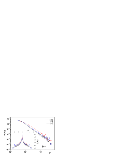
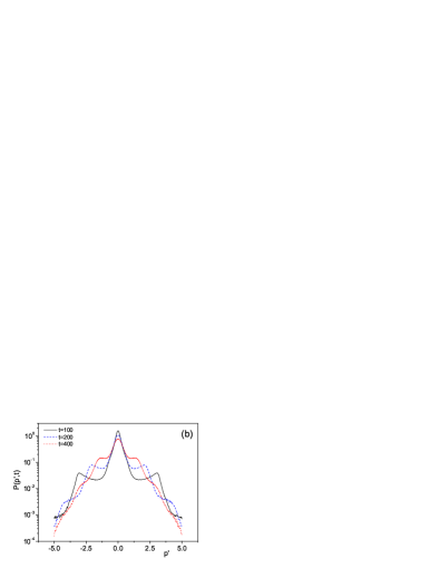
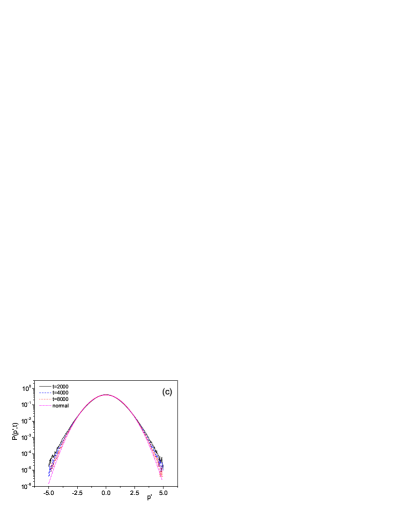
Figure 2: (Color online) Classical density of probability distribution $P(p^{\prime},t)$ for $\sigma=10^{-3}$ and $p^{\prime}=p/\sqrt{2Dt}$. (a) Region of anomalous diffusion, $t<10$, (b) Crossover from anomalous to normal diffusion $10<t<t_{d}\approx 2/\sigma$ and (c) Normal diffusion $t>t_{d}$. The results were obtained after averaging over $2\times 10^{7}$ initial conditions.

Typical features of the AT transition are thus observed in our model only if $t_{c}\ll t_{d}$. It is unclear for what range of $\sigma$, $t_{d}\gg t_{c}$ and whether these values of $\sigma$ can be reached experimentally. We answer these questions in the next section.

II Results

For the sake of clearness we first enunciate our main conclusions:

1. For $\sigma\leq 0.05$ we have observed typical signatures of an AT in a broad region of times $t_{c}\gg t\gg t_{d}$.

2. The quantum-classical breaking time $t_{c}$ decreases weakly with $\sigma$. In the range of $\sigma$ investigated it never goes beyond a few kicks. By contrast, the time scale signaling the beginning of full dynamical localization, due to the differentiability of the potential, increases as $\sigma$ decreases, $t_{d}\approx 2/\sigma$.

3. We argue that the above range of parameters is accessible to experimental verification. By using holographic mask techniques one can reach up to $\sigma\sim 0.01$ gar . On the other hand coherence in ultra cold atoms is maintained well beyond $1000$ kicks. Consequently the AT can be investigated by using ultracold atoms in optical lattices.

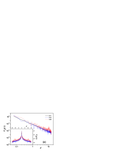
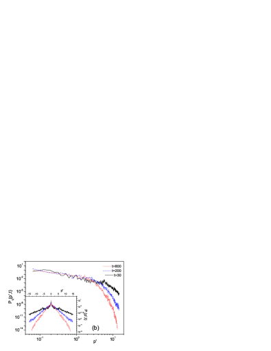
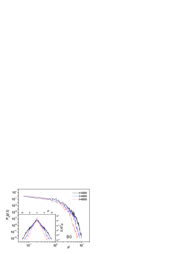
Figure 3: (Color online) Quantum density of probability distribution $P_{q}(p^{\prime},t)$, $p^{\prime}=p/\sqrt{2Dt}$ and $\sigma=10^{-3}$ for three different regions: (a) $t<t_{c}\leq 10$, agreement between classical and quantum results, (b) $t_{c}<t<t_{d}$, typical properties of an AT are observed, and (c) $t>t_{d}$, standard dynamical localization for $|p|>\sqrt{2Dt_{d}}$. In the insets we present the same results in a linear-log scale. $P_{q}(p^{\prime},t)\sim 1/p^{2}$ for $t<t_{c}$ and $|p|^{\prime}<1$, and $P_{q}(p^{\prime},t)\sim 1/p^{\alpha}$ with $\alpha=1.1\pm 0.2$ for $t>t_{c}$. As initial condition we used $|\psi(0)\rangle=|0\rangle$.

We have computed (see details in previous section) the quantum and classical density of probability for the Hamiltonian Eq. 2 with potentials given by Eq.3 and a variety of smoothings $\sigma\in[0.1,10^{-4}]$.

Our first task is to determine $t_{c}$ and $t_{d}$ as a function of $\sigma$. These time scales can in principle be calculated by using different observables. Qualitatively all observables should provide the same physical picture. However the numerical value of $t_{c}$ and $t_{d}$ may depend on the observable considered. For the sake of simplicity we estimate these time scales by looking at the the rate of energy diffusion $\langle p^{2}(t)\rangle$.

II.1 Energy diffusion

As was mentioned previously we used as initial conditions $p=0$ and random positions. Obviously only initial conditions in the narrow region $[-\pi+\sigma,\pi-\sigma]$ get a sizable kick. Thus even after several kicks there is a high probability that the system stays in the region $p=0$. In order to show that our results are not sensitive to initial conditions and stable under perturbations we have added a weak noise $V(q)=k\sin(q)$ with $k=1$. We have checked our results do not depend on $k$ provided $k\ll 1/\sigma$. Obviously for $k\sim 1/\sigma$ the effect of the pseudo-singularity is obscured by the noise strength. In the classical case (see Fig.1 ) $\langle p^{2}(t)\rangle$ increases linearly with time. The dependence of the diffusion coefficient on $\sigma$ is well approximated by $0.5/\sigma$. This is consistent with the the analytical prediction resulting from the random phase approximation lich . In the quantum case (see Fig.1 ) we distinguish three different regions. In a first stage ($t<t_{c}\leq 10$) the quantum averaged energy moves around its classical counterpart. $t_{c}$ depends weekly on $\sigma$, it decreases as $\sigma$ does. For longer times $t_{c}<t<t_{d}$, the diffusion is still linear, $\langle p^{2}(t)\rangle\approx D_{quan}t$, with $D_{quan}\sim 0.2/\sigma$. Although it has the same dependence on $\sigma$, it is smaller than in the classical case. This suggests that quantum interference effects slow down the classical diffusion. A similar feature has been found in a disordered conductor at the AT huck . This stage lasts up to $t_{d}\approx 2/\sigma$. For longer times standard dynamical localization due to the differentiability of the potential takes over and diffusion stops.

We recall that linear energy diffusion is only a necessary condition for normal diffusion. In general the information obtained from the knowledge of a few moments of the distribution is not sufficient to fully characterize the classical motion. Thus the second moment may be $\langle p^{2}(t)\rangle\sim t$ but this by no means assures that the density of probability is Gaussian-like klafter as for normal diffusion. We show below that this is the case in our model.

II.2 Density of probability

In the classical case we distinguish two different regimes separated by a broad crossover region (see density of probability in Fig.2): First, for short time scales (a few kicks) and $|p|<c(\sigma)\sqrt{2Dt}$ the diffusion is anomalous. $P(p,t)\sim p^{-\alpha}$ with $\alpha\sim 2$ and $c(\sigma)\approx 1$ slightly increases as $\sigma$ is decreased. For such a short time scale the classical system does not feel the differentiability of the potential.

For longer times but $t<t_{d}$, we observe a gradual crossover from anomalous to normal diffusion. For small momentum the density is still non Gaussian as the effect of the pseudo non differentiability is still important. As time approaches $t_{d}$, the central (small momentum) non-Gaussian region becomes smaller and smaller. Meanwhile, the outskirts bend down and a Gaussian-like behavior typical of normal diffusion is observed. Finally, for $t>t_{d}$, $P(p,t)$ is well approximated by a Gaussian distribution. These regions have been observed for all $\sigma$ of interest.

In the quantum case three regimes are distinguished (see Fig. 3):

1. $t<t_{c}$ and $|p|<c(\sigma)\sqrt{2Dt}$ with $D\approx 0.5/\sigma$ ($c(\sigma)$ increases slightly as $\sigma$ decreases). The classical and the quantum probability agree in this region. The scale $t_{c}$ depends weakly on $\sigma$; it decreases as $\sigma$ does. We recall that our system has not a well defined classical-quantum correspondence in the limit $\sigma\rightarrow 0$. In both cases the diffusion is anomalous $P(p,t)=P_{q}(p,t)\sim 1/p^{2}$. We remark $P_{q}(p,t)$ is calculated by summing the probability of falling in a bin of width $\Delta p^{\prime}=0.03$ (so does for classical $P(p,t)$), hence it is in fact a coarse-grained result where part of quantum fluctuations have been suppressed.

2. For $|p|<c(\sigma)\sqrt{2Dt}$ but $t_{d}>t>t_{c}$. The quantum probability $P_{q}(p,t)\sim 1/p^{\alpha}$ develop an power-law tail with an exponent $\alpha<2$ (see Fig. 3) typical of anomalous diffusion. The exponent $\alpha$ does not depend on $\sigma$, in all cases we have found $\alpha\sim 1.1\pm 0.2$. This is a clear signature of an AT. We remark that, in agreement with previous results from the energy diffusion, the quantum decay is slower than the classical one. Quantum interference slows down the motion but it is not enough to fully localize the particle.

3. For $|p|>c(\sigma)\sqrt{2Dt}$ and $t>t_{d}$, $P_{q}(p,t)$ decays exponentially. This is an indication of full dynamical localization due to the differentiability of the potential.

$\sigma$	$t_{c}$	$t_{d}$
$1\times 10^{-1}$	$~{}~{}7\pm 4$	$~{}~{}~{}11\pm 3$
$5\times 10^{-2}$	$~{}~{}7\pm 4$	$~{}~{}~{}35\pm 10$
$2\times 10^{-2}$	$~{}~{}7\pm 4$	$~{}~{}~{}50\pm 25$
$1\times 10^{-2}$	$~{}~{}7\pm 4$	$~{}~{}~{}250\pm 50$
$5\times 10^{-3}$	$~{}~{}8\pm 4$	$~{}~{}~{}410\pm 100$
$2\times 10^{-3}$	$~{}~{}8\pm 4$	$~{}~{}~{}1300\pm 250$
$1\times 10^{-3}$	$~{}~{}8\pm 4$	$~{}~{}~{}2000\pm 400$
$5\times 10^{-4}$	$~{}~{}8\pm 4$	$~{}~{}~{}4800\pm 1200$

Table 1: Time scales $t_{c}$ and $t_{d}$ for various values of $\sigma$

From the above we can affirm that in order to observe typical features of an AT in the transport properties of our system, $t_{c}$ and $t_{d}$ must be well separated, namely, $t_{d}\gg t\gg t_{c}$. As is shown in Fig. 3 and Table I, this occurs provided that $\sigma\leq 0.05$. Thus for an experimental verification of the AT in cold atoms one has to manage to produce a bare step-potential up to corrections of order $\sigma\leq 0.05$

II.3 Experimental verification

A natural question to ask is what is the minimum values of $\sigma$ that it can be reached in experiments. Specifically, we wish to determine, for instance, the maximum number of terms in $V_{1}(q)$ that can be included experimentally. In principle gar it is an challenging experimental task to realize optical potentials with high slopes involving higher optical harmonics of the laser beam. The problem is that, for instance for Cs, the fourth harmonic is already in the vacuum UV, and difficult to produce. Additionally higher order harmonics are not resonant with the atom and need a much stronger intensity. Thus it seems extremely hard to go beyond the first few harmonics. Another option could be to use a kicked rotor with a smooth potential and three incommensurate frequencies. According to the results of shepe , this model can be mapped it onto a 3D Anderson model which is supposed to undergo an AT for a specific value of the coupling constant. However in more than one dimension there is no clear evidence that this mapping is really accurate. For instance, the critical exponents at the AT are very different from the one found in the kicked rotor with three incommensurate frequencies she1 .

A more promising alternative is to use a holographic mask to give a square-wave intensity profile mask . This technique combined with the recent introduction of spatial light modulators permit the production of a very broad range of intensity pattern which act as a effective spatial potential for atoms. Unlike the previous method the sharpness of the edges would be limited by diffraction effects of the order of the wavelength gar . With the current techniques the potential of Eq.3 could be produced in a window $\sigma\geq 10^{-2}$. On the other hand quantum coherence in cold atoms is lost after a few thousands kicks. The experimental bounds are thus within (see above) the theoretical limits and, as a consequence, the AT can be studied by using ultra cold atoms in optical lattices.

In conclusion, we have explicitly shown that kick rotors with a singular but slightly smoothed potential still have similar transport properties that those of a disordered conductor at the AT provided that the degree of smoothing is weak enough. The utilization of ultra cold atoms in optical lattices offers the opportunity to investigate Anderson localization in general and the AT in particular in a setting free from many of the inconveniences that have plagued other experimental studies of the AT in the context of condensed matter physics.

- (1) P.W. Anderson, Phys. Rev. 109, 1492 (1958).
- (2) E. Abrahams et al., Phys. Rev. Lett. 42, 673 (1979).
- (3) K.B. Efetov, Adv. Phys. 32 53 (1983).
- (4) M. Schreiber and H. Grussbach, Phys. Rev. Lett. 67, 607 (1991);A. McKinnon and B. Kramer, Phys. Rev. Lett. 47, (1981) 1546. Phys. Rev. Lett. 81, 268 (1998); Nucl. Phys. B525, 738 (1998)
- (5) H. Aoki, J. Phys. C 16, L205 (1983); A.D. Mirlin et al., Phys. Rev. E 54 3221 (1996); F. Evers and A.D. Mirlin, Phys. Rev. Lett. 84, 3690 (2000); E. Cuevas et al., Phys. Rev. Lett. 88, 016401 (2002).
- (6) B.I. Shklovskii, B. Shapiro, B.R. Sears, P. Lambrianides and H.B. Shore, Phys. Rev. B 47, (1993) 11487.
- (7) V.E. Kravtsov and K.A. Muttalib, Phys. Rev. Lett. 79, 1913 (1997); S. M. Nishigaki, Phys. Rev. E 59, (1999) 2853.
- (8) M. Janssen, Int. J. Mod. Phys. B 8, 943 (1994); B. Huckestein, Rev. Mod. Phys. 67, 357 (1995).
- (9) B. Huckestein and R. Klesse, Phys. Rev. B 59, 9714 (1999).
- (10) F. L. Moore, J. C. Robinson, C. F. Bharucha, Bala Sundaram and M. G. Raizen Phys. Rev. Lett. 75, 4598 (1995).
- (11) F.M. Izrailev. Phys. Rep. 196, 299 (1990).
- (12) G. Casati, B. V. Chirikov, F. M. Izrailev and J. Ford, in Stochastic Behavior in Classical and Quantum Hamiltonian Systems, edited by G. Casati and J. Ford, Lecture Noted in Physics Vol. 93 (Springer, Berlin, 1979); B. V. Chirikov, F. M. Izrailev and D. L. Shepelyansky, Sov. Sci. Rev. 2C, 209 (1981).
- (13) S. Fishman, D. R. Grempel, and R. E. Prange, Phys. Rev. Lett. 49, 509 (1982).
- (14) H. Ammann, R. Gray, I. Shvarchuck and N. Christensen Phys. Rev. Lett. 80, 4111 (1998);B. G. Klappauf, W. H. Oskay, D. A. Steck, M. G. Raizen, Phys. Rev. Lett. 81, 4044 (1998);M. B. d’Arcy, R. M. Godun, M. K. Oberthaler, D. Cassettari, G. S. Summy Phys. Rev. Lett. 87, 074102 (2001);J. Gong, H. J. Wörner, P. Brumer, Phys. Rev. E 68, 056202 (2003);H. Lignier, J. Chabé, D. Delande, J. C. Garreau, and P. Szriftgiser Phys. Rev. Lett. 95, 234101 (2005).
- (15) A.M. Garcia-Garcia, J. Wang, Phys. Rev. Lett. 94, 244102 (2005); Phys. Rev. E 73, 036210 (2006);A.M. Garcia-Garcia, Phys. Rev. E 72, 066210 (2005); A. M. Garcia-Garcia and J.J.M. Verbaarschot, Phys. Rev. E 67, 046104 (2003).
- (16) C. F. Bharucha, J. C. Robinson, F. L. Moore, Bala Sundaram, Qian Niu, and M. G. Raizen, Phys. Rev. E 60, 3881 (1999).
- (17) We thank J. F. Garreau and D. A. Steck for teaching us about experimental limitations in the modelling of optical lattice potentials.
- (18) M, Mutzel, S. Tandler, D. Haubrich, et al., Phys. Rev. Lett. 88, 083601 (2002).
- (19) A.J. Lichtenberg, and M.A. Lieberman, Regular and Chaotic Dynamics, 2ed. (Springer-Verlag, New York, 1992).
- (20) J. Klafter and G. Zumofen, Phys. Rev. E 49, 4873 (1994).
- (21) G Casati, I. Guarneri, D.L. Shepelyansky, Phys. Rev. Lett. 62, 345, (1989).
- (22) F. Borgonovi, D.L. Shepelyansky, Physica D109, 24 (1997).