A generic model for lipid monolayers, bilayers, and membranes

Abstract

We describe a simple coarse-grained model which is suited to study lipid layers and their phase transitions. Lipids are modeled by short semiflexible chains of beads with a solvophilic head and a solvophobic tail component. They are forced to self-assemble into bilayers by a computationally cheap ‘phantom solvent’ environment. The model reproduces the most important phases and phase transitions of monolayers and bilayers. Technical issues such as Monte Carlo parallelization schemes are briefly discussed.

, , , ,

1 Introduction

Lipid bilayers are the main components of biological membranes and omnipresent in all living matter gennis . At high temperatures bilayers assume the so-called ‘liquid’ state ($L_{\alpha}$), where lipids are highly mobile and have many chain defects. In nature, this state is the most frequent. If one decreases the temperature, pure one-component lipid bilayers undergo a prominent phase transition, the ‘main’ transition, which is characterized by dropping lipid mobility, dropping number of chain defects, and dropping area per lipid. The structure of the low temperature ‘gel’ phase depends on the bulkiness and interactions of the head groups. For small head groups, the chains are oriented normal to the bilayer ($L_{\beta}$ phase), for larger head groups, they are tilted ($L_{\beta^{\prime}}$). In the latter case, the main transition occurs in two steps, and an undulated intermediate phase emerges, the ‘ripple’ phase $P_{\beta^{\prime}}$. If head groups are large and weakly interacting, such as ether-linked phosphatidylcholines, the system assumes a phase $L_{\beta}^{\mbox{\tiny int}}$ where both opposing lipid layers are fully interdigitated koynova .

In this paper, we present a lipid model which is suited for studying lipid bilayers. We will first apply it to lipid monolayers (Sec. 2) and show that it reproduces the generic features of fatty acid monolayers. Then we introduce an environment model which forces the model lipids to self-assemble into bilayers, and discuss the resulting bilayer phases (Sec. 3). Selected technical issues regarding the Monte Carlo implementation are discussed in the Appendix.

2 Lipids and Monolayers

The lipids are represented by chains of $n-1$ ‘tail’ beads with diameter $\sigma_{t}$, attached to one ‘head’ bead with diameter $\sigma_{h}$. Beads that are not direct neighbors along their chain interact with a truncated and shifted Lennard-Jones potential,

$$V_{LJ}(r)=\epsilon\big{[}\>(\frac{\sigma}{r})^{12}-2(\frac{\sigma}{r})^{6}+v_{c}\>\big{]}\quad\mbox{for}\>r<R_{0},$$ (1)

$V_{LJ}(r)=0$ otherwise, with $v_{c}$ chosen such that $V_{LJ}(r)$ is continuous at $r=R_{c}$. The parameter $\sigma$ is the arithmetic mean of the diameters of the two interacting beads. Head-head interactions and head-tail interactions are purely repulsive, which is ensured by choosing $R_{0}=\sigma$. Tail-tail interactions have an attractive part, $R_{0}=2\sigma$.

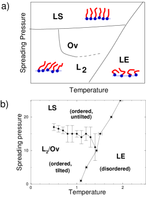
Figure 1: Monolayer phase diagrams. (a) Generic phase diagram for fatty acid monolayers (after Ref. kaganer ). LE is the liquid expanded phase, the other phases are ordered hexatic liquids. The chains are untilted in LS, and they tilt in different directions in L₂ and Ov. (b) Phase diagram of our lipid model. From Ref. duechs .

Within a chain, beads are connected by bonds of length $d$ subject to the weakly nonlinear spring potential (FENE potential)

$$V_{s}(d)=-\frac{k_{s}}{2}d_{s}^{2}\ln\Big{[}1\!\!-\!\frac{(d\!\!-\!\!d_{0})^{2}}{d_{s}^{2}}\Big{]}\quad\mbox{for}\>|d\!\!-\!\!d_{0}|<d_{s}$$ (2)

and $V_{s}(d)=\infty$ otherwise, where $d_{0}$ is the equilibrium spring length, $k_{s}$ the spring constant, and the logarithmic cutoff ensures that the spring length never exceeds $d_{0}+d_{s}$.

In addition, a bending potential

$$V_{a}=k_{a}(1-\cos\theta)$$ (3)

is imposed, which acts on the angle $\theta$ between subsequent bonds.

The parameters $\sigma_{t}$ and $\epsilon$ provide ‘natural’ length and energy units of the system. In these units, we use $k_{s}=100\epsilon$ (very stiff bonds), $d_{0}=0.7\sigma_{t}$, $d_{s}=0.2\sigma_{t}$, $k_{a}=4.7\epsilon$. The values are motivated by simple considerations that map our chains on hydrocarbon chains duechs ; stadler ; the ‘matching’ should not be taken too literally, since the model is not designed to describe experiments on a quantitative level. The size of the head group, $\sigma_{h}$, and the chain length, $n$, are model parameters that allow to study the influence of the head group bulkiness and the chain length on the phase behavior stadler . Unless stated otherwise, they are chosen $\sigma_{h}=1.1$ and $n=7$.

To evaluate the properties of the lipid model, we first consider monolayers of lipid at an air-water interface. Such monolayers have been studied for a long time as experimentally accessible model systems for lipid layers gennis ; kaganer . The monolayer equivalent of the main transition is a transition encountered upon compression of the monolayer from a ‘liquid expanded’ (LE) phase to a ‘liquid condensed’ phase. As in bilayers, the ordered ‘liquid condensed’ phase exists in several modifications, which differ, among other things, in the tilt order of the chains (L₂, LS, or Ov phase, see Fig. 1a). In the simulations, the water surface can be replaced by suitable external potentials. With smooth harmonic potentials of width $\sim\sigma$, we obtain the phase diagram shown in Fig. 1b) duechs . It is in good qualitative agreement with the experimental phase diagram, Fig. 1a).

3 Phantom solvent and self-assembly

Having formulated a reasonable lipid model, we must now force the ‘lipids’ to self-assemble into bilayers. In nature, self-assembly is caused by the interaction with the surrounding water, hence we must add an appropriate representation for the environment. This is done by introducing a recently proposed, simple and very efficient environment model: The ‘phantom solvent’ model lenz . Explicit ‘solvent’ particles are added to the system, which however do not interact with each other, only with lipid beads (by means of repulsive interactions, Eq. (1)). Physically, the solvent probes the accessible free volume in the presence of lipids on the length scale of the solvent diameter $\sigma_{s}$. Therefore, it promotes lipid aggregation, and the lipids self-assemble to bilayers (see Fig. 2). Compared to other explicit solvent models explicit , the phantom solvent environment has the advantage of having no internal structure, it thus transmits no indirect interactions between different bilayer regions and/or periodic images of bilayers. Furthermore, it is cheap – in Monte Carlo simulations, less than 10 % of the computing time is spent on the solvent. Compared to implicit solvent models implicit , where the solvent is replaced by effective lipid interactions, it has the advantage that no tuning of potentials is required, and it can also be used to study solvent dynamics. For example, with DPD dynamics, one can study the effect of hydrodynamic coupling between membranes and the surrounding fluid.

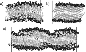
Figure 2: Snapshot of lipid bilayers a) fluid bilayer $L_{\alpha}$, b) tilted gel $L_{\beta^{\prime}}$ c) asymmetric ripple $P_{\beta^{\prime}}$

In our work, the solvent diameter was chosen $\sigma_{s}=\sigma_{h}$. Single head beads are soluble, (i.e., they do not demix with solvent) if the free solvent density is less than $\rho_{\mbox{\tiny free}}\sim 2.6/\sigma^{3}$. At sufficiently low temperatures, the lipids self-assemble into bilayers (see Fig. 2). The properties of these bilayers will be discussed in detail elsewhere lenz2 ; lenz3 . Here we just cite some of the main results. Like the monolayers, the bilayers exhibit a main transition. For small heads $(\sigma_{h}=0.9\sigma)$, the gel phase is untilted, i.e., we obtain an $L_{\alpha}$ phase. For larger heads $(\sigma_{h}=1.1\sigma)$, the structure of the gel phase depends on the free solvent density $\rho_{\mbox{\tiny free}}$. We note that the solvent entropically penalizes lipid/solvent interfaces and thus effectively creates an attractive depletion interaction between the beads next to these interface, i.e., the head beads. The strength of this interaction is proportional to $\rho_{\mbox{\tiny free}}$. At low $\rho_{\mbox{\tiny free}}$,  the gel phase is interdigitated ($L_{\beta}^{\mbox{\tiny int}}$), at moderate $\rho_{\mbox{\tiny free}}>1.2/\sigma^{3}$, it is tilted ($L_{\beta^{\prime}}$). Hence weak head attraction leads to the formation of the interdigitated phase, and moderate head attraction to the tilted gel phase, in agreement with experiments.

Most rewardingly, we also recover the ripple phase $P_{\beta^{\prime}}$ which intrudes between the tilted gel phase and the fluid phase. A snapshot is shown in Fig. 2 c). The two main experimental rippled states, the ‘asymmetric’ and the ‘symmetric’ rippled state, are recovered in simulations, with properties that are very similar to experimental properties lenz2 . A similar structure than that of our asymmetric ripple has been found recently in a (much more involved) atomistic simulation of a Lecithine bilayer devries . Our simulations show that this structure is generic, in the sense that it can be reproduced with a coarse-grained model, and that it is closely related to the structure of the corresponding symmetric rippled state lenz2 .

4 Conclusions and Outlook

To conclude, we have presented a versatile coarse-grained model that allows to study lipid monolayers and self-assembled bilayers and reproduces their most important internal phase transitions. It can be used to study a variety of questions related to membrane biophysics where atomic details do not matter, but the characteristic molecular features of lipids are still important. For example, we are currently applying it to study lipid-mediated interaction mechanisms between proteins An example snapshot is shown in Fig. 3.

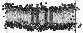
Figure 3: Fluid membrane with two embedded coarse-grained transmembrane proteins

Acknowledgements

We thank the NIC computing center in Jülich for computer time. This work was funded by the Deutsche Forschungsgemeinschaft.

Appendix: Technical Remarks

The Monte Carlo simulations described above were carried out at constant pressure $P$ with periodic boundary conditions in a simulation box of variable size and shape: The simulation box is a parallelepiped spanned by the vectors $(L_{x},0,0)$, $(s_{1}L_{x},L_{y},0)$, and $(s_{2}L_{x},s_{3}L_{y},L_{z})$. All $L_{\alpha}$ and $s_{i}$ are allowed to fluctuate. In addition, it is sometimes convenient to work in a semi-grand canonical ensemble with fluctuating number $N_{s}$ of solvent beads and given solvent chemical potential $\mu_{s}$. Hence we have three types of possible trial Monte Carlo moves:

• Moves that change the positions of beads.

• Moves that changes the volume and/or shape of the box: Random increments drawn randomly from a symmetric distribution with mean zero are added to $L_{\alpha}$ or $s_{i}$. All bead coordinates are rescaled accordingly.

• Moves that changes the number $N_{s}$ of solvent particles: We first decide with probability 1/2 whether to attempt a solvent removal or a solvent addition. Then, we choose randomly the particle to be removed, or the position of the particle to be added.

The moves are accepted or rejected according to one of the standard Monte Carlo schemes (e.g., Metropolis), with the effective Hamiltonian frenkel_book

$$H_{\mbox{\tiny eff}}=H\!+\!PV\!-\!\mu_{s}N_{s}\!-\!k_{B}T\ln\big{[}(V/V_{0})^{N}/N_{s}!\big{]},$$ (4)

where $H$ is the interaction energy, $V=L_{x}L_{y}L_{z}$ the volume of the simulation box, $V_{0}$ an arbitrary reference volume (e.g., $V_{0}=\sigma_{t}^{3}$), and $N$ the total number of beads (solvent and lipids). The $L_{\alpha}$ are not allowed to fall below a given threshold, otherwise the move is rejected.

We close with a remark on parallelization. For large scale applications, our Monte Carlo code has been parallelized geometrically. One commonly used spatial decomposition scheme for systems with short range interactions (see, e.g., the review heffelfinger ) proceeds as follows: The simulation box is divided into domains which are distributed on the processors. These are further subdivided into labelled subdomains such that subdomains with the same label are separated by a distance larger than the maximum interaction range. Subdomains with the same label are then processed in parallel. This algorithm is relatively straightforward, yet it has the drawback that it does not strictly fulfill detailed balance: Within a move for given subdomain label $\alpha$, particles can cross a subdomain boundary only in one direction (i.e., leaving the set of subdomains $\alpha$). If the different sets $\alpha$ are processed equally often, the final distribution is presumably not affected. Nevertheless, we feel uncomfortable with this method and favor a variant of a parallelization scheme recently proposed by Uhlherr et al. uhlherr . The idea is to define ‘active regions’ and assign them to different processors. A possible decomposition scheme is shown in Fig. 4. Only particles with centers in the active regions are moved, and moves that take a particle outside of its active region are rejected. To ensure that the algorithm remains ergodic, the active regions are periodically redefined. One easily checks that individual bead moves fulfill detailed balance. We note that the active regions must not necessarily have the same size, and furthermore moves in interesting regions can be more frequent. This feature makes the concept of ‘active regions’ interesting even for applications on scalar computers.

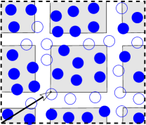
Figure 4: Sketch of the domain decomposition scheme used for the parallelization of the Monte Carlo algorithm (a variant of Uhlherr et al. uhlherr ). The system is covered with a grid of active regions (shaded rectangles, filled particles). The distance between active regions must exceed the interaction range between beads. The offset of the active grid (arrow) changes periodically and is chosen randomly.

References

References

- (1) R. B. Gennis, Biomembranes, Springer Verlag, New York, 1989.
- (2) R. Koynova, M. Caffrey, Chem. Phys. Lipids 69, 1 (1994); Biophys. Biochim. Acta 1376, 91 (1998).
- (3) V. M. Kaganer, H. Möhwald, P. Dutta, Rev. Mod. Phys. 71, 779 (1999).
- (4) D. Düchs, F. Schmid, J. Phys.: Cond. Matter 13, 4835 (2001).
- (5) C. Stadler, H. Lange, F. Schmid, Phys. Rev. E 59, 4248 (1999); C. Stadler, F. Schmid, J. Chem. Phys. 110, 9697 (1999).
- (6) O. Lenz, F. Schmid, J. Mol. Liquids 117, 147 (2004).
- (7) B. Smit et al., J. Phys. Chem. 94, 6933 (1990); R. Goetz, R. Lipowsky, J. Chem. Phys. 108, 7397 (1998); J. C. Shillcock, R. Lipowsky, J. Chem. Phys. 117, 5048 (2002); M. Kranenburg, J. P. Nicolas, B. Smit, Phys. Chem. Cehm. Phys. 6, 4142 (2004).
- (8) H. Noguchi, M. Takasu, Phys. Rev. E 64, 041913 (2001); O. Farago, J. Chem. Phys. 119, 596 (2004); I. R. Cooke, K. Kremer, M. Deserno, Phys. Rev. E 72, 011506 (2005).
- (9) O. Lenz, F. Schmid, submitted (2006) www.arxiv.org/abs/physics/0608146.
- (10) O. Lenz, F. Schmid, in preparation.
- (11) A. H. de Vries et al., PNAS 102, 5392 (1005).
- (12) D. Frenkel, B. Smit, Understanding Molecular Simulations, Academic Press, San Diego, 2002.
- (13) G. S. Heffelfinger, Comp. Phys. Comm. 128, 219 (2000).
- (14) A. Uhlherr et al., Comp. Phys. Comm. 144, 1 (2002).