The art of fitting financial time series with Lévy stable distributions

Abstract

This paper illustrates a procedure for fitting financial data with $\alpha$-stable distributions. After using all the available methods to evaluate the distribution parameters, one can qualitatively select the best estimate and run some goodness-of-fit tests on this estimate, in order to quantitatively assess its quality. It turns out that, for the two investigated data sets (MIB30 and DJIA from 2000 to present), an $\alpha$-stable fit of log-returns is reasonably good.

I Introduction

There are several stochastic models available to fit financial price or index time series $\{S_{i}\}_{i=1}^{N}$ bertram05 . Building on the ideas presented by Bachelier in his thesis bachelier00 ; cootner64 , in a seminal paper published in 1963, Mandelbrot proposed the Lévy $\alpha$-stable distribution as a suitable model for price differences, $\xi=S_{i+1}-S_{i}$, or logarithmic returns, $\xi_{\log}=\log(S_{i+1})-\log(S_{i})$ mandelbrot63 . In the financial literature, the debate on the Lévy $\alpha$-stable model focused on the infinite variance of the distribution, leading to the introduction of subordinated models mandelbrot67 ; clark73 ; merton90 ; in the physical literature, Mantegna used the model for the empirical analysis of historical stock-exchange indices mantegna91 . Later, Mantegna and Stanley proposed a “truncated” Lévy distribution mantegna94 ; mantegna95 ; koponen95 , an instance of the so-called KoBoL (Koponen, Boyarchenko and Levendorskii) distributions schoutens03 .

Lévy $\alpha$-stable distributions are characterized by a power-law decay with index $0<\alpha\leq 2$. Fitting the tails of an empirical distribution with a power law is not simple at all. Weron has shown that some popular methods, such as the log-log linear regression and Hill’s estimator, give biased results and overestimate the tail exponent for deviates taken from an $\alpha$-stable distribution weron01 .

In this paper, a method is proposed for fitting financial log-return time series with Lévy $\alpha$-stable distributions. It uses the program stable.exe developed by Nolan nolan99 and the Chambers-Mallow-Stuck algorithm for the generation of Lévy $\alpha$-stable deviates chambers76 ; weron96 ; mcculloch . The datasets are: the daily adjusted close for the DJIA index taken from http://finance.yahoo.com and the daily adjusted close for the MIB30 index taken from http://it.finance.yahoo.com both for the period 1 January 2000 - 3 August 2006. The two datasets and the program stable.exe are freely available, so that whoever can reproduce the results reported below and use the method on other datasets.

The definition of Lévy $\alpha$-stable distributions is presented in Section II. Section III is devoted to the results of the empirical analysis. A critical discussion of these results can be found in Section IV.

II Theory

A random variable $\Xi$ is stable or stable in the broad sense if, given two independent copies of $\Xi$, $\Xi_{1}$ and $\Xi_{2}$, and any positive constant $a$ and $b$, there exist some positive $c$ and some real $d$ such that the sum $a\Xi_{1}+b\Xi_{2}$ has the same distribution as $c\Xi+d$. If this property holds with $d=0$ for any $a$ and $b$ then $\Xi$ is called strictly stable or stable in the narrow sense. This definition is equivalent to the following one which relates the stable property to convolutions of distributions and to the generalization of the central limit theorem levy : A random variable $\Xi$ is stable if and only if, for all $n>1$ independent and identical copies of $\Xi$, $\Xi_{1},\ldots,\Xi_{n}$, there exist a positive constant $c_{n}$ and a real constant $d_{n}$ such that the sum $\Xi_{1}+\ldots+\Xi_{n}$ has the same distribution as $c_{n}\Xi+d_{n}$. It turns out that a random variable $\Xi$ is stable if and only if it has the same distribution as $aZ+b$, where $0<\alpha\leq 2$, $-1\leq\beta\leq 1$, $a>0$, $b\in\mathbb{R}$ and $Z$ is a random variable with the following characteristic function:

$$\langle\exp(i\kappa Z)\rangle=\exp\left(-|\kappa|^{\alpha}\left[1-i\beta\tan\left(\frac{\pi\alpha}{2}\right){\rm sign}(\kappa)\right]\right)\,\,{\rm if}\,\alpha\neq 1$$ (1)

and

$$\langle\exp(i\kappa Z)\rangle=\exp\left(-|\kappa|\left[1+i\beta\left(\frac{2}{\pi}\right){\rm sign}(\kappa)\log(|\kappa|)\right]\right)\,\,{\rm if}\,\alpha=1.$$ (2)

Thus, four parameters ($a$, $b$, $\alpha$, $\beta$) are needed to specify a general stable distribution. Unfortunately, the parameterization is not unique and this has caused several errors nolan98 . In this paper, a parameterization is used, due to Samorodnitsky and Taqqu taqqu94 :

$$\langle\exp(i\kappa\Xi)\rangle=\exp\left(-\gamma^{\alpha}|\kappa|^{\alpha}\left[1-i\beta\tan\left(\frac{\pi\alpha}{2}\right){\rm sign}(\kappa)\right]+i\delta\kappa\right)\,\,{\rm if}\,\alpha\neq 1$$ (3)

and

$$\langle\exp(i\kappa\Xi)\rangle=\exp\left(-\gamma|\kappa|\left[1+i\beta\left(\frac{2}{\pi}\right){\rm sign}(\kappa)\log(|\kappa|)\right]+i\delta\kappa\right)\,\,{\rm if}\,\alpha=1.$$ (4)

This parameterization is called $S1$ in stable.exe. The program uses a different parameterization (called $S0$) for numerical calculations:

$$\langle\exp(i\kappa\Xi_{0})\rangle=\exp\left(-\gamma^{\alpha}|\kappa|^{\alpha}\left[1-i\beta\tan\left(\frac{\pi\alpha}{2}\right){\rm sign}(\kappa)\right]+i\left[\delta_{0}-\beta\tan\left(\frac{\pi\alpha}{2}\right)\right]\kappa\right)\,\,{\rm if}\,\alpha\neq 1$$ (5)

and

$$\langle\exp(i\kappa\Xi_{0})\rangle=\exp\left(-\gamma|\kappa|\left[1+i\beta\left(\frac{2}{\pi}\right){\rm sign}(\kappa)\log(|\kappa|)\right]+i\left[\delta_{0}-\beta\left(\frac{2}{\pi}\right)\gamma\log\gamma\right]\kappa\right)\,\,{\rm if}\,\alpha=1.$$ (6)

The above equations are modified versions of Zolotarev’s parameterizations zolotarev . Notice that in Eqs. (3) and (4), the scale $\gamma$ is positive and the location parameter $\delta$ has values in $\mathbb{R}$.

III Results

Daily values for the MIB30 and DJIA adjusted close have been downloaded from http://it.finance.yahoo.com and http://finance.yahoo.com, respectively, for the period 1 January 2000 - 3 August 2006 adjusted . The MIB30 is an index comprising 30 “blue chip” shares on the Italian Stock Exchange, whereas the DJIA is a weighted average of the prices of 30 industrial companies that are representative of the market as a whole. Notice that the MIB30 includes non-industrial shares. Therefore, the two indices cannot be used for comparisons on the behaviour of the industrial sector in Italy and in the USA. Moreover, the composition of indices varies with time, making it problematic to compare different historical periods. However, the following analysis concerns the statistical properties of the two indices, considered representative of the stock-exchange average trends. The datasets are presented in Figs 1-4. Figs. 1 and 2 report the index value as a function of trading day. There are 1709 points in the MIB30 dataset and 1656 points in the DJIA dataset. Correpondingly, there are 1708 MIB30 log-returns and 1655 DJIA log-returns. They are represented in Figs. 3 and 4, respectively. The intermittent behaviour typical of log-return time series can be already detected by eye inspection of Figs. 3 and 4, but this property will not be further studied.

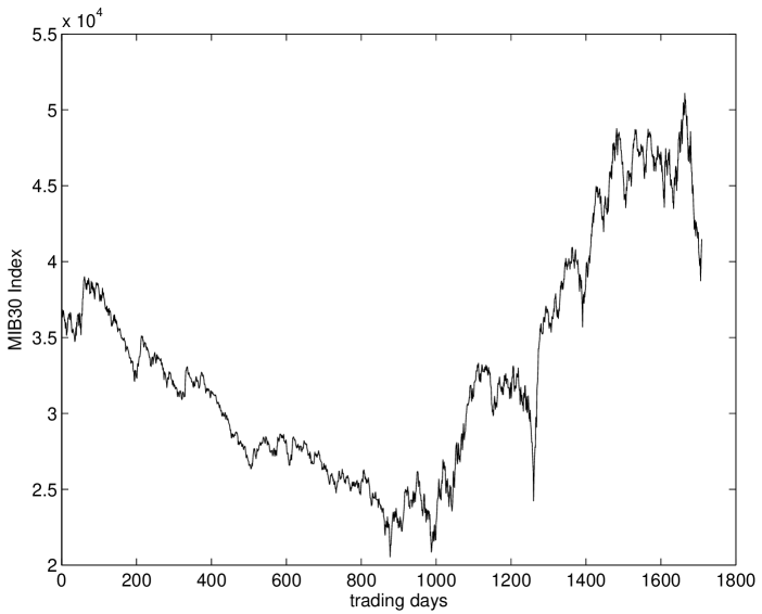
Figure 1: MIB30: Adjusted close time series.

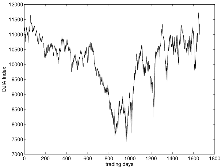
Figure 2: DJIA: Adjusted close time series.

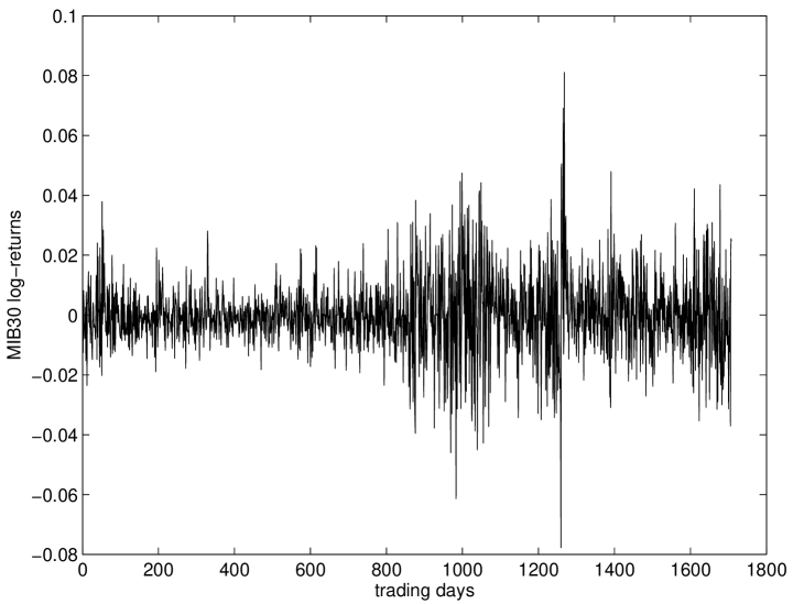
Figure 3: MIB30: Log-return time series.

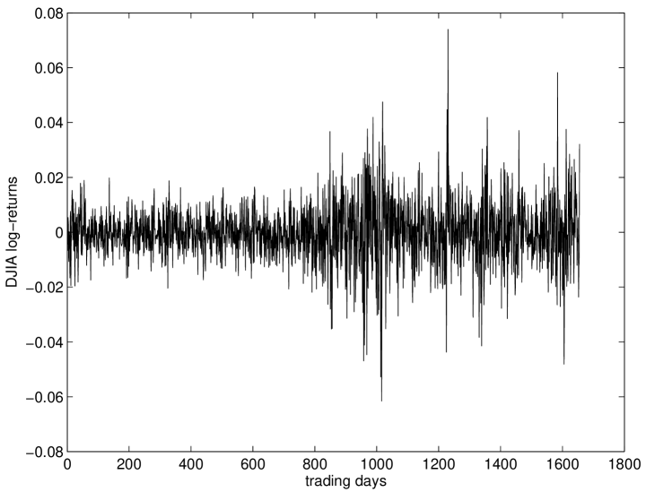
Figure 4: DJIA: Log-return time series.

In Table I, the mean, variance, skewness, and kurtosis are reported for both the MIB30 and the DJIA log-return time series.

Table 1: Mean, variance, skewness, and kurtosis of the two log-return time series.

Index	Mean	Variance	Skewness	Kurtosis
MIB30	$7.3\cdot 10^{-5}$	$1.6\cdot 10^{-4}$	0.22	6.7
DJIA	$6.1\cdot 10^{-6}$	$1.3\cdot 10^{-4}$	0.038	6.6

The two log-return time series were given as input to stable.exe. The program implements three methods for the estimate of the four parameters of Eqs. (3) and (4). The first one is based on a maximum likelihood (ML) estimator nolan99 ; dumouchel83 . The second method uses tabulated quantiles (QB) of Lévy $\alpha$-stable distributions mcculloch86 and it is restricted to $\alpha\geq 0.6$. Finally, in the third method, a regression on the sample characteristic (SC) function is used koutrouvelis ; kogon .

In Table II, the estimated values of $\alpha$, $\beta$, $\gamma$, and $\delta$ are reported. The estimates were obtained with the standard settings of stable.exe.

Table 2: Estimated parameters of the $\alpha$-stable distribution.

Method	$\alpha$	$\beta$	$\gamma$	$\delta$
MIB30
ML	1.57	0.159	$6.76\cdot 10^{-3}$	$3.50\cdot 10^{-4}$
QB	1.42	0.108	$6.23\cdot 10^{-3}$	$5.43\cdot 10^{-4}$
SC	1.72	0.263	$7.06\cdot 10^{-3}$	$2.53\cdot 10^{-4}$
DJIA
ML	1.73	0.014	$6.60\cdot 10^{-3}$	$4.43\cdot 10^{-5}$
QB	1.60	-0.004	$6.21\cdot 10^{-3}$	$2.69\cdot 10^{-4}$
SC	1.81	0.129	$6.69\cdot 10^{-3}$	$1.79\cdot 10^{-4}$

In order to preliminary assess the quality of the fits, three synthetic series of log-returns for each index were generated with the Chambers-Mallow-Stuck algorithm. The empirical complementary cumulative distribution function (CCDF) for absolute log-returns was compared with the simulated CCDFs, see Figs. 5 and 6. In both cases, the fit based on the SC function turned out to be the best one. A refinement of the ML method gave the same values for the four parameters as the SC algorithm. Therefore, the SC result was selected as the null hypothesis for two standard quantitative goodness-of-fit tests: The one-sided Kolmogorov-Smirnov (KS) test and the $\chi^{2}$ test.

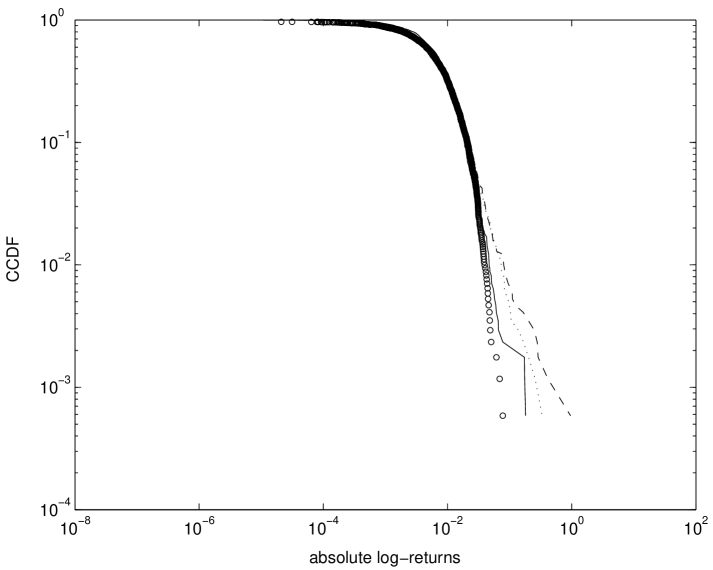
Figure 5: MIB30: Comparison of CCDFs for absolute log-returns. Circles: Empirical data. Dotted line: Maximum-likelihood fit. Dashed line: Quantile based fit. Solid line: Fit based on the SC function.

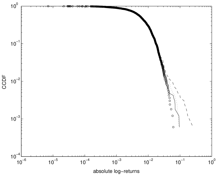
Figure 6: DJIA: Comparison of CCDFs for absolute log-returns. Circles: Empirical data. Dotted line: Maximum-likelihood fit. Dashed line: Quantile based fit. Solid line: Fit based on the SC function.

For the KS test, the range of MIB30 log-returns, $(-0.0777,\,0.0811)$, was divided into 1654 intervals of width $9.6\times 10^{-5}$. Then the number of points lying in each interval was counted and partially summed starting from $-0.0777$, leading to an estimate of the empirical cumulative distribution function (CDF). The same procedure was used for DJIA log-returns. In this case the range was $(-0.0615,\,0.0740)$, the number of intervals 1693, and their width $8.0\times 10^{-5}$. In Figs. $7$ and $8$, the empirical CDF is plotted together with the theoretical CDF obtained from the fit based on the SC function. For large sample sizes, the one-sided KS parameter, $D$, is approximately given by:

$$D=\max(|{\rm CDF}_{i}-{\rm CDFth}_{i}|),$$

where ${\rm CDF}_{i}$ and ${\rm CDFth}_{i}$ are, respectively, the empirical and the theoretical values corresponding to the $i-$th bin; at $5\%$ significance, $D$ can be compared with the limiting value $d=1.36/\sqrt{N}$, where $N$ is the number of empirical CDF points. For MIB30 log-returns $D=0.0387$ and $d=0.0334$, whereas for DJIA log-returns $D=0.0232$ and $d=0.0330$. Therefore, the null hypothesis of $\alpha$-stable distributed log-returns can be rejected for the MIB30, but not for the DJIA data.

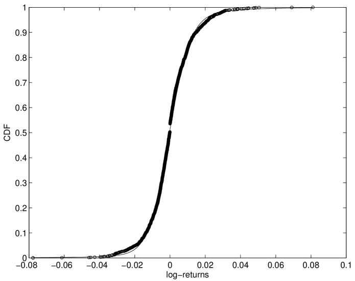
Figure 7: MIB30: Comparison of CDFs for log-returns. Circles: Empirical data. Solid line: Fit based on the SC function.

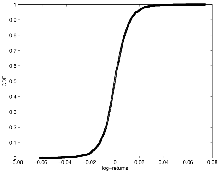
Figure 8: DJIA: Comparison of CDFs for log-returns. Circles: Empirical data. Solid line: Fit based on the SC function.

For the $\chi^{2}$ test, the range of MIB30 and DJIA log-returns was divided into 30 equal intervals. Then, the observed $O_{i}$ and expected $E_{i}$ number of points lying in each interval were evaluated; these data are plotted in Figs. 9 and 10. After aggregating the intervals with $E_{i}<5$, $\bar{\chi}^{2}$ was obtained from the formula:

$$\bar{\chi}^{2}=\sum_{i}\frac{(O_{i}-E_{i})^{2}}{E_{i}}$$

The number of degrees of freedom is given by the number of intervals where $E_{i}\geq 5$ minus 5 (4 estimated parameters and the normalization). For MIB30 data, $\bar{\chi}^{2}=91.5$ with 10 degrees of freedom. The probability that $\chi^{2}>\bar{\chi}^{2}$ is 0. For the DJIA time series, $\bar{\chi}^{2}=26.8$ with 11 degrees of freedom. The probability that $\chi^{2}>\bar{\chi}^{2}$ is 0.005. Again, for DJIA data, even if at a low significance level, the null hypothesis may be accepted.

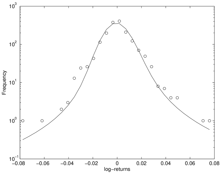
Figure 9: MIB30: Comparison of PDFs for log-returns. Circles: Empirical data. Solid-line: Fit based on the SC function.

Figure 10: DJIA: Comparison of PDFs for log-returns. Circles: Empirical data. Solid-line: Fit based on SC function.

IV Conclusions and outlook

This paper illustrates a procedure for fitting financial data with $\alpha$-stable distributions. The first step is to use all the available methods to evaluate the four parameters $\alpha$, $\beta$, $\gamma$, and $\delta$. Then, one can qualitatively select the best estimate and run some goodness-of-fit tests, in order to quantitatively assess the quality of the fit.

The main conclusion of this paper is that, for the investigated data sets, an $\alpha$-stable fit is not so bad; the best parameter estimate is obtained with a method based on a sample characteristic function fit. Incidentally, the tail index, $\alpha$, is 1.72 for MIB30 and 1.81 for DJIA. These values are consistent with previous results rachev00 and with remarks made by Weron weron01 . The performance in two standard goodness-of-fit tests (KS and $\chi^{2}$) is better for DJIA data.

The two hypothesis tests used in this paper have some limitations. For instance, the KS test is more sensitive to the central part of the distribution and underestimates the tail contribution. For this reason, it would be better to use the Anderson-Darling (AD) test stephens74 . However, a standardized AD test is not available for $\alpha$-stable distributions. Moreover, the value of $\bar{\chi}^{2}$ in the $\chi^{2}$ test is sensitive to the choice of intervals, and a detailed analysis on this dependence would be necessary.

Given a set of financial log-returns, is it possible to find the best-fitting distribution? In general this question is ill-posed. As mentioned in the introduction, there are several possible competing distributions that can give very similar results in the interval of interest. Moreover, depending on the specific criterion chosen, different distributions may turn out to be the best according to that criterion. Therefore, if there is no theory suggesting the choice of a specific distribution, it is advisable to use a pragmatic and heuristic approach, application-oriented. For example, Figs. 9 and 10 show that the Lévy $\alpha$-stable fit discussed in this paper tends to underestimate the tails of the probability density function (PDF) in the two investigated cases. In risk asessment procedures, such as value at risk estimates, this may be an undesirable feature, and it could be wiser to look for some other probability density whose the PDF prudentially overestimates the tail region.

References

- (1) W. Bertram, Modelling asset dynamics via an empirical investigation of Australian Stock Exchange data, Ph.D Thesis, School of Mathematics and Statistics, University of Sydney, 2005.
- (2) L. Bachelier, Théorie de la spéculation, Gauthier-Villar, Paris, 1900. (Reprinted in 1995, Editions Jacques Gabay, Paris).
- (3) P.H. Cootner (Ed.), The Random Character of Stock Market Prices, MIT Press, Cambridge, MA, 1964.
- (4) B. Mandelbrot, The Variation of Certain Speculative Prices, The Journal of Business 36, 394–419 (1963).
- (5) B. Mandelbrot, H.M. Taylor, On the distribution of stock price differences, Oper. Res. 15 1057 -1062 (1967).
- (6) P.K. Clark, A subordinated stochastic process model with finite variance for speculative prices, Econometrica 41, 135 -156 (1973).
- (7) R.C. Merton, Continuous Time Finance, Blackwell, Cambridge, MA, 1990.
- (8) R.N. Mantegna, Lévy walks and enhanced diffusion in Milan stock exchange, Physica A 179, 232–242 (1991).
- (9) R.N. Mantegna and H.E. Stanley, Stochastic Process With Ultra-Slow Convergence to a Gaussian: The Truncated Lévy Flight, Phys. Rev. Lett. 73, 2946–2949 (1994).
- (10) R.N. Mantegna and H.E. Stanley, Scaling behaviour in the dynamics of an economic index, Nature 376, 46–49 (1995).
- (11) I. Koponen, Analytic approach to the problem of convergence of truncated Lévy flights towards the Gaussian stochastic process, Phys. Rev. E 52, 1197–1199 (1195).
- (12) W. Schoutens, Lévy Processes in Finance: Pricing Financial Derivatives, Wiley, New York, NY, 2003.
- (13) R. Weron, Lévy-stable distributions revisited: tail index does not exclude the Lévy stable regime, Int. J. Mod. Phys. C 12, 209–223 (2001).
- (14) J.P. Nolan, Fitting data and assessing goodness-of-fit with stable distributions, in J. P. Nolan and A. Swami (Eds.), Proceedings of the ASA- IMS Conference on Heavy Tailed Distributions, 1999. J.P. Nolan, Maximum likelihood estimation of stable parameters, in O.E. Barndorff-Nielsen, T. Mikosch, and S. I. Resnick (Eds.), Lévy Processes: Theory and Applications, Birkhäuser, Boston, 2001. The program stable.exe can be downloaded from http://academic2.american.edu/jpnolan/stable/stable.html.
- (15) J.M. Chambers, C.L. Mallows, B.W. Stuck, A Method for Simulating Stable Random Variables J. Amer. Stat. Assoc. 71, 340–344 (1976).
- (16) R. Weron, On the Chambers-Mallows-Stuck Method for Simulating Skewed Stable Random Variables, Statist. Probab. Lett. 28, 165–171 (1996). R. Weron, Correction to: On the Chambers-Mallows-Stuck Method for Simulating Skewed Stable Random Variables, Research report, Wrocław University of Technology, 1996.
- (17) Various implementations of the Chambers-Mallows-Stuck algorithm are available from the web page of J. Huston McCulloch: http://www.econ.ohio-state.edu/jhm/jhm.html.
- (18) P. Lévy, Théorie de l’addition de variables aléatoires, Editions Jacques Gabay, Paris, 1954.
- (19) J.P. Nolan, Parameterizations and modes of stable distributions, Statist. Probab. Lett. 38, 187–195 (1998).
- (20) G. Samorodnitsky and M.S. Taqqu, Stable Non-Gaussian Random Processes, Chapman & Hall, New York, NY, 1994.
- (21) A. Zolotarev, One-Dimensional Stable Distributions, American Mathematical Society, Providence, RI, 1986.
- (22) The adjusted close is the close index value adjusted for all splits and dividends. See http://help.yahoo.com/help/us/fin/quote/quote-12.html for further information.
- (23) W.H. DuMouchel, Estimating the Stable Index in Order to Measure Tail Thickness: A Critique, Ann. Statist. 11, 1019–1031 (1983).
- (24) J.H. McCulloch. Simple Consistent Estimates of Stable Distribution Parameters, Commun. Statist. - Simula. 15, 1109-1136 (1986).
- (25) I.A. Koutrouvelis, Regression-Type Estimation of the Parameters of Stable Laws, J. Amer. Statist. Assoc. 75, 918–928 (1980). I.A. Koutrouvelis, An Iterative Procedure for the Estimation of the Parameters of the Stable Law, Commun. Statist. - Simula. 10 17–28 (1981).
- (26) S.M. Kogon, D.B. Williams, Characteristic function based estimation of stable parameters, in R. Adler, R. Feldman, and M. Taqqu, eds., A Practical Guide to Heavy Tails, Birkäuser, Boston, MA, 1998.
- (27) S. Rachev and S. Mittnik, Stable Paretian Models in Finance, Wiley, New York, NY, 2000.
- (28) M.A. Stephens, EDF Statistics for Goodness of Fit and Some Comparisons, J. Amer. Stat. Assoc. 69, 730–737 (1974).