Extract Signals by Fitting $\chi^{2}$ Distribution of the Kinematic Fit

Abstract

In measuring the $\psi(2S)$ radiative decays at BESII, contribution of the background is serious in most of the final states. To extract the number of signal events, a fit to the $\chi^{2}$ distribution of kinematic fit using signal and background components is proposed. Extensive Monte-Carlo simulations (MCS) are performed, and the results show that the shape of $\chi^{2}$ distribution of the signal channel looks different from those of the background channels, thus it provides us by fitting the $\chi^{2}$ distribution of the data to extract the number of signal events. An input-output test is performed using MCS, and the uncertainty of the fit method is found to be less than 2%.

I INTRODUCTION

The radiative decays of $J/\psi$ and $\psi^{\prime}$, due to the direct coupling of outgoing photon to the charm quark, could be an excellent laboratory to study the hadron spectroscopy and search for exotic states. At the leading order of pQCD picture, both the $J/\psi$ and $\psi$ radiative decays can be described by the $c\bar{c}$ quark annihilation with the emission of one photon and two gluons. There could be a possibility that the two gluons might form a glueball, or one gluon combines with a $q\bar{q}$ pair to form a hybrid state, or the two gluons couple to a multiquark state. Compared with $J/\psi$ decays, few measurements of $\psi(2S)$ radiative decays have been reported pdg2004 . BESII detector has accumulated 14 million $\psi(2S)$ events, and it offers an opportunity to study a number of $\psi(2S)$ radiative decays.

Experimentally, an event is reconstructed by using the detector information on charged tracks and photons. For removing background events, the constraints of the energy and momentum conservation for the final state of the signal channel are imposed on the fitting to the 4-component momentum (4C) reconstructed by the detector, and the background events can be suppressed by using information of the distribution of the $\chi^{2}$ of the fit. With the help of the Monte-Carlo simulation, a reasonable requirement on $\chi^{2}$ can be obtained by comparing the $\chi^{2}$ distributions between the signal and the background channels. However, the $\chi^{2}$ cut method fails badly sometimes if the $\chi^{2}$ distribution of the background channel overlaps largely with the signal channels. In this paper, we try to fit the $\chi^{2}$ distribution to extract the number of signal events in measuring the exclusive decays of $\psi(2S)\to\gamma+\textrm{hadrons}$ at BESII detector, which includes 2, 4 and 6 prongs (stable hadron—pion,kaon,proton or anti-proton).

II Fit to the $\chi^{2}$ distribution

Monte Carlo simulation shows that backgrounds of the radiative decay of $\psi(2S)\to\gamma+\textrm{hadrons}$ are largely coming from multi-photon decay channels, namely, the dominant background is $\psi(2S)\to\pi^{0}+\textrm{hadrons}$, and some contaminations are from $\psi(2S)\to\gamma\pi^{0}+\textrm{hadrons}$, along with other possible backgrounds. In principle, their $\chi^{2}$ distributions of the kinematic fit can be obtained with MCS. Since these types of backgrounds are due to missing photons, their distributions of the $\chi^{2}$ shapes are different from each other. This property allows us to express the observed $\chi^{2}$ distributions of the data sample by that of the signal channel and the background channels, $i.e.$

$$\chi^{2}_{obs}=w_{s}\chi^{2}_{sig}+\sum_{w_{b_{i}}}w_{b_{i}}\chi^{2}_{bg},$$ (1)

where $w_{s}$ and $w_{b_{i}}$ are the weight of the signal and the background decays, respectively. If the background channels are completely known, then the signal events can be extracted reliably by fitting to the data with Equation (1).

III Monte Carlo Simulation

III.1 Background

To make the measurement of $\psi^{\prime}$ radiative decays reliable, the background should be fully studied. With the help of SIMBES system simbes , extensive simulations have been performed. Table 1 summarizes the possible background contributions to signal mode $\psi(2S)\to\gamma+\textrm{hadrons}$. Generally speaking, the dominant backgrounds come from multi-photon decays, i.e. $\psi(2S)\to n\gamma+\textrm{hadrons}~{}(n\geq 2)$. With more missing photons in background decays, the contamination to the signal decay becomes lower and lower.

Tab. 1: The backgrounds for the radiative decay $\psi(2S)\to\gamma+\textrm{hadrons}$, where the normalized background events are based on 14M $\psi(2S)$ events and the branching fractions given in PDG table with requirement $m_{\textrm{hadrons}}<3.0$ GeV.

Signal mode	Background modes	$N_{bg}$(normalized)
$\psi(2S)\to$	$\psi(2S)\to$
$\gamma p\bar{p}$	$\pi^{0}p\bar{p}$	$141.5$
	$\gamma\pi^{0}p\bar{p}$	$8.8$
$\gamma K^{+}K^{-}\pi^{+}\pi^{-}$	$\pi^{0}K^{+}K^{-}\pi^{+}\pi^{-}$	$98$
	$\gamma\pi^{0}K^{+}K^{-}\pi^{+}\pi^{-}$	$16$
$\gamma 2(\pi^{+}\pi^{-})$	$\pi^{0}2(\pi^{+}\pi^{-})$	805.0
	$\pi^{+}\pi^{-}J/\psi,J/\psi\to 3\pi$	33.4
$\gamma K^{+}K^{-}2(\pi^{+}\pi^{-})$	$\pi^{0}K^{+}K^{-}2(\pi^{+}\pi^{-})$	6.0
	$\gamma\pi^{0}K^{+}K^{-}2(\pi^{+}\pi^{-})$	6.1

III.2 $\chi^{2}$ distribution

Figure 1 shows the shapes of $\chi^{2}$ distributions for $\psi(2S)\to\gamma+\textrm{hadrons}$ after data selection. In plots the points with error bars are the signal decays into $\gamma p\bar{p}~{}(a)$, $\gamma K^{+}K^{-}\pi^{+}\pi^{-}~{}(b)$, $\gamma 2(\pi^{+}\pi^{-})~{}(c)$ and $\gamma K^{+}K^{-}2(\pi^{+}\pi^{-})~{}(d)$, respectively. The dashed histograms and the solid line histograms correspond to the distributions of the background channels $\psi(2S)\to\pi^{0}+\textrm{hadrons}$ and $\gamma\pi^{0}+\textrm{hadrons}$, respectively. For comparison of their shapes, the background events are respectively normalized to signal events. Obviously it can be seen that the shapes of the signal $\chi^{2}$ distributions are different from those of the background modes. This could be understandable due to the fact that the expectation of the $\chi^{2}$ value of the kinematic fit becomes larger to the backgrounds originated from one or more photons missing.

Fig. 1: The chisqured distribution of MC samples for $\psi(2S)\to\gamma+\textrm{hadrons}$, where points with error bars show the $\chi^{2}$ shapes for $\textrm{hadrons}=p\bar{p}~{}(a),~{}K^{+}K^{-}\pi^{+}\pi^{-}~{}(b),~{}2(\pi^{+}\pi^{-})~{}(c)$ and $K^{+}K^{-}2(\pi^{+}\pi^{-})~{}(d)$, and the dashed histograms correspond to $\psi(2S)\to\pi^{0}+\textrm{hadrons}$ and the solid line histograms to $\psi(2S)\to\gamma\pi^{0}+\textrm{hadrons}$, respectively.

III.3 Input-output check of $\chi^{2}$ fit method

Since the dominant backgrounds of $\psi(2S)$ radiative decays originate from the photon missing decays, and their shapes are different from each other, therefore, fitting the $\chi^{2}$ distribution of the data with Equation (1) provides us a tool to extract the signal events. We employ MCS to make an input-output check and estimate the uncertainty of the $\chi^{2}$ fit method.

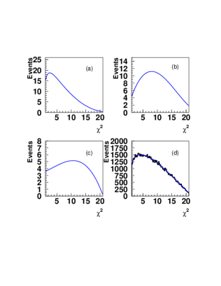
Fig. 2: The $\chi^{2}$ distribution for $\psi(2S)$ decays into the signal mode $\gamma K^{+}K^{-}\pi^{+}\pi^{-}$ (a), and the dominant background $\pi^{0}K^{+}K^{-}\pi^{+}\pi^{-}$ (b) and other unknown background (c). In plot (d) the histogram corresponds to the $\chi^{2}$ distribution of the sample generated with $\chi^{2}$ shapes in (a), (b) and (c) and the solid line to the fitted results with these $\chi^{2}$ components.

Figure 2 shows the $\chi^{2}$ distributions of the MC sample for $\psi(2S)$ decays into $\gamma K^{+}K^{-}\pi^{+}\pi^{-}$ (a), $\pi^{0}K^{+}K^{-}\pi^{+}\pi^{-}$ (b) and other unknown backgrounds by using 14M $\psi(2S)$ Lund-Charm MC sample. In order to make an input-output check of the $\chi^{2}$ fit method, a MC sample is generated with the $\chi^{2}$ shapes given in (a), (b) and (c) with an input number $N_{\textrm{sig}}^{\textrm{in}}$, $N_{\textrm{bg}}^{\textrm{in}}$ and $N_{\textrm{un}}^{\textrm{in}}$, respectively. Then we extract the numbers of events of these modes by the $\chi^{2}$ fit method. The total uncertainty includes errors from the $\chi^{2}$ fit method and the statistics, i.e.

$$\sigma_{\chi^{2}}=\sqrt{\left({N_{\textrm{sig}}^{\textrm{out}}-N_{\textrm{sig}}^{\textrm{in}}\over N_{\textrm{sig}}^{\textrm{in}}}\right)^{2}+\sigma_{\textrm{st}}^{2}},$$ (2)

where $N_{\textrm{sig}}^{\textrm{out}}$ is the number of the signal events obtained by the $\chi^{2}$ fit method, and $\sigma_{\textrm{st}}$ is the statistical uncertainty. Due to the uncertainty of the unknown background shape, we also consider the unknown background shape changed between the shape as shown in Figures 2 (b) and (c) parameterized by

$$\chi^{2}_{\textrm{un}}\to(1-x)\chi^{2}_{\textrm{un}}+x\chi^{2}_{\textrm{bg}},$$

where $\chi^{2}_{\textrm{un}}$ and $\chi^{2}_{\textrm{bg}}$ are the $\chi^{2}$ distribution of the unknown background and the dominant background, respectively. The $x$ value is taken between zero to one. The MCS shows that if the $\chi^{2}$ shape of the unknown background tends to that of the dominant background, the uncertainty of extracting the number of the dominant background becomes large by $\chi^{2}$ fit method. However, this situation does not worsen the signal uncertainty. The MCS with a large statistics shows that the uncertainty of the $\chi^{2}$ fit method is less than 2%.

IV SUMMARY

Based on MCS, it is found that the backgrounds of the $\psi(2S)$ decays into $\gamma+\textrm{hadrons}$ dominantly originate from the missing photon decays like $\psi(2S)\to n\gamma+\textrm{hadrons}~{}(n\geq 2)$. The $\chi^{2}$ distribution shapes of backgrounds are distinctive from those of the signal decays. This property allows us to extract the number of the signal events by the fit to the $\chi^{2}$ distribution. The results of MCS study indicate that the uncertainty of the extracted signal events from the method is less than 2%.

- (1) Particl Data Group, Phys. Lett. B, 2004, 592: 61.
- (2) Ablikim M., et al., BES Collab. Nucl. Instrum. Methods, 2005 A552: 344.