Gaussian Models for the Statistical Thermodynamics of Liquid Water

Abstract

A gaussian distribution of binding energies, but conditioned to exploit generally available information on packing in liquids, provides a statistical-thermodynamic theory of liquid water that is structurally non-committal, molecularly realistic, and surprisingly accurate. Neglect of fluctuation contributions to this gaussian model yields a mean-field theory that produces useless results. A refinement that accounts for sharper-than-gaussian behavior at high binding energies recognizes contributions from a discrete number of water molecules and permits a natural matching of numerically exact results. These gaussian models, which can be understood as vigorous simplifications of quasi-chemical theories, are applicable to aqueous environments where the utility of structural models based on geometrical considerations of water hydrogen bonding have not been established.

A widely accepted molecular-scale understanding of liquid water under physiological conditions has evolved over recent decades based upon the concept of promiscuous hydrogen-bonding that results in a thoroughly networked fluid Stillinger (1980). This view rests upon extensive molecular-scale simulation validated with traditional experimentation, and communicated with molecular-graphics tools. But water is a peculiar liquid. For example, the van der Waals theory Widom (1967), which provides the firmest basis for theories of simple liquids, is unsatisfactory for liquid water. Fig. 1 shows one experimental demonstration of that point. The foremost task in applying molecular statistical mechanical theory to liquid water is to address the equation-of-state distinctions exemplified in Fig. 1 on the basis of realistic intermolecular interactions. One theoretical approach is to accept the voluminous data that can be generated in a typical, realistic molecular simulation, but to craft a concise, quantitative statistical description of the basic thermodynamic characteristics Hummer et al. (1996); Ashbaugh and Pratt (2006). As exemplified below, those statistical theories can be concise indeed, and general in scope.

The focus here is analyzing the probability density distribution, $p(\varepsilon)$, of binding energies, $\varepsilon$, exhibited by a water molecule in liquid water. Thermodynamic properties are typically sensitive to the tails of this distribution, As a topical example, note that the population of weakly bound water molecules in liquid water can be decisive in filling transitions of carbon nanotubes Hummer et al. (2001). Thus, it can be helpful to have a clear idea how those weakly bound populations can be analyzed, and a focus of this work is the analysis of $p(\varepsilon)$.

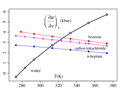
Figure 1: $\left(\partial u/\partial v\right)_{T}$ for several solvents as a function of temperature along the vapor saturation curve. For van der Waals liquids $\left(\partial u/\partial v\right)_{T}\approx a\rho^{2}$. Organic solvents conform to this expectation, but water is qualitatively different. The data are from Rowlinson and Swinton (1982).

Our motivation for the present analysis is the observation of severely non-gaussian $p(\varepsilon)$ in cases where repulsive interactions are prominent contributors Asthagiri et al. (2006). In such cases, conditioning to separate out effects of repulsive interactions was found to yield conditional distributions, $p\left(\varepsilon|r\geq\lambda\right)$, that were accurately gaussian. The idea is to account separately for close molecular encounters; then the direct statistical problem of evaluating the distribution of binding energies need only consider the fraction of the sample for which the distance to the nearest solvent molecule center, $r$, is greater than the conditioning radius $\lambda$. That fraction is $p\left(r\geq\lambda\right)$, the marginal probability. In previous quasi-chemical treatments, the marginal probability $p\left(r\geq\lambda\right)$ was denoted by $x_{0}$ Asthagiri et al. (2003); Paliwal et al. (2006); Asthagiri et al. (2006); Paulaitis and Pratt (2002).

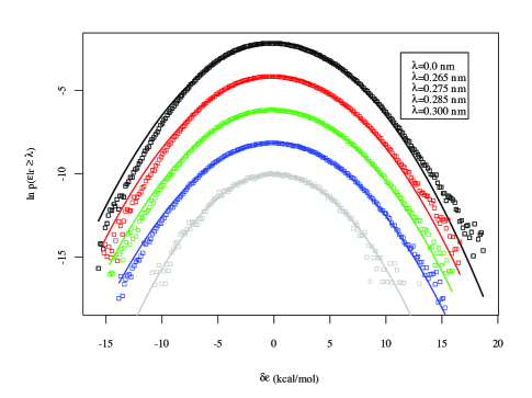
Figure 2: Probability density $p(\varepsilon|r\geq\lambda)$ of the binding energy of a water molecule in liquid water at 298 K. $\lambda$ = 0.0, …0.300 nm, from top to bottom with successive results shifted incrementally shifted downward by 2 for clarity. The solid lines are the gaussian model for each data set.

To follow that path, we seek $\mu^{\mathrm{{ex}}}$, the chemical potential of water in excess of the ideal contribution at the same density and temperature. On the basis of simulation data, we consider evaluating $\mu^{\mathrm{{ex}}}_{\mathrm{{HS}}}$, the excess chemical potential of a hard sphere solute, relative to $\mu^{\mathrm{{ex}}}$. The potential distribution theorem (PDT) Asthagiri et al. (2006); Beck et al. (2006); Paulaitis and Pratt (2002) then yields

$$e^{-\beta(\mu^{\mathrm{{ex}}}_{\mathrm{{HS}}}-\mu^{\mathrm{{ex}}})}=p\left(r\geq\lambda\right)\int\limits_{-\infty}^{+\infty}p\left(\varepsilon|r\geq\lambda\right)e^{\beta\varepsilon}\mathrm{d}\varepsilon~{}.$$ (1)

The thermodynamic temperature is $T=1/k_{B}\beta$ where $k_{B}$ is the Boltzmann’s constant. Since $\mu^{\mathrm{{ex}}}_{\mathrm{{HS}}}$ is known Ashbaugh and Pratt (2006), Eq. (1) gives $\mu^{\mathrm{{ex}}}$. We regard this conditioning as a regularization of the statistical problem embodied in Eq. (1) when $\lambda\rightarrow 0$, which is practically impossible on the basis of a direct, single calculation. After regularization, the statistical problem becomes merely difficult. A gaussian distribution model for $p\left(\varepsilon|r\geq\lambda\right)$ should be accurate when $\lambda\rightarrow\infty$, since then many solution elements will make small, weakly-correlated contributions to $\varepsilon$. The marginal probability $p\left(r\geq\lambda\right)$ becomes increasingly difficult to evaluate as $\lambda$ becomes large, however. For $\lambda$ on the order of molecular length scales typical of dense liquids, a simple gaussian model would accept some approximation error as the price for manageable statistical error. If $p\left(\varepsilon|r\geq\lambda\right)$ is modeled by a gaussian of mean $\left<\varepsilon|r\geq\lambda\right>$ and variance $\left<\delta\varepsilon^{2}|r\geq\lambda\right>$, then

$$\mu^{\mathrm{{ex}}}-\mu^{\mathrm{{ex}}}_{\mathrm{{HS}}}-kT\ln p\left(r\geq\lambda\right)-\left<\varepsilon|r\geq\lambda\right>=\\ \frac{1}{2kT}\left<\delta\varepsilon^{2}|r\geq\lambda\right>~{}.$$ (2)

This simple model motivates the following analyses.

To test these ideas, simulation data for liquid water was generated at 298, 350, and 400 K and 1 bar using methods described in Paliwal et al. (2006). The hard-sphere excess chemical potential was obtained from Ashbaugh and Pratt (2006). The distributions observed for $T$ = 298 K are shown in Fig 2. Table 1 collects the individual terms for the gaussian model, Eq. (2), at each temperature. The observed dependence on $\lambda$ of the free energy at each temperature is shown in Fig 3.

Fig. 2 shows that the unconditioned distribution $p\left(\varepsilon\right)$ displays positive skew, but the conditioning diminishes that skew perceptibly, as expected. $p\left(\varepsilon|r\geq\lambda\right)$ is least skewed for the largest $\lambda$, though the sample used is smaller by the fraction $p\left(r\geq\lambda\right)$, and thus less of the tail region is available for examination as $\lambda$ becomes larger.

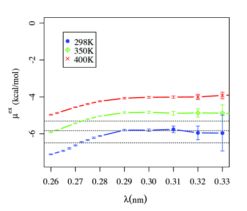
Figure 3: Dependence of the free energy $\mu^{\mathrm{ex}}$ predicted by the gaussian model on the conditioning radius $\lambda$. The horizontal dotted lines are the numerically exact results. The error bars indicate approximate 95% confidence intervals.

Table 1: Free energy contributions in kcal/mol associated with the gaussian model. The bottom value of the right-most column at each temperature gives the corresponding free energy evaluated by the histogram overlap method.

T(K)	$\lambda$ (nm)	$\mu^{\mathrm{ex}}_{\mathrm{HS}}\left(\lambda\right)$	$+kT\ln p\left(r\geq\lambda\right)$	$+\left\langle\varepsilon|r\geq\lambda\right\rangle$	$+\left\langle\delta\varepsilon^{2}|r\geq\lambda\right\rangle/2kT$	$=\mu^{\mathrm{ex}}$
298	0.2600	2.80	$-0.04$	$-19.74$	+9.87	= $-7.11\pm$ 0.02
	0.2650	2.99	$-0.13$	$-19.68$	+9.93	= $-6.89\pm$ 0.03
	0.2675	3.09	$-0.20$	$-19.59$	+9.97	= $-6.73\pm$ 0.04
	0.2700	3.19	$-0.31$	$-19.46$	+9.98	= $-6.60\pm$ 0.03
	0.2725	3.29	$-0.44$	$-19.27$	+9.97	= $-6.45\pm$ 0.03
	0.2750	3.40	$-0.60$	$-19.03$	+9.92	= $-6.31\pm$ 0.03
	0.2775	3.50	$-0.78$	$-18.73$	+9.83	= $-6.18\pm$ 0.04
	0.2800	3.61	$-0.98$	$-18.39$	+9.71	= $-6.05\pm$ 0.03
	0.2900	4.07	$-1.96$	$-16.75$	+8.89	= $-5.75\pm$ 0.04
	0.3000	4.56	$-3.09$	$-14.93$	+7.77	= $-5.69\pm$ 0.06
	0.3100	5.05	$-4.27$	$-13.21$	+6.67	= $-5.67\pm$ 0.18
	0.3200	5.61	$-5.45$	$-11.65$	+5.54	= $-5.95\pm$ 0.37
	0.3300	6.20	$-6.64$	$-10.30$	+4.78	= $-5.96\pm$ 0.97
						$-6.49$
350	0.2600	3.12	$-0.05$	$-18.43$	+9.44	= $-5.92\pm$ 0.02
	0.2625	3.23	$-0.09$	$-18.41$	+9.46	= $-5.81\pm$ 0.02
	0.2700	3.55	$-0.33$	$-18.14$	+9.47	= $-5.45\pm$ 0.02
	0.2750	3.77	$-0.62$	$-17.73$	+9.35	= $-5.23\pm$ 0.02
	0.2800	4.00	$-0.99$	$-17.15$	+9.10	= $-5.04\pm$ 0.01
	0.2900	4.50	$-1.92$	$-15.67$	+8.24	= $-4.85\pm$ 0.04
	0.3000	5.02	$-3.00$	$-14.05$	+7.20	= $-4.83\pm$ 0.06
	0.3100	5.58	$-4.13$	$-12.48$	+6.14	= $-4.89\pm$ 0.10
	0.3200	6.18	$-5.28$	$-11.01$	+5.24	= $-4.87\pm$ 0.22
	0.3300	6.80	$-6.41$	$-9.74$	+4.47	= $-4.88\pm$ 0.45
						$-5.83$
400	0.2600	3.30	$-0.06$	$-17.19$	+8.97	= $-4.98\pm$ 0.02
	0.2625	3.40	$-0.10$	$-17.16$	+8.99	= $-4.87\pm$ 0.03
	0.2700	3.74	$-0.35$	$-16.89$	+8.95	= $-4.55\pm$ 0.02
	0.2750	3.96	$-0.63$	$-16.49$	+8.80	= $-4.36\pm$ 0.03
	0.2800	4.20	$-0.98$	$-15.96$	+8.52	= $-4.22\pm$ 0.03
	0.2900	4.71	$-1.87$	$-14.60$	+7.69	= $-4.07\pm$ 0.05
	0.3000	5.25	$-2.89$	$-13.10$	+6.72	= $-4.02\pm$ 0.05
	0.3100	5.82	$-3.97$	$-11.64$	+5.78	= $-4.01\pm$ 0.06
	0.3200	6.42	$-5.06$	$-10.31$	+4.95	= $-4.00\pm$ 0.14
	0.3300	7.05	$-6.12$	$-9.12$	+4.27	= $-3.92\pm$ 0.18
						$-5.31$

The conditioning affects both the high-$\varepsilon$ and low-$\varepsilon$ tails of these distributions. The mean binding energy $\left\langle\varepsilon|r>\lambda\right\rangle$ increases with increasing $\lambda$ [Table 1], so we conclude that the conditioning eliminates atypical low-$\varepsilon$, well-bound configurations more than high-$\varepsilon$ configurations that reflect less favorable interactions. Nevertheless, because of the exponential weighting of the integrand of Eq. (1) and because the variances are large, the high-$\varepsilon$ side of the distributions is overwhelmingly the more significant in this free energy prediction.

Conversely, the fluctuation contribution exhibits a broad maximum for $\lambda<$ 0.29 nm, after which this contribution decreases steadily with increasing $\lambda$ [Table 1]. Evidently water molecules closest to the distinguished molecule, i.e., those closer than the principal maximum of oxygen-oxygen radial distribution function, don’t contribute importantly to the fluctuations. This is consistent with a quasi-chemical picture in which a water molecule and its nearest neighbors have a definite structural integrity.

The magnitude of the individual contributions to $\mu^{\mathrm{{ex}}}$ are of the same order as the net free energy; the mean binding energies are larger than that, as are the variance contributions in some cases. The variance contributions are about half as large as the mean binding energies, with opposite sign. It is remarkable and significant, therefore, that the net free energies at 298 K are within roughly 12% of the numerically exact value computed by the histogram-overlap method. The discrepancies at the higher temperatures are larger, and we will return to that point. A mean-field-like approximation that neglects fluctuations produces useless results.

We note that $p(r\geq\lambda)\approx$ 1 for the smallest values of $\lambda$ in Table 1. This leads to the awkward point that if $kT\ln{p(r\geq\lambda)}$ is zero, then the hard-sphere contribution $\mu^{\mathrm{{ex}}}_{\mathrm{{HS}}}$ is ill-defined. As a general matter, the sum $\mu^{\mathrm{{ex}}}_{\mathrm{{HS}}}+kT\ln{p(r\geq\lambda)}$ cannot be identified as a hard-sphere contribution. Since these terms have opposite signs, the net value can be zero or negative, and those possibilities are realized [Table 1]. To define the hard-sphere contribution more generally, we require $\mu^{\mathrm{{ex}}}_{\mathrm{{HS}}}$ to be continuous as $\lambda$ decreases, such that $p(r\geq\lambda)\rightarrow$ 1. All other terms of Eq.  (2) will be independent of $\lambda$ for values smaller than that, and we will require that of $\mu^{\mathrm{{ex}}}_{\mathrm{{HS}}}$ also.

From Fig. 3, we see that $\lambda>$ 0.30 nm clearly identifies a larger-size regime where the variation of the free energy with $\lambda$ is not statistically significant. Although we anticipate a decay toward the numerically exact value for $\lambda\rightarrow\infty$, the statistical errors become unmanageable for values of $\lambda$ much larger than 0.30 nm. When $\lambda$ = 0.30 nm a significant skew in $p(\varepsilon|r\geq\lambda)$ is not observed, as already noted with Fig. 2. The predicted free energy $\mu^{\mathrm{{ex}}}$ is then distinctly above the numerically exact value, suggesting that the gaussian model predicts too much weight in the high-$\varepsilon$ tail. We hypothesize that this sharper-than-gaussian tail behavior is due to the fact that a finite number of molecules make discrete contributions to the net $\varepsilon$ in this tail region. A model distribution exhibiting this distinction is

$$p\left(\varepsilon|r\geq\lambda\right)=\\ \left\{\prod\limits_{k=1}^{n}\int\pi\left(\varepsilon_{k}|r\geq\lambda\right)\right\}\delta\left(\varepsilon-\sum\limits_{k=1}^{n}\varepsilon_{k}\right)\mathrm{d}\varepsilon_{1}\ldots\mathrm{d}\varepsilon_{n}~{},$$ (3)

with $\pi\left(\varepsilon_{k}|r\geq\lambda\right)$ an elementary distribution with a sharp cut-off. The plug density

$$\pi\left(\varepsilon_{k}|r\geq\lambda\right)=\left(\frac{1}{\Delta\varepsilon}\right)H\left(\frac{\Delta\varepsilon}{2}-\left|\varepsilon_{k}-\frac{\left\langle\varepsilon|r\geq\lambda\right\rangle}{n}\right|\right),$$ (4)

with $H\left(x\right)$ the Heaviside function, is an example. This function is non-zero over an $\varepsilon$-width of

$$\Delta\varepsilon=\sqrt{12\left<\delta\varepsilon^{2}|r\geq\lambda\right>/n}$$ (5)

when the parameterization is set so that Eq. (3) is consistent with the previous notation. This leaves the number $n$ as a single further parameter; a larger $n$ indicates a larger range of gaussian behavior for $p(\varepsilon|r\geq\lambda)$. With the example Eq. (4) the evaluation of the thermodynamic result is elementary, and amounts to the replacement

$$\left<\delta\varepsilon^{2}|r\geq\lambda\right>\leftarrow\left<\delta\varepsilon^{2}|r\geq\lambda\right>\left(1-\frac{\beta^{2}\left<\delta\varepsilon^{2}|r\geq\lambda\right>}{10n}\right)$$ (6)

in Eq. (2) for large $n$.

Since we exploit a single further datum, a single parameter exhausts that information. When $\lambda$ = 0.30 nm, the values of $n$ that fit the numerically exact results are 21, 11, and 6 at $T$= 298, 350, and 400 K, respectively. These values are reasonable as indications of the discrete number of proximal water molecules that dominate solvent interactions with the distinguished molecule.

It is essential, however, to recognize that the sharper-than-gaussian hypothesis means sharper than the single gaussian of Eq. (2). A natural path for improvement of these results would be a multi-gaussian model, as was developed for careful evaluations of the electrostatic contribution to the free energy of liquid water Hummer et al. (1995, 1997). But some further points, which touch upon similarities of the multi-gaussian and quasi-chemical approaches, must be kept in mind. First, we are concerned here with contributions from a defined outer-shell region, the direct inner-shell contributions have been relegated to the $kT\ln p\left(r\geq\lambda\right)$ term of Eq. (2). Second, the multi-gaussian approach requires choosing a variable to stratify the distribution; in the quasi-chemical approach that variable is the number of occupants of the defined shell Pratt and Asthagiri (2006), presumably an inner outer-shell region here. Since this refinement has exhausted the data here, we don’t pursue those more refined approaches. But we also recognize that the initial model, Eq. (2), is a compact, simple implementation of quasi-chemical ideas.

The values of $n$ are found to correlate positively with the variance $\left<\delta\varepsilon^{2}|r\geq\lambda\right>$, such that $\Delta\varepsilon$ [Eq. (5)] is only weakly dependent on $\lambda$. At $T$ = 298 K, $\Delta\varepsilon\approx$ 2 kcal/mol, independent of $\lambda$. At the higher temperatures, $\Delta\varepsilon$ is 1-2 kcal/mol larger, and has a noticeable, linear dependence on $\lambda$. These empirical energy parameters are of reasonable magnitude by comparison with hydrogen-bond energies, and they do not correspond to weak interactions on a thermal scale.

Though these theoretical developments were unanticipated, it is possible to make some connection to classical theories. Assume that the $N$-molecule fluid can be satisfactorily described by a pair-decomposable potential energy function. Then a gaussian model for a joint distribution of binding energies $\varepsilon_{1}$ and $\varepsilon_{2}$, of molecules 1 and 2, respectively, predicts

$$\beta^{2}\left<\delta\varepsilon_{1}\delta\varepsilon_{2}|1,2\right>=\ln y\left(1,2\right)~{},$$ (7)

where $y\left(1,2\right)$ is the two-molecule indirect distribution function Hansen and McDonald (2006), and the average is conditional upon location of molecules at (1,2). A point of general interest is that Eq. (7) is a signature of the random-phase family of approximations, e.g. the Debye-Hückel theory. It is also interesting that Eq. (7) does not express a conventional mean-field contribution. However, if the molecules considered are significantly different, such a relation then is expected to resemble mean-field contributions of the classical type.

This work was carried out under the auspices of the National Nuclear Security Administration of the U.S. Department of Energy at Los Alamos National Laboratory under Contract No. DE-AC52-06NA25396. Financial support from the National Science Foundation (BES0518922) is gratefully acknowledged.

References

- Stillinger (1980) F. H. Stillinger, Science 209, 451 (1980).
- Widom (1967) B. Widom, Science 157, 375 (1967).
- Hummer et al. (1996) G. Hummer, S. Garde, A. E. García, A. Pohorille, and L. R. Pratt, Proc. Natl. Acad. Sci. USA 93, 8951 (1996).
- Ashbaugh and Pratt (2006) H. S. Ashbaugh and L. R. Pratt, Rev. Mod. Phys. 78, 159 (2006).
- Hummer et al. (2001) G. Hummer, J. C. Rasaiah, and J. P. Noworyta, Nature 414, 188 (2001).
- Rowlinson and Swinton (1982) J. S. Rowlinson and F. L. Swinton, Liquids and Liquid Mixtures (Butterworths, NY, 1982).
- Asthagiri et al. (2006) D. Asthagiri, H. S. Ashbaugh, A. Piryatinski, M. E. Paulaitis, and L. R. Pratt, Tech. Rep., Los Alamos Natl. Lab. LA-UR-06-3812 (2006).
- Asthagiri et al. (2003) D. Asthagiri, L. R. Pratt, and J. D. Kress, Phys. Rev. 68, 041505 (2003).
- Paliwal et al. (2006) A. Paliwal, D. Asthagiri, L. R. Pratt, H. S. Ashbaugh, and M. E. Paulaitis, J. Chem. Phys. 124 (2006).
- Paulaitis and Pratt (2002) M. E. Paulaitis and L. R. Pratt, Adv. Prot. Chem. 62, 283 (2002).
- Beck et al. (2006) T. L. Beck, M. E. Paulaitis, and L. R. Pratt, The potential distribution theorem and models of molecular solutions (Cambridge University Press, 2006).
- Hummer et al. (1995) G. Hummer, L. R. Pratt, and A. E. García, J. Phys. Chem. 99, 14188 (1995).
- Hummer et al. (1997) G. Hummer, L. R. Pratt, and A. E. García, J. Am. Chem. Soc. 119, 8523 (1997).
- Pratt and Asthagiri (2006) L. R. Pratt and D. Asthagiri, in Free Energy Calculations. Theory and Applications in Chemistry and Biology, edited by C. Chipot and A. Pohorille (Springer, Berlin, 2006), chap. 9. Potential distribution methods and free energy models of molecular solutions.
- Hansen and McDonald (2006) J.-P. Hansen and I. R. McDonald, Theory of simple liquids (Elsevier, 2006).