Abstract

The inequality is computed through the so-called Gini index. The population is assumed to have the variable of interest distributed according to the Gamma probability distribution. The results show that the Gini index is reduced when the population is grouped. The number of individuals in the groups is the relevant parameter, but this number does not need to be very large in order to obtain a very substantial reduction of inequality.

PACS:

87.23.Ge Dynamics of social systems

02.50.-r Probability theory, stochastic processes, and statistics

65.50.+m Thermodynamic properties and entropy

Keywords: econophysics, thermodynamics, probability distributions, Gini index, inequality, entropy

1. INTRODUCTION

The Gamma probability distribution is a powerful and flexible distribution that applies with absolute precision to a great variety of problems and systems in thermodynamics, solid state physics, economics, etc.

The present author has suggested [9] that this distribution should replace, in particular, the Planck distributions, used to describe the blackbody radiation distribution, as well as the Maxwell velocity distribution for ideal gases.

Also, in the area of econophysics, the Gamma distribution should replace profitably all of the other distributions currently used, such as the following (some of them are the same one and are instances of the Gamma distribution): Gibbs, negative exponential or simply exponential, Boltzmann, log-normal, power law, Pareto-Zipf, Erlang and Chi-squared. Simulations and applications using the Gamma distribution [1], [7], [8], [10], have shown that the Gamma distribution better fits the actual distribution of the variable of interest.

In the present paper the author develops the formula to compute the Gini index corresponding to some variable distributed in a population according to the Gamma probability distribution.

2. THE GINI INDEX

The Gini index, Gini ratio or Gini coefficient, is probably the most well-known and broadly used measure of inequality used in economic literature.

The Gini index derives from the Lorenz Curve. To plot a Lorenz curve, order the observations from lowest to highest on the variable of interest, such as income, and then plot the cumulative proportion of the population on the X-axis and the cumulative proportion of the variable of interest on the Y-axis.

If all individuals have the same income the Lorenz curve is a straight diagonal line, called the line of equality. If there is any inequality, then the Lorenz curve falls below the line of equality. The total amount of inequality can be summarized by the Gini index, which is the proportion of the area enclosed by the lines of equality and the Lorenz curve divided by the total triangular area under the line of equality.

In the figure below, the diagonal line represents perfect equality. The greater the deviation of the Lorenz curve from this line, the greater the inequality. The Gini index is double the area between the equality diagonal and the Lorenz curve. The minimum value of the Gini can be zero (perfect equality) and the greater can be one (the case when a single member of the population holds all of the variable). [4]

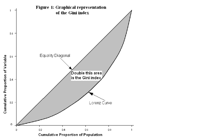
Figure 1: The Gini index

3. THE GAMMA DISTRIBUTION

The author of this paper has proposed [9] that the Gamma distribution seems to be the correct distribution of blackbody energy radiation, money and other variables from comparable continuous systems.

The Gamma probability distribution function (pdf) [9] has the form

$$P(p,\lambda,x)=\frac{\lambda^{p}\cdot x^{p-1}}{Exp(\lambda\cdot x)\cdot\Gamma(p)}$$ (1)

The parameters of this distribution are called the shape parameter (p) and the scale parameter ($\lambda$).

The Gamma function satisfies:

$$\Gamma(p)=\int\nolimits_{0}^{\infty}x^{p-1}e^{-x}dx$$ (2)

This expression is the equivalent, for the Gamma distribution, of the partition function defined in classical thermodynamics for the Boltzmann distribution.

The incomplete Gamma function $\Gamma(p,\lambda\cdot x)$, used in the following, has a similar integrand, and the only difference is that the lower limit of integration is $\lambda\cdot x$ instead of zero.

If the value of the variable p is particularized to an integer value then this distribution converts into the Erlang distribution.

If the variable p has the value 1, the Gamma distribution converts into the negative exponential distribution, also called Boltzmann, Gibbs, Boltzmann-Gibbs or simply exponential law.

In the area of econophysics, the use of the so-called Pareto or power law distribution is very common, although it is obvious that it is not a probability distribution (where the sum or integral of probabilities is equal to the unity) because its integral does not converge. It should be profitably replaced by the Gamma distribution with the proper parameters.

The average of a quantity x distributed according to the Gamma distribution is

$$\left\langle x\right\rangle=\frac{p}{\lambda}$$ (3)

As a result, if we keep the average of x equal to the unity then p must
be equal to $\lambda$. Nevertheless the larger the values of $p=\lambda$ the smaller the variance since this is given by:

$$\sigma^{2}=\frac{p}{\lambda^{2}}$$ (4)

The maximum of the Gamma distribution is at the position

$$x_{\max}=\frac{p-1}{\lambda}=\left\langle x\right\rangle-\frac{1}{\lambda}$$ (5)

4. INCOME OF GROUPS OF EARNERS

Dragulescu and Yakovenko [2] compute the distribution of the combined income of two earners and get the following formula, which they find in excellent agreement with the income data of the USA population. They assume that the income r of two earners is the sum of the individual incomes: r=r1+r2. Hence, the total income pdf, $P_{2}(r)$, is given by the convolution

$$P_{2}(r)=\int\nolimits_{0}^{r}P_{1}(x)\cdot P_{1}(r-x)dx=\frac{r}{R^{2}}e^{-r/R}$$ (6)

where the individual incomes r1 and r2 are assumed to be uncorrelated and to have exponential distributions of the form: P₁(r)=e^-r/R/R, where R is the average income of the population.

As is well known, the exponential distribution, also called Boltzmann or Gibbs distribution, is a special case of the Gamma distribution when the parameter p is equal to 1. Whereas the resulting expression (6) is a Gamma distribution with parameter p=2. This expression describes the income distribution of a population of groups of two earners.

By generalizing this idea and maintaining constant the scale parameter $\lambda$ we can verify that the convolution of two Gamma distributions, with respective shape parameters p1 and p2, produces another Gamma distribution with shape parameter p1+p2:

$$P(p1+p2,\lambda,r)=\int\nolimits_{0}^{r}P(p1,\lambda,x)\cdot P(p2,\lambda,r-x)dx$$

$$P(p1+p2,\lambda,r)=\frac{\lambda^{p1+p2}}{\Gamma(p1+p2)}r^{p1+p2-1}e^{-\lambda\cdot r}$$ (7)

If we interpret the shape parameter p as the number of earners then equation (7) simply says that the income distribution of the sum of incomes of two groups, with respective number of earners p1 and p2, is given by the (Gamma) income distribution of the sum of earners. The parameters p can have any positive real values.

5. THE GINI INDEX OF GROUPED EARNERS

The horizontal axis of the Lorenz curve, x(r), represents the cumulative fraction of population with income below r, and the vertical axis y(r) represents the fraction of income this population accounts for.
The respective values for these fractions are given by the following formulas [3]:

$$x(r)=\int\nolimits_{0}^{r}P(p,\lambda,r^{\prime})dr^{\prime}=1-\frac{\Gamma(p,\lambda\cdot r)}{\Gamma(p)}$$ (8)

$$y(r)=\frac{\int\nolimits_{0}^{r}r^{\prime}\cdot P(p,\lambda,r^{\prime})dr^{\prime}}{\int\nolimits_{0}^{\infty}r^{\prime}\cdot P(p,\lambda,r^{\prime})dr^{\prime}}=1-\frac{\Gamma(p+1,\lambda\cdot r)}{\Gamma(p+1)}$$ (9)

The range of these variables is between 0 and 1. The Gini index for the Gamma probability distribution is obtained replacing (8) and (9) into the following integral:

$$G=2\cdot\int\nolimits_{0}^{1}(x-y)\cdot dx$$ (10)

or, as a function of r:

$$G=1-2\cdot\int\nolimits_{0}^{\infty}y(r)\frac{dx(r)}{dr}\cdot dr$$ (11)

Whose result is:

$$G=\frac{\Gamma(2p+1)}{4^{p}\cdot\Gamma(p+1)^{2}}$$ (12)

This shows that the gini index is independent of the values of $\lambda$ but depends on the number of individuals in the groups, p. For example, if we instantiate the parameter p to 1, this formula gives the Gini index for the exponential distribution, which is 1/2. This is the Gini for one earner and for any value of the parameter $\lambda$.

Let us compute the Gini for the Gamma distribution for a few earners (integer values of the parameter p).

The following table shows the Gini index corresponding to each value of p between 1 and 5, and the proportion of the first Gini relative to the second, etc.

p	Gini(p)	Proportion
		Gini(p)/Gini(p+1)
1	1/2 = 0.500	1.33
2	3/8 = 0.375	1.20
3	5/16 = 0.3125	1.14
4	35/128 = 0.2734	1.11
5	63/256 = 0.2461

Table1. Gini index as a function of the number of earners (p)

This table shows an important reduction of the Gini index, of 0.125 points when the number of earners in the groups passes from 1 to 2 and of an additional 0.0625 when the number of earners rises from 2 to 3. The proportion between the Gini index corresponding to a given number p of earners and the following, p+1, tends to 1 as the number of earners in the groups grows.

The following simple, but approximate, formula provides values up to around 11.4% lower than the previous exact formula:

$$G=\frac{1}{2\cdot\sqrt{p}}$$

For example for p=4, this formula gives the value 0.25, whereas the exact value, shown in the previous table, is around 0.2734; for p=100 this formula provides 0.05, but the exact value is close to 0.05635.

It is important to know this mechanism for the reduction of inequality. But, of course, the next more important issue would be how to form the groups and achieve the redistribution, of the individual income of each one of the individuals that constitute the group of earners, among all of them. This point is addressed very briefly here and should be addressed more deeply by other investigators.

The persons that constitute the groups must be selected randomly from the entire population, which is assumed to have a Gamma probability distribution of the income. Otherwise I would prefer to “share my wealth” with Gates and Rockefellers.

More seriously, the financial institutions, welfare, non-governmental organizations, etc. should prefer to finance and help groups instead of to particular individuals. There already are many forms of organizations in the world that procure this kind of behavior, such as cooperatives, kibbutz, comunas (from common), families, etc., which have demonstrated to be a very good mechanism for the redistribution of the income and consequent reduction of poverty and inequality.

6. ENTROPY OF THE GAMMA DISTRIBUTION

The entropy of the Gamma distribution was defined by the present author in other paper [9] in the form:

$$S(p,\lambda,x)=1-\frac{\Gamma(p,\lambda\cdot x)}{\Gamma(p)}$$ (13)

where p and $\lambda$ are the shape and scale parameters of the Gamma distribution and x is the variable being distributed. Note that this expression is identical to (8).

Expression (13) is the definition of the “non-extensive” entropy, in the sense that it does not have units and is precisely the cumulative distribution function (CDF) of the Gamma probability distribution. The incomplete Gamma function alone, which is the numerator in this expression, can be considered as the corresponding “extensive entropy”.

Litchfield [5] compares several measures of inequality and exposes, following Cowell, that any member of the Generalized Entropy (GE) class of inequality measures satisfies five axioms, which we now try to apply to the Gamma entropy:

The Pigou-Dalton Transfer Principle. An income transfer from a poorer person to a richer person should register as a rise (or at least not as a fall) in inequality and an income transfer from a richer to a poorer person should register as a fall (or at least not as an increase) in inequality.

This axiom does not apply, since the Gamma distribution is obtained from an equilibrium equation among actors with different incomes. Any transfer between them should maintain the Gamma distribution and hence also the equilibrium. The entropy of the Gamma distribution does not depend on the individual incomes but on the complete statistical distribution.

Income Scale Independence. This requires that the inequality measure be invariant to changes in scale as happens say when changing currency unit.

The Gamma distribution passes this test because the parameter $\lambda$ works as an average that suppresses any additional factor in the variable x.

Principle of Population. This principle requires inequality measures to be invariant to replications of the population: merging two identical distributions should not alter inequality.

Again, the Gamma distribution is a statistical distribution and therefore is not affected by the number of individuals in the population.

Anonymity. This axiom, sometimes also referred to as ‘Symmetry’, requires that the inequality measure be independent of any characteristic of individuals other than their income.

The Gamma distribution satisfies this axiom trivially.

Decomposability. This requires overall inequality to be related consistently to constituent parts of the distribution, such as population sub-groups. For example if inequality is seen to rise amongst each sub-group of the population then we would expect inequality overall to also increase.

The Gamma distribution satisfies this axiom through the Gini index associated with the Gamma distribution, as was proved in section 5. The parameter p of the Gamma entropy also takes into account the number of members in the groups, but with a more compact expression.

7. CONCLUSIONS

The analysis shown in section 4 proves that the Gamma entropy solves the so-called Gibbs’ paradox. Current Physics assumes that the entropy should not change as a result of mixing two amounts of identical gases. In the present paper it has been proved that this assumption does not hold when we use non-extensive definitions of entropy, such as the cumulative or normalized Gamma entropy. It is also doubtful that the entropy will not change for the extensive case.

For example, in his “Thermodynamics Lecture Notes” [6], Prof. Professor Donald B. Melrose, Director, RCfTA and Head of Theoretical Physics, School of Physics, University of Sydney says: “It follows that the entropy increases in this case and it is not difficult to see that the entropy change as a result [of] mixing is always positive. If they [the gases] are identical then the change in entropy must be zero and yet the calculation seems to imply that there is a change in entropy. This is referred to as the Gibbs paradox. There is no simple physical resolution of the Gibbs paradox within the framework of classical statistical mechanics.”

It is clear that the entropy associated with the distribution (7), which is the distribution of the combined income of two earners, is given by the Gamma entropy with parameter (p1+p2), whereas the income distributions of each one of the earners have associated individual Gamma entropies with respective parameters p1 and p2. Therefore, the entropy associated with the sum of a certain variable belonging to two or more actors must change even though the actors were identical. The original entropies are recovered if, for the studied variable, the individual incomes of the actors are again considered independently.

In both cases the population is the same but the values for the studied variable are different. The different income values depend on the grouping of individuals and on the corresponding averaging of the variable.

The non-extensive entropy computed for groups with the same number of individuals must not change for a new population obtained combining two populations that have the same statistical properties. The statistical (non-extensive) properties of the combined population, such as average temperature, are conserved; however, the corresponding extensive properties, such as the total energy or money of the system and even the particular values corresponding to each particle or individual of the population, necessarily change.

References

- [1] Bhattacharya, Mukherjee & Manna. Detailed simulation results for some wealth distribution models in Econophysics. arXiv: physics/0504161 v1, Apr 2005.
- [2] Dragulescu, Adrian &Yakovenko, Victor. Statistical Mechanics of Money, Income, and Wealth: A Short Survey. arXiv: cond-mat/0211175. Nov. 2002.
- [3] Dragulescu, Adrian. Applications Of Physics To Economics And Finance: Money, Income, Wealth, And The Stock Market. arXiv: cond-mat/0307341 v2, 16 Jul. 2003.
-
[4]
Hale, Travis. The Theoretical Basics of Popular Inequality
Measures. University of Texas Inequality Project.
http://utip.gov.utexas.edu/tutorials/theo_basic_ineq_measures.doc -
[5]
Litchfield, Julie A. Inequality: Methods and Tools. March
1999.
http://www.worldbank.org/poverty -
[6]
Melrose, Donald B. Lecture 2: Maxwell Distribution: Ideal
Gases. http://ckw.phys.ncku.edu.tw/public/pub/WebSources/Melrose/
www.physics.usyd.edu.au/rcfta/thermo.html - [7] Patriarca, Chakraborti & Kaski. Gibbs versus non-Gibbs distributions in money dynamics. Physica A 340 (2004) 334-339. Elsevier.
- [8] Patriarca, Chakraborti & Germano. Influence of saving propensity on the power law tail of wealth distribution. arXiv: physics/0506028 v1, Jun 2005.
- [9] Saá, Diego. On An Improvement Of The Planck Radiation Energy Distribution. In: http://arxiv.org/abs/physics/0603117 v3, Jul 2006.
- [10] Scafetta, Picozzi & West. A trade-investment model for distribution of wealth. Physica D 193 (2004) 338-352. Elsevier.