Evolution of surface gravity waves over a submarine canyon

Abstract

The effects of a submarine canyon on the propagation of ocean surface waves are examined with a three-dimensional coupled-mode model for wave propagation over steep topography. Whereas the classical geometrical optics approximation predicts an abrupt transition from complete transmission at small incidence angles to no transmission at large angles, the full model predicts a more gradual transition with partial reflection/transmission that is sensitive to the canyon geometry and controlled by evanescent modes for small incidence angles and relatively short waves. Model results for large incidence angles are compared with data from directional wave buoys deployed around the rim and over Scripps Canyon, near San Diego, California, during the Nearshore Canyon Experiment (NCEX). Wave heights are observed to decay across the canyon by about a factor 5 over a distance shorter than a wavelength. Yet, a spectral refraction model predicts an even larger reduction by about a factor 10, because low frequency components cannot cross the canyon in the geometrical optics approximation. The coupled-mode model yields accurate results over and behind the canyon. These results show that although most of the wave energy is refractively trapped on the offshore rim of the canyon, a small fraction of the wave energy ‘tunnels’ across the canyon. Simplifications of the model that reduce it to the standard and modified mild slope equations also yield good results, indicating that evanescent modes and high order bottom slope effects are of minor importance for the energy transformation of waves propagating across depth contours at large oblique angles.

MAGNE ET AL. Waves over submarine canyons Fabrice Ardhuin, Centre Militaire d’Océanographie, Service Hydrographique et Océanographique de la Marine, 29609 Brest, France. (ardhuin@shom.fr) Gindraft=false

1 Introduction

Waves are strongly influenced by the bathymetry when they reach shallow water areas. Munk and Traylor [1947] conducted a first quantitative study of the effects of bottom topography on wave energy transformation over Scripps and La Jolla Canyons, near San Diego, California. Wave refraction diagrams were constructed using a manual method, and compared to visual observations. Fairly good agreement was found between predicted and observed wave heights. Other effects such as diffraction were found to be important elsewhere, for sharp bathymetric features (e.g. harbour structures or coral reefs), prompting Berkhoff [1972] to introduce an equation that represents both refraction and diffraction. Berkhoff’s equation is based on a vertical integration of Laplace’s equation and is valid in the limit of small bottom slopes. It is widely known as the mild slope equation (MSE). A parabolic approximation of this equation was proposed by Radder [1979], and further refined by Kirby [1986] and [Dalrymple and Kirby(1988)].

O’Reilly and Guza [1991, 1993] compared Kirby’s [1986] refraction-diffraction model to a spectral geometrical optics refraction model based on the theory of Longuet-Higgins [1957]. The two models generally agreed in simulations of realistic swell propagation in the Southern California Bight. However, both models assume a gently sloping bottom, and their limitations in regions with steep topography are not well understood. Booij [1983], showed that the MSE is valid for bottom slopes as large as $1/3$ for normal wave incidence. To extend its application to steeper slopes, Massel [1993 ; see also Chamberlain and Porter, 1995] modified the MSE by including terms of second order in the bottom slope, that were neglected by Berkhoff [1972]. This modified mild slope equation (MMSE) includes terms proportional to the bottom curvature and the square of the bottom slope. Chandrasekera and Cheung [1997] observed that the curvature terms significantly change the wave height behind a shoal, whereas the slope-squared terms have a weaker influence. Lee and Yoon [2004] noted that the higher order bottom slope terms change the wavelength, which in turn affects the refraction. In spite of these improvements, an important restriction of these equations is that the vertical structure of the wave field is described by the Airy solution of waves over a horizontal bottom. Hence the MMSE cannot describe the wave field accurately over steep bottom topography. Thus, Massel [1993] introduced an additional infinite series of local modes (’evanescent modes’ or ’decaying waves’), that allows a local adaptation of the wave field [see also Porter and Staziker, 1995], and converges to the exact solution of Laplace’s equation, except at the bottom interface. Indeed, the vertical velocity at the bottom is still zero, and is discontinuous in the limit of an infinite number of modes. Recently, Athanassoulis and Belibassakis [1999] added a ’sloping bottom mode’ to the local mode series expansion, which properly satisfies the Neuman bottom boundary condition. This approach was further explored by Chandrasekera and Cheung, [2001] and Kim and Bai, [2004]. Although the sloping-bottom mode yields only small corrections for the wave height, it significantly improves the accuracy of the velocity field close to the bottom. Moreover, this mode enables a faster convergence of the series of evanescent modes, by making the convergence mathematically uniform.

As these steep topography models are becoming available, one may wonder if this level of sophistication is necessary to accurately describe the transformation of ocean waves over natural continental shelf topography. It is expected that if such models are to be useful anywhere, it should be around steep submarine canyons. Surprisingly, a geometrical optics refraction model that assumes weak amplitude gradients on the scale of the wavelength, usually corresponding to gentle bottom slopes, was found to yield accurate predictions of swell transformation over Scripps canyon [Peak, 2004]. The practical limitations of mild slope approximations for natural seafloor topography are clearly not well established.

The goal of the present paper is to understand the propagation of waves over a submarine canyon, including the practical imitations of geometrical optics theory for the associated large bottom slopes. Numerical models will be used to sort out the relative importance of refraction, and diffraction effects. Observations of ocean swell transformation over Scripps and La Jolla Canyons, collected during the Nearshore Canyon Experiment (NCEX), are compared with predictions of the three-dimensional (3D) coupled-mode model. This model is called NTUA5 because its present implementation will be limited to a total of 5 modes [Belibassakis et al., 2001]. This is the first verification of a NTUA-type model with field observations, as previous model validations were done with laboratory data. This application of NTUA5 to submarine canyons is not straightforward since the model is based on the extension of the two-dimensional (2D) model of [Athanassoulis and Belibassakis(1999)], and requires special care in the position of the offshore boundary and the numerical damping of scattered waves along the boundary. Further details on these and software developments, and a comparison with results of the SWAN model [Booij et al., 1999] for the same NCEX case are given by [Gerosthathis et al.(2005)Gerosthathis, Belibassakis, and Athanassoulis].

Here, model results are compared with two earlier models which assume a gently sloping bottom. These are the parabolic refraction/diffraction model REF/DIF1 (V2.5) [Kirby, 1986], applied in a spectral sense, and a spectral refraction model based on backward ray tracing [Dobson, 1967 ; O’Reilly and Guza, 1993]. A brief description of the coupled-mode model and the problems posed by its implementation in the NCEX area is given in section 2. Although our objective is the understanding of complex 3D bottom topography effects in the NCEX observations, this requires some prior analysis, performed in section 3, of reflection and refraction patterns over idealized 2D canyons. Results are presented for realistic transverse canyon profiles, including a comparison with the 2D analysis of infragravity wave observations reported by [Thomson et al.(2005)Thomson, Elgar, and Herbers]. Comparisons of 3D models with field data are presented in section 4 for representative swell events observed during NCEX. Conclusions follow in section 5.

2 Numerical Models

The fully elliptic 3D model developed by Belibassakis et al. [2001] is based on the 2D model of Athanassoulis and Belibassakis [1999]. These authors formulate the problem as a transmission problem in a finite subdomain of variable depth $h_{2}(x)$ (uniform in the lateral y-direction), closed by the appropriate matching conditions at the offshore and inshore boundaries. The offshore and inshore areas are considered as incidence and transmission regions respectively, with uniform but different depths ($h_{1}$, $h_{3}$), where complex wave potential amplitudes $\varphi_{1}$ and $\varphi_{3}$ are represented by complete normal-mode series containing the propagating and evanescent modes.

The wave potential $\varphi_{2}$ associated with $h_{2}$ (region $2$), is given by the following local mode series expansion:

$$\varphi_{2}(x,z) = \varphi_{-1}(x)Z_{-1}(z;x)+\varphi_{0}(x)Z_{0}(z;x)$$ (1)

$$+\sum_{n=1}^{\infty}\varphi_{n}(x)Z_{n}(z;x),$$

where $\varphi_{0}(x)Z_{0}(z;x)$ is the propagating mode and $\varphi_{n}(x)Z_{n}(z;x)$ are the evanescent modes. The additional term $\varphi_{-1}(x)Z_{-1}(z;x)$ is the sloping-bottom mode, which permits the consistent satisfaction of the bottom boundary condition on a sloping bottom. The modes allow for the local adaptation of the wave potential. The functions $Z_{n}(z;x)$ which represent the vertical structure of the $n^{\mathrm{th}}$ mode are given by,

$$Z_{0}(z,x)=\frac{\cosh[k_{0}(x)(z+h(x))]}{\cosh(k_{0}(x)h(x))},$$ (2)

$$Z_{n}(z,x)=\frac{\cos[k_{n}(x)(z+h(x))]}{\cos(k_{n}(x)h(x))},~{}~{}~{}n=1,2,...,$$ (3)

$$Z_{-1}(z,x)=h(x)\left[\left(\frac{z}{h(x)}\right)^{3}+\left(\frac{z}{h(x)}\right)^{2}\right],$$ (4)

where $k_{0}$ and $k_{n}$ are the wavenumbers obtained from the dispersion relation (for propagating and evanescent modes), evaluated for the local depth $h=h(x)$:

$$\omega^{2}=gk_{0}\tanh{k_{0}h}=-gk_{n}\tan{k_{n}h},$$ (5)

with $\omega$ the angular frequency

As discussed in Athanassoulis and Belibassakis [1999], alternative formulations of $Z_{-1}$ exist, and the extra sloping-bottom mode controls only the rate of convergence of the expansion (1) to a solution that is indeed unique. The modal amplitudes $\varphi_{n}$ are obtained by a variational principle, equivalent to the combination of Laplace’s equation, the bottom and surface boundary conditions, and the matching conditions at the side boundaries, leading to the coupled-mode system,

$$\sum_{n=-1}^{\infty}a_{mn}(x)\varphi^{\prime\prime}_{n}(x) + b_{mn}(x)\varphi^{\prime}_{n}(x)+c_{mn}(x)\varphi_{n}(x)=0,$$ (6)

$$\mathrm{for}\quad(m=-1,0,1,...)$$

where $a_{mn}$, $b_{mn}$ and $c_{mn}$ are defined in terms of the $Z_{n}$ functions, and the appropriate end-conditions for the mode amplitudes $\varphi_{n}$ ; for further details, see see Athanassoulis and Belibassakis [1999]. The sloping-bottom mode ensures absolute and uniform convergence of the modal series. The rate of decay for the modal function amplitude is proportional to ($n^{-4}$). Here, the number of evanescent modes is truncated at $n=3$, which ensures satisfactory convergence, even for bottom slopes exceeding 1.

This 2D solution is further extended to realistic 3D bottom topographies by Belibassakis et al. [2001]. In 3D, the depth $h_{2}$ is decomposed into a background parallel-contour surface $h_{i}(x)$ and a scattering topography $h_{d}(x,y)$. The 3D solution is then obtained as the linear superposition of appropriate harmonic functions corresponding to these two topographies. There is no limitation on the shape and amplitude of the bottom represented by $h_{d}(x,y)$ except that $h_{d}>0$, which can always be enforced by a proper choice of $h_{i}$, for further details see Belibassakis et al. [1999]. The wave potential solution over the 2D topography ($h_{i}$) is governed by the equations described previously. The wave potential associated with the scatterers ($h_{d}$) is obtained as the solution of a 3D scattering problem. The decomposition of the topography in $h_{d}$ and $h_{i}$ is not uniquely defined by the constraints that $h_{i}$ is invariant along $y$ and $h_{d}>0$, and there is thus no simple physical interpretation of the scattered field which corresponds to both reflection and refraction effects. The main benefit of this decomposition is that the scattered wave field propagates out of the model domain along the entire boundary, which greatly simplifies the specification of the horizontal boundary conditions.

In practice we chose

$$h_{i}(x)=\min\left\{h(x,y)\quad\mathrm{for}\quad y\in\left[y_{\mathrm{min}},y_{\mathrm{max}}\right]\right\}.$$ (7)

Further, the bathymetry $h_{i}+h_{d}$ is modified by including a transition region for $y<y_{\mathrm{min}}$ and $y>y_{\mathrm{max}}$ in which $h_{d}$ goes to zero at the model boundary, so that no scattering sources are on the boundary and waves actually propagate out of the domain. This modification of the bathymetry does not change the propagation of the incoming waves, provided that the offshore boundary is in uniform water depth, as in the cases described by [Belibassakis et al.(2001)Belibassakis, Athanassoulis, and Gerostathis], or in deep enough water so that a uniform water depth can be prescribed without having an effect on the waves. Solutions are obtained by solving a coupled-mode system, similar to Eq.(6), but extended to two horizontal dimensions $(x,y)$, and coupled with the boundary conditions ensuring outgoing radiation. The spatial grid for the scattered field is extended with a damping layer all around the boundary [Belibassakis et al., 2001].

Both $2$D and $3$D implementations of this NTUA5 model are used here to investigate wave propagation over a submarine canyon. If we neglect the sloping-bottom mode and the evanescent modes, and retain in the local-mode series only the propagating mode $\varphi_{0}(x,y)$, this model (NTUA5) exactly reduces to MMSE [e.g. Chandrasekara and Cheung, 1997],

$$\nabla^{2}\varphi_{0}(x,y) + \frac{\nabla(CC_{g})}{CC_{g}}{\mathbf{\cdot}}\nabla\varphi_{0}(x,y)$$ (8)

$$+ \left[k_{0}^{2}+f_{1}\nabla^{2}h+f_{2}(\nabla h)^{2}\right]\varphi_{0}(x,y)=0,$$

where $f_{1}=f_{1}(x,y)$ and $f_{2}=f_{2}(x,y)$ are respectively functions dependent on the bottom curvature and slope-squared terms. From Eq.(8), the MSE is obtained by further neglecting the curvature and slope-squared terms.

In the following sections, these two formulations (MSE and MMSE) will be compared to the full 5-mode model to examine the importance of steep bottom slope effects, which are fully accounted for in this model. The MSE and MMSE solutions are obtained by exactly the same scattering method described above with the same computer code in which the high order bottom slope terms and/or evanescent modes are turned off. For 3D calculations, our use of a regular grid sets important constraints on the model implementation due to the requirements to have the offshore boundary in deep water and sufficient resolution to resolve the wavelength of waves in the shallowest parts of the model domain. These constraints put practical limits on the domain size for a given wave period and range of water depths. Here a minimum of 7 points per wavelength in 10 m depth was enforced, in a domain that extends 4–6 km offshore. Such a large domain with a high resolution leads to memory intensive inversion of large sparse matrices. However, the NTUA, MSE and MMSE models are linear, and thus the propagation of the different offshore wave components can be performed separately, sequentially or in parallel.

Before considering the full complexity of the 3D Scripps-La Jolla Canyon system, we first examine the behavior of these models in the case of monochromatic waves propagating over $2$D idealized canyon profiles (transverse sections of the actual canyons). We consider both the relatively wide La Jolla Canyon where infragravity wave reflection was reported recently [Thomson et al. 2005], and the narrow Scripps Canyon, that was the focus of the NCEX swell propagation study.

3 Idealized 2D canyon profiles

3.1 Transverse section of La Jolla Canyon

We investigate monochromatic waves propagating at normal incidence over a transverse section of the La Jolla Canyon (Figures 1,2), which is relatively deep (120 m) and wide (350 m). Oblique incidence will not be considered for this canyon because the results are similar to those obtained for Scripps Canyon (discussed below).

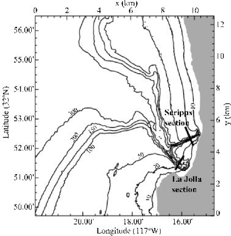
Figure 1: Bathymetry around La Jolla and Scripps canyons, and definition of transverse sections for idealized calculations.

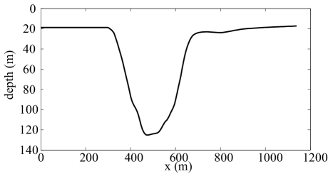
Figure 2: Water depth across the La Jolla canyon section.

Reflection coefficients $R$ for the wave amplitude are computed using the MSE, the MMSE, and the full coupled-mode model NTUA5. $R$ is easily obtained using the natural decomposition provided by the scattering method, and is defined as the ratio between the scattered wave potential amplitude, up-wave of the topography, and the amplitude of the imposed propagating wave. In addition, a stepwise bottom approximation model developed by Rey [1992], based on the matching of integral quantities at the boundaries of adjacent steps, is used to evaluate $R$ [see Takano, 1960; Miles, 1967; Kirby and Dalrymple, 1983]. This model is known to converge to the exact value of $R$, and will be used as a benchmark for this study.

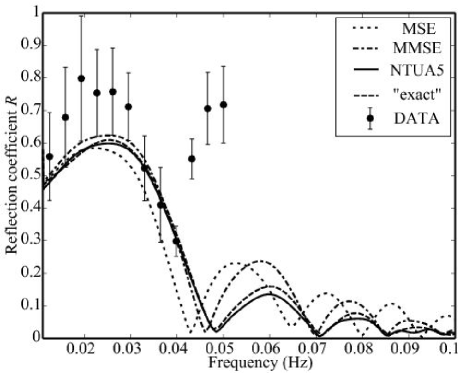
Figure 3: Amplitude reflection coefficient $R$ for waves propagating at normal incidence over the La Jolla canyon section (figure 2) using several numerical models, and observed infragravity reflections for near-normal incidence angles [Thomson et al., 2005]

.

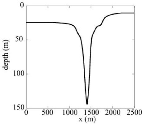
Figure 4: Water depth across the Scripps canyon section.

The canyon profile is resolved with 70 steps which was found to be sufficient to obtain a converging result. The predicted values of $R$ as a function of wave frequency $f$ (Figure 3), are characterized by maxima and minima, which are similar to the rectangular step response shown in Mei and Black [1969], Kirby and Dalrymple [1983a], and Rey et al. [1992]. The spacing between the minima or maxima is defined by the width of the step or trench, which imposes resonance conditions, leading to constructive or destructive interferences. Both the MSE and MMSE models are found to generally overestimate the reflection at high frequencies, whereas the NTUA5 model is in good agreement with the benchmark solution. The sloping-bottom mode included in NTUA5 has a negligible impact on the wave reflection in this and other cases discussed below. The only other difference between the NTUA5 and the MMSE models is the addition of the evanescent modes which, through their effect on the near wave field solution modify significantly the far field, including the overall reflection and transmission over the canyon.

[Thomson et al.(2005)Thomson, Elgar, and Herbers] investigated the transmission of infra-gravity waves with frequencies in the range $0.006$–$0.05$ Hz across this same canyon. Based on pressure and velocity time series at two points located approximately at the ends of the La Jolla section these authors estimated energy reflection coefficients as a function of frequency. In a case of near-normal incidence they observed a minimum of wave reflection at about 0.04 Hz, generally consistent with the present results (figure 3). [Thomson et al.(2005)Thomson, Elgar, and Herbers] further found a good fit of their observations to the theoretical reflection across a rectangular trench as given by [Kirby and Dalrymple(1983)] in the limit of long waves, and neglecting evanescent modes. This approximation is appropriate for the long infragravity band for which the effects of evanescent modes are relatively weak. The observations of [Thomson et al.(2005)Thomson, Elgar, and Herbers] also agree well with the various models applied here to the actual canyon profile (figure 3). At higher swell frequencies ($f>0.05$ Hz), the MSE, MMSE and NTUA model results diverge for normal incidence (figure 3). However, contrary to the beach-generated infragravity waves, swell arrives from the open ocean and thus always reaches this canyon with a large oblique angle, for which the differences between these models are small (not shown).

3.2 Transverse section of Scripps Canyon

3.2.1 Normal incidence

The north branch of the canyon system, Scripps Canyon, provides a very different effect due to a larger depth ($145$ m) and a smaller width ($250$ m). Scripps Canyon is also markedly asymmetric with different depths on either side. A representative section of this canyon is chosen here (Figure 4). The bottom bottom slope locally exceeds 3, i.e. the bottom makes an angle up to $70^{\circ}$ with the vertical. Reflection coefficient predictions for waves propagating at normal incidence over the canyon section are shown in Figure 5. $R$ decreases with increasing frequency without the pronounced side lobe pattern predicted for the La Jolla Canyon section. Again, the NTUA5 results are in excellent agreement with the exact solution. The MSE dramatically underestimates $R$ at low frequencies, and overestimates $R$ at high frequencies. However, the MMSE is in fairly good agreement with the benchmark solution in this case, suggesting that the higher order bottom slope terms are important for the steep Scripps Canyon profile reflection, while the evanescent modes play only a minor role.

3.2.2 Oblique incidence

The swell observed near Scripps Canyon generally arrives at a large oblique angle at the offshore canyon rim. To examine the influence of the incidence angle $\theta_{i}$, a representative swell frequency $f=0.067$ Hz was selected, and the reflection coefficient was evaluated as a function of $\theta_{i}$. The amplitude reflection coefficient $R$ is very weak when $\theta_{i}$ is small, and as $\theta_{i}$ increases, $R$ jumps to near-total reflection within a narrow band of direction around $35^{\circ}$ (Figure 6).

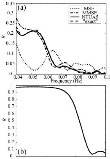
Figure 5: Reflection coefficient for the Scripps Canyon section as a function of frequency predicted by various models. (a) normal incidence $\theta_{i}=0^{\circ}$, (b) $\theta_{i}=45^{\circ}$. All models collapse on the same curve in (b).

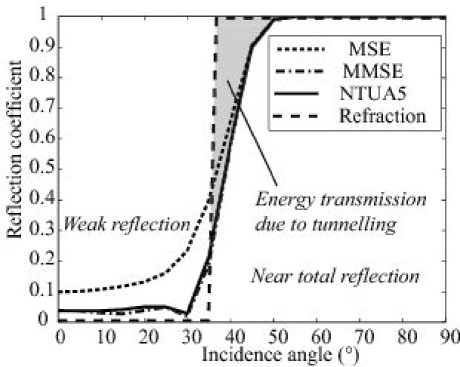
Figure 6: Reflection coefficient for waves of period $T=16$ s propagating over the Scripps Canyon section as a function of the wave incidence angle $\theta_{i}$ ($0$ corresponds to waves travelling perpendicular to the canyon axis).

Indeed, for a wave train propagating through a medium with phase speed gradient in one dimension only, geometrical optics predicts that beyond a threshold (Brewster) angle $\theta_{B}$, all the wave energy is trapped, and no energy goes through the canyon. This sharp transition does not depend on the magnitude of the gradient which may even be infinite. For a shelf depth $H_{1}$ and maximum canyon depth $H_{\mathrm{m}ax}$, this threshold angle is given by

$$\theta_{B}=\arcsin\left(\frac{C_{1}}{C_{\mathrm{max}}}\right)$$ (9)

where $C_{1}$ and $C_{\mathrm{max}}$ are the phase speeds for a given frequency corresponding to the depths $H_{1}$ and $H_{\mathrm{max}}$. Thus $\theta_{B}$ increases with increasing frequency as the phase speed difference diminishes at high frequencies. For Scripps Canyon, $H_{1}=24$ m, and $H_{\mathrm{max}}=145$ m. At $f=0.067$ Hz this gives $\theta_{B}=38^{\circ}$. As a result, for $\theta_{i}<\theta_{B}$, no reflection is predicted by refraction theory (dashed line), and all the wave energy is transmitted through the canyon. This threshold value separates distinct reflection and refraction (trapping) phenomena, respectively occurring for $\theta_{i}<\theta_{B}$ and $\theta_{i}>\theta_{B}$.

The elliptic models that account for diffraction predict a smoother transition. For $\theta_{i}<\theta_{B}$, weak reflection is predicted. For $\theta_{i}>\theta_{B}$, a fraction of the energy is still transmitted through the canyon. This transmission of wave energy across a deep region where $\sin\theta_{i}/C_{1}$ exceeds $1/C_{\mathrm{max}}$, violates the geometrical optics approximation. This transmission is similar to the tunnelling of quantum particles through a barrier of potential in the case where the barrier thickness is of the order of the wavelength or less [Thomson et al., 2005]. The wave field near the turning point of wave rays in the canyon decays exponentially in space on the scale of the wavelength [e.g. Chao and Pierson, 1972], and that decaying wave excites a propagating wave on the other side of the canyon. This coupling of both canyon sides generally decreases as the canyon width or the incidence angle increase [Kirby and Dalrymple, 1983; Thomson at al., 2005]. The significant differences between MSE and MMSE at small angles $\theta_{i}<\theta_{B}$ are less pronounced for $\theta_{i}>\theta_{B}$.

These two regimes are illustrated by the evolution of the wave potential amplitude over the Scripps canyon section. In figure 7, results of various elliptic models (MSE, MMSE and NTUA5) are compared with a parabolic approximation of the MSE (the REF/DIF1 model of Dalrymple and Kirby [1988]). It should be noted that the model grid orientation is chosen with the main axis along the incident wave propagation direction, in order to minimize large angle errors in the parabolic approximation. In that configuration, the parabolic approximation (REF/DIF1_a) does not predict any reflection, but gives an indication of the expected shoaling of the incident waves across the canyon. For $\theta_{i}=30^{\circ}<\theta_{B}$, weak reflection (about 10%) is predicted by the MMSE and NTUA5 (figure 7.a). MSE considerably overestimates the reflection, and thus underestimates the transmitted energy down-wave of the canyon section. A partial standing wave pattern is predicted up-wave of the canyon as a result of the interference of incident and reflected waves. The largest amplitudes, about $20\%$ larger than the incident wave amplitude, occur in the first antinode near the canyon wall.

For a larger wave incidence angle (e.g. 45${}^{\circ}>\theta_{B}$), an almost complete standing wave pattern is predicted by the elliptic models up-wave of the canyon, with an exponential tail that extends across the canyon to a weak transmitted component (see also Figure 5.b for the reflection coefficient pattern). Finally, transmission is extremely weak for $\theta_{i}=70^{\circ}$ (figure 7.c). A good estimate of the reflection coefficient can also be obtained with the parabolic model REF/DIF1_b by choosing the x-axis to be aligned with the canyon trench (figure 7b,c thick dashed lines).

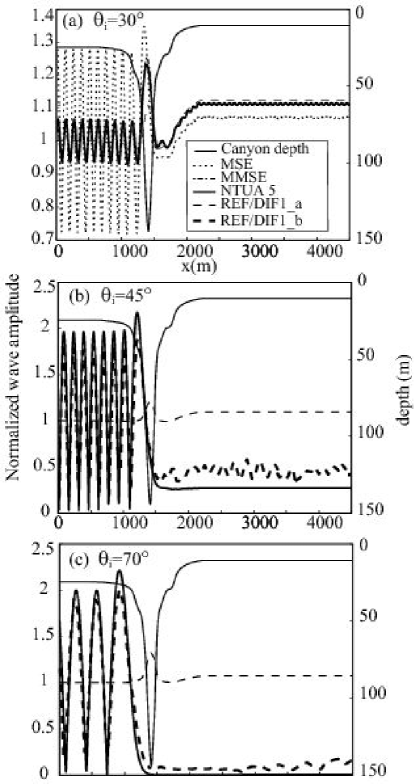
Figure 7: Wave amplitude over the Scripps Canyon section, for $T=16$ s and different incident angles (a) $\theta_{i}=30^{\circ}$, (b) $\theta_{i}=45^{\circ}$, and (c) $\theta_{i}=70^{\circ}$. The canyon depth profile is indicated with a thin dashed line. The MMSE result is in distinguishable from that of NTUA5 in all panels, and all models except for REF/DIF$1$ give the same results in (b) and (c).

4 West Swell Over Scripps Canyon

The models used in the previous section (MSE, MMSE, NTUA5, REF/DIF$1$, refraction) are now applied to the real $3$D bottom topography of the Scripps-La Jolla Canyon system, and compared with field data from directional wave buoys deployed around the rim and over Scripps Canyon during NCEX.

4.1 Models Set-up

The implementations of MSE, MMSE, NTUA5, and REF/DIF$1$ use two computational domains with grids of 275 by 275 points (Figure 8). The larger domain with a grid resolution of 21 m is used for wave periods longer than 15 s. The smaller domain, with a higher resolution of about 15 m, is used for 15 s and shorter waves. The $y$-axis of the grid is rotated 45^∘ relative to North to place the offshore boundary in the deepest region of the domain. Models were run for many sets of incident wave frequency and direction ($f$, $\theta$).

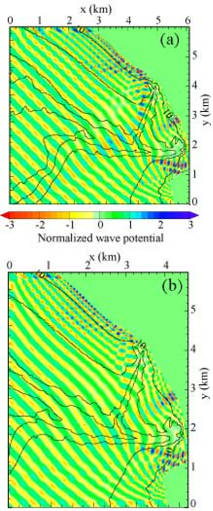
Figure 8: Computational domain for (a) $T>15$ s, and (b) $T\leq 15$ s. Also shown are the NTUA5 solutions for the real part of the wave potential amplitude for waves arriving from 270^∘ with periods (a) $T=16$ s, and (b) $T=15$ s, superimposed on the 10, 30, 100, 200, and 300 m depth contours.

The CPU time required for one ($f,\theta$) wave component calculation with the NTUA5 model (with $3$ evanescent modes) is about $120$ s on a Linux computer with $2$Gb of memory and a 3 GHz processor. The wave periods and offshore directions used in the computation range from $12$ to $22$ s and $255$ to $340$ degrees respectively, with $0.2$ s and $2^{\circ}$ increments. The minimum period $12$ s corresponds to the shortest waves that can be resolved with 7 points per wavelength in 10 m depth. Shorter waves are not considered here because they may be affected by local wind generation, not represented in the models used here, and are also generally less affected by the bottom topography.

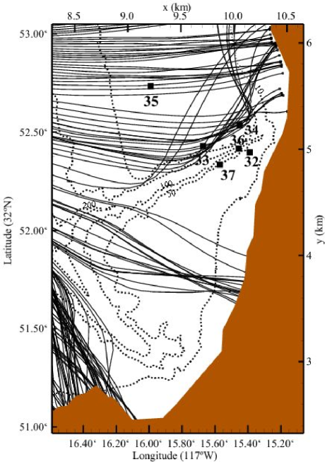
Figure 9: Location of directional wave buoys at the head of the Scripps canyon, and wave rays for an offshore direction of 272^∘ and a period of 15.4 s, corresponding to a frequency just below the peak of the observed swell on November 30. Contrary to the backward ray tracing model used for estimating the wave spectrum at nearshore sites, rays were integrated forward from parallel directions and equally spaced positions at 15 m intervals along the offshore boundary at $x=0$, 10 km to the West of the buoys, practically in deep water.

Transfer functions between the local and offshore wave amplitudes were evaluated at each of the buoy locations and used to transform the offshore spectrum. The backward ray-tracing refraction model directly evaluates energy spectral transfer functions between deep water, where the wave spectrum is assumed to be uniform, and each of the buoys located close to the canyon, based on the invariance of the wavenumber spectrum along a ray [Longuet-Higgins, 1957]. A minimum of $50$ rays was used for each frequency-direction bin (bandwidth 0.005 Hz by 5 degrees), computed over the finest available bathymetry grid, with 4 m resolution. The model is identical to the CREST model described by [Ardhuin et al.(2001)Ardhuin, Herbers, and O’Reilly], and validated by [Ardhuin et al.(2003)Ardhuin, Herbers, O’Reilly, and Jessen] on the U.S. East coast. The energy source term set to zero here. This propagation-only version of the model is also called CRESTp, and is similar to the model used by [O’Reilly and Guza(1993)] and [Peak(2004)]. It was further validated on the West coast of France [Ardhuin, 2006].

4.2 Model-Data Comparison

Long swell from the west was observed on $30$ November $2003$, in the absence of significant local winds. In the present analysis we use only data from Datawell Directional Waverider buoys. The Torrey Pines Outer Buoy is permanently deployed by the Coastal Data Information Program (CDIP), and located about $15$ km offshore of Scripps Canyon. That buoy provided the deep water observations necessary to drive the wave models. The directional distribution of energy for each frequency was estimated from buoy measurements of displacement cross-spectra using the Maximum Entropy Method [Lygre and Krogstad, 1986]. The NCEX observations were made at six sites around the head of Scripps Canyon (figure 9).

All spectra used in the comparison, including the offshore boundary condition, were averaged from 13:30 to 16:30 UTC, so that the almost continuous record yields about 100 degrees of freedom for each frequency band with a width of 0.005 Hz. On that day the wind speed close to the coast did not exceed 3 m s^-1, as measured by the CDIP Torrey Pines Glider port anemometer, and the National Data Buoy Center (NDBC) buoy 46086, located 70 km West of San Diego and representative of the entire modelled area.

The observed narrow offshore spectrum has a single peak with a period of $14.5$ s, and a mean direction of $272$ degrees, corresponding to an incidence angle $\theta_{i}$ (relative to the Scripps Canyon axis) of $65^{\circ}$ (Figure10).

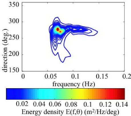
Figure 10: Directional wave spectrum at Torrey Pines Outer Buoy at 15:00 UTC on 30 November 2003.

The model hindcasts are compared with observations in Figure 11. While the local amplification of the wave height at the head of canyon varies with the incident wave direction, a dramatic reduction of the wave height downwave of the rim of this canyon is predicted for all directions. Thus the selected west swell case ($T_{p}=14.5s$, $\theta=272^{\circ}$) is representative of the general wave transformation in this area, for low frequency swells arriving a large range of directions. Significant wave heights $H_{s}$ were computed from the measured and predicted wave spectra at each instrument location, including only the commonly modelled frequency range ($f_{1}=0.05$ Hz, $f_{2}=0.08$ Hz). The predicted $H_{s}$ is given by

$$H_{s}=4\left(\int_{f_{1}}^{f_{2}}\int_{\theta_{1}}^{\theta_{2}}M(f,\theta)E(f,\theta)dfd\theta\right)^{1/2},$$ (10)

where $E(f,\theta)$ is the observed offshore frequency-directional spectrum and $M(f,\theta)$ is the model prediction of the ratio between the local and offshore wave energies for the frequency $f$ and offshore direction $\theta$, obtained by squaring the sea surface elevation transfer function.

Observations show a dramatic variation in wave height across the canyon (figure 11).

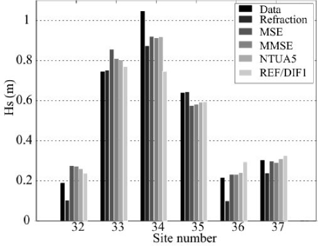
Figure 11: Comparison of predicted and observed significant wave height ($12s<T<22s$) for the 30 November 2003 swell event. Instrument locations are shown in figure 9.

The offshore wave height is slightly enhanced at sites 33 and 34, in water depths of 34 and 23 m respectively, along the north side of the canyon, and slightly reduced on the shelf north of the canyon at site 35, in 34 m depth. A dramatic reduction in wave heights is observed at sites 36, 37 and 32, over the Canyon and on the south side, where the water depths are 111, 49 and 24 m, respectively. Between buoys 34 and 36 the wave height drops by a factor 5 over a distance of only 150 m, that is less than the 216 m wavelength at the peak frequency (at the shallowest of the two sites). Such a pattern is generally consistent with refraction theory as illustrated by forward ray-tracing in figure 9. Whereas rays crossing the shelf north of the canyon show the expected gradual bending towards the shore, rays that reach the canyon northern wall are trapped on the shelf, and reach the shore in a focusing region north of the canyon (Black’s beach). From that offshore direction, and an offshore ray spacing of 15 m, no rays are predicted to cross the canyon, so that the south side of the canyon is effectively sheltered from 16 s Westerly swells, in agreement with the observed extremely low wave heights (figure 11, see also [Peak(2004)]). The amplitude transfer functions $(M(f,\theta)^{1/2}$) are not overly sensitive to the wave frequency and direction, as illustrated in figure 12.a-b with NTUA5 predictions at sites $34$ at the head of the canyon, and $37$ behind the canyon.

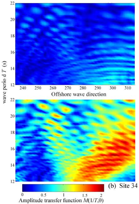
Figure 12: Amplitude transfer functions at site $34$ (a) and site $37$ (b), defined as the ratio of the local and offshore wave amplitude modulus and computed with NTUA $5$.

Up-wave of the canyon (instruments $33$, $34$, $35$), all models are found to be in fairly good agreement with the observations. However, REF/DIF$1$ underestimates the wave height at site $34$. At this site, wave energy is strongly focused by refraction, with rays turning by more that 90^∘ (figure 9). The parabolic approximation does not allow such a large variation in wave direction. Over and down-wave of the canyon (instruments $32$, $36$, $37$), the wave heights predicted by MSE, MMSE and NTUA5 agree reasonably well with the observations, whereas REF/DIF$1$ slightly overestimates the wave height. For $f<0.06$ Hz few rays cross the canyon and the energy predicted by the refraction model is extremely low, about $5$% of the offshore energy the total energy. This strong variation in wave energy across the canyon is reduced by diffraction, which is not taken into account in this refraction model, resulting in an under-prediction of the wave height at the sheltered sites $32$, $36$, and $37$.

The sea state at that time also include an important contribution from higher frequencies (figure 13). Significant wave heights computed over a wider frequency range ($0.05<f<0.2$Hz), by adding the refraction model results to the low-frequency results of other models, vary little between the models, now dominated by short wave energy.

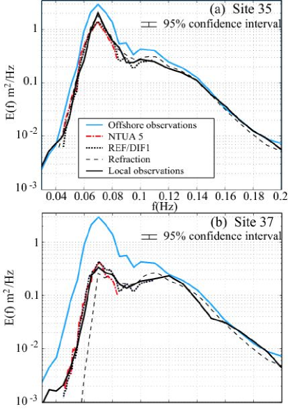
Figure 13: Comparison of predicted and observed frequency spectra at (a) site 35, and (b) site 37, for the 30 November 2003 swell event.

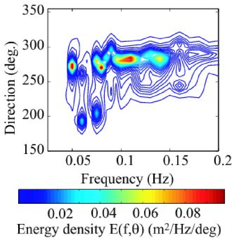
Figure 14: Directional wave spectrum at Torrey Pines Outer Buoy at 12:00 UTC on 12 December 2003.

However, wave heights are still markedly different between the buoys. It thus appears that refraction plays an important role for frequencies up to 0.14 Hz (see the difference in offshore and local spectra on figure 13), while diffraction effects are significant, in that area, only up to 0.07 Hz. Further confirmation of the trapping of low frequency waves is provided by another case observed on $12$ December $2003$ (Figure 14), which we analyze with the same method. The observed spectra are averaged from 12:00 UTC to 15:00 UTC.The observed spectrum has three peaks with a period of $20$, $12.5$ and $9$ s, a mean direction of $270$, $270$ and $285$ degrees respectively and a significant wave height of $1.9$m.

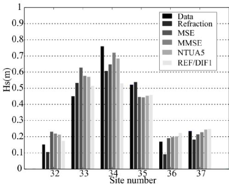
Figure 15: Comparison of predicted and observed significant wave height ($12s<T<22s$) for the 12 December 2003 swell event. Instrument locations are shown in figure 9.

The model hindcasts are compared with observations in Figure 15. Significant wave heights $H_{s}$ were computed from the measured and predicted wave spectra at each instrument location, including only the commonly modelled frequency range ($f_{1}=0.05$Hz, $f_{2}=0.08$Hz). On that day the wind speed did not exceed 7 m s^-1, as measured by the CDIP Torrey Pines Glider port anemometer, but reached 13.5 m, blowing from the North West, at NDBC buoy 46086. Such a wind is capable of generating a local wave field with frequencies down to 0.095 Hz for fully-developed wave conditions.

As in the previous case, a large variation in wave height was observed across the Canyon (Figure 15). Again, that variation remains limited to a factor 10 difference for any wave frequency (compare Figure 16a and b), whereas the geometrical optics approximation predicts much larger gradients. We note a general agreement of the predicted wave height by the models, with an underestimation of the refraction model for sites located down-wave of the Canyon. The predicted frequency spectra are represented on Figure 16a,b at sites $35$ and $37$. At site $35$, located up-wave of the Canyon wall, NTUA5 and REF/DIF1 models are in a good agreement with the measurement for the low frequency peak ($0.05$ Hz), but underestimate the $0.08$Hz peak. The refraction model overestimates the low frequency peak, but is in good agreement with the $0.08$Hz peak. At site $37$, located down-wave of the Canyon, NTUA5 and REF/DIF1 predict a strongly attenuated low frequency peak, as is observed, whereas the refraction model predicts no energy transmission across the canyon. Below a cut-off frequency of about $0.065$ Hz, the canyon acts as a complete barrier in the geometrical optics approximation. The energy in the second peak at $0.08$ Hz is only reduced by a factor 4 across the canyon, an effect well described by all models, and thus attributable to refraction. All models generally agree with the observations for $0.07<f<0.2$, within the spectrum measurement confidence interval, except for an overestimation of the refraction model for the high frequency peaks ($0.11$ and $0.14$ Hz) of the spectrum. However, due to the local wind sea generation between the offshore buoy and locations around the canyon, these propagation models are not reliable for $f>0.095$ Hz.

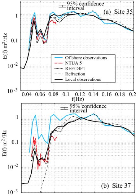
Figure 16: Comparison of predicted and observed frequency spectra at (a) site 35, and (b) site 37, 12 December 2003 swell event.

In the two events most of the wave evolution is accounted for by refraction. However, diffraction is included in the models based on the MSE and its extensions, and this effect allows for a tunnelling of wave energy across the canyon. In these models, wave heights across the canyon are thus larger, in better agreement with observed wave heights and wave spectra at the sheltered sites 32, 36 and 37 (figures 11, 13, 15).

The differences between NTUA5, MSE and MMSE model predictions are very small and thus only NTUA5 results are shown in figure 13. It may appear surprising that the wave height behind the canyon is still 20% of the offshore wave height whereas the 2D simulations with comparable incidence angles yield wave heights much less than 5%. However, the Scripps Canyon is neither infinitely long nor uniform along its axis. The three-dimensional topography apparently reduces the blocking effect of long period swells that was found over two-dimensional canyons.

5 Summary

Observations of the evolution of swell across a submarine canyon obtained in the nearshore canyon experiment (NCEX), were compared with predictions of refraction and combined refraction-diffraction models including the coupled-mode model NTUA5 valid for arbitrary bottom slope [Athanassoulis and Belibassakis, 1999; Belibassakis et al., 2001]. Predictions of a spectral refraction model are in good agreement with observations [see also Peak, 2004 for the entire experiment], demonstrating that refraction is the dominant process in swell transformation across Scripps Canyon. The geometrical optics approximation, on which the refraction model is based, turned out to be very robust. Accurate spectral predictions were obtained with taht model even in cases where the wave energy changes by a factor of 10 over three quarters of a wavelength.

For waves longer than 12 s, even larger gradients are predicted by the refraction model, but these gradients are not observed. At those frequencies, accurate results were obtained with the NTUA5 model and elliptic mild slope equation models that include diffraction, which acts as a limiter on the wave energy gradients. Differences between the models were clarified with 2D simulations using representative transverse profiles of La Jolla and Scripps Canyons, showing the behavior of the far wave field as a function of the incidence angle. The underestimation by the refraction model may be interpreted as the result of wave tunnelling, i.e. a transmission of waves to water depths greater than allowed by Snel’s law, for obliquely incident waves [see also, Thomson et al., 2005]. This tunnelling effect cannot be represented in the geometrical optics approximation, and thus the refraction model predicts that all wave energy is trapped for large incidence angles relative to the depth contours, while a small fraction of the wave energy is in fact transmitted across the canyon. Although different from the classical diffraction effect behind a breakwater [e.g. Mei 1989], this tunnelling is a form of diffraction in the sense that it prevents a sharp spatial variation of wave amplitude, and induces a leakage of wave energy in areas forbidden by geometrical optics.

Observations were also compared with a parabolic refraction-diffraction model that is known to be inaccurate for large oblique wave directions relative to the numerical grid, and is shown here to overestimate the amplitude of waves transmitted across the canyon and underestimate the amplitude of waves focused at the head of the canyon. Finally, depending on the bottom profile and incidence angle, higher order bottom slope and curvature terms (incorporated in modified mild slope equations and NTUA5), as well as evanescent and sloping-bottom modes (included in NTUA5) can be important for an accurate representation of wave propagation over a canyon at small incidence angles. For large incidence angles, that are more common for natural canyons across the shelf break, the standard mild slope equation (MSE) gives an accurate representation of the variations in surface elevation spectra that is similar to that of the full NTUA$5$ model. Yet, further analysis of NCEX bottom velocity and pressure measurements may show that the MSE or other mild slope models may not accurately represent near bottom wave properties, as also discussed by [Athanassoulis et al.(2003)Athanassoulis, Belibassakis, and Georgiou].