Internet data packet transport: from global topology to local queueing dynamics

Abstract

We study structural feature and evolution of the Internet at the autonomous systems level. Extracting relevant parameters for the growth dynamics of the Internet topology, we construct a toy model for the Internet evolution, which includes the ingredients of multiplicative stochastic evolution of nodes and edges and adaptive rewiring of edges. The model reproduces successfully structural features of the Internet at a fundamental level. We also introduce a quantity called the load as the capacity of node needed for handling the communication traffic and study its time-dependent behavior at the hubs across years. The load at hub increases with network size $N$ as $\sim N^{1.8}$. Finally, we study data packet traffic in the microscopic scale. The average delay time of data packets in a queueing system is calculated, in particular, when the number of arrival channels is scale-free. We show that when the number of arriving data packets follows a power law distribution, $\sim n^{-\lambda}$, the queue length distribution decays as $n^{1-\lambda}$ and the average delay time at the hub diverges as $\sim N^{(3-\lambda)/(\gamma-1)}$ in the $N\to\infty$ limit when $2<\lambda<3$, $\gamma$ being the network degree exponent.

In recent years, the Internet has become one of the most influential media in our daily life, going beyond in its role as the basic infrastructure in this technological world. Explosive growth in the number of users and hence the amount of traffic poses a number of problems which are not only important in practice for, e.g., maintaining it free from any undesired congestion and malfunctioning, but also of theoretical interests as an interdisciplinary topic internetbook . Such interests, also stimulated by other disciplines like biology, sociology, and statistical physics, have blossomed into a broader framework of network science rmp ; portobook ; siam ; report . In this Letter, we first review briefly previous studies of Internet topology and the data packet transport on global scale, and next study the delivery process in queueing system of each node embedded in the Internet.

The Internet is a primary example of complex networks. It consists of a large number of very heterogeneous units interconnected with various connection bandwidths, however, it is neither regular nor completely random. In their landmark paper, Faloutsos et al. fal3 showed that the Internet at the autonomous systems (ASes) level is a scale-free (SF) network physica , meaning that degree $k$, the number of connections a node has, follows a power-law distribution,

$$P_{d}(k)\sim k^{-\gamma}.$$ (1)

The degree exponent $\gamma$ is subsequently measured and confirmed in a number of studies to be $\gamma\approx 2.1(1)$. The power-law degree distribution implies the presence of a few nodes having a large number of connections, called hubs, while most other nodes have a few number of connections.

It is known that the degrees of the two nodes located at each end of a link are correlated each other. As the first step, the degree-degree correlation can be quantified in terms of the mean degree of the neighbors of a given node with degree $k$ as a function of $k$, denoted by $\langle k_{\rm nn}\rangle(k)$ vespig , which behaves in another power law as

$$\langle k_{\rm nn}\rangle(k)\sim k^{-\nu}.$$ (2)

For the Internet, it decays with $\nu\approx 0.5$ measured from the real-world Internet data routeviews ; nlanr .

The Internet has modules within it. Such modular structures arise due to regional control systems, and often form in a hierarchical way maslov_PRL . Recently, it was argued that such modular and hierarchical structures can be described in terms of the clustering coefficient. Let $C_{i}$ be the local clustering coefficient of a node $i$, defined as $C_{i}=2e_{i}/k_{i}(k_{i}-1)$, where $e_{i}$ is the number of links present among the neighbors of node $i$, out of its maximum possible number $k_{i}(k_{i}-1)/2$. The clustering coefficient of a network, $C$, is the average of $C_{i}$ over all nodes. $C(k)$ means the clustering function of a node with degree $k$, i.e., $C_{i}$ averaged over nodes with degree $k$. When a network is modular and hierarchical, the clustering function follows a power law, $C(k)\sim k^{-\beta}$ for large $k$, and $C$ is independent of system size $N$ Ravasz02 ; Ravasz03 . For the Internet, it was measured that the clustering coefficient is $C_{\rm AS}\approx 0.25$ and the exponent $\beta\approx 0.75$ vpsv .

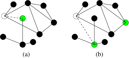
Figure 1: Shown is the adaptive rewiring rule. A node (white) detaches one of its links from a node (green or gray) in (a), and attaches it to one of the nodes (green or gray) with degree 3, larger than 2 of the detached node, in (b).

There are many known models to mimic the Internet topology. Here we introduce our stochastic model evolving through the following four rules. This model is based on the model proposed by Huberman and Adamic ha , which is a generic model to reproduce a uncorrelated SF network and we modify it by adding the adaptation rule fluc , which results in generating the degree-degree correlations. The rules are as follows: (i) Geometrical growth: At time step $t$, geometrically increased number of new nodes, $\alpha N(t-1)$, are introduced in the system with the empirical value of $\alpha=0.029$. Then following the empirical fact $\langle k_{\rm new}\rangle_{t}\approx 1.34$, each of newly added nodes connects to one or two existing nodes according to the preferential attachment (PA) rule ba . (ii) Accelerated growth: Each existing node increases its degree by the factor empirical value of $\approx 0.035$. These new internal links are also connected following the PA rule. (iii) Fluctuations: Each node disconnects existing links randomly or connects new links following the PA rule with equal probability. The variance of this noise is given as $\sigma^{2}\approx(0.14)^{2}$ measured from empirical data. (iv) Adaptation: When connecting in step (iii), the PA rule is applied only within the subset of the existing nodes consisting of those having larger degree than the one previously disconnected. This last constraint accounts for the adaptation process. The adaptive rewiring rule is depicted in Fig. 1.

Through this adaptation model, we can reproduce generic features of the Internet topologies successfully which are as follows: First, the degree exponent is measured to be $\gamma_{\rm model}\approx 2.2$, close to the empirical result $\gamma_{\rm AS}\approx 2.1(1)$. Second, the clustering coefficient is measured to be $C_{\rm model}\approx 0.15(7)$, comparable to the empirical value $C_{\rm AS}\approx 0.25$. Note that without the adaptation rule, we only get $C\approx 0.01(1)$. The clustering function $C(k)$ also behaves similarly to that of the real-world Internet, specifically, decaying in a power law with $\beta\approx 1.1(3)$ roughly for large $k$ book1 , but the overall curve shifts upward and the constant behavior for small $k$ appears. Third, the mean degree function $\langle k_{\rm nn}\rangle(k)$ also behaves similarly to that of the real-world Internet network, but it also shifts upward overall. In short, the behaviors of $C(k)$ and $\langle k_{\rm nn}\rangle(k)$ of the adaptation model are close to those of the real Internet AS map, but with some discrepancies described above. On the other hand, recently another toy model serrano05 has been introduced to represent the evolution of the Internet topology. The model is similar to our model in the perspective of including the multiplicative stochastic evolution of nodes and edges as well as adaptive rewiring of edges. However, the rewiring dynamics is carried out with the incorporation of user population instead of degree of node we used here.

Figure 2: The load at each node due to a unit packet transfer from the node $s$ to the node $t$, $\ell_{i}^{s\rightarrow t}$. In this diagram, only the nodes along the shortest paths between $(s,t)$ are shown. The quantity in parentheses is the corresponding value of the load due to the packet from $t$ to $s$, $\ell_{i}^{t\rightarrow s}$.

Next, we study the transport of data packet on the Internet. Data packets are sent and received over it constantly, causing momentary local congestion from time to time. To avoid such undesired congestion, the capacity, or the bandwidth, of the routers should be as large as it can handle the traffic. First we introduce a rough measure of such capacity, called the load and denoted as $\ell$ load . One assumes that every node sends a unit packet to everyone else in unit time and the packets are transferred from the source to the target only along the shortest paths between them, and divided evenly upon encountering any branching point. To be precise, let $\ell_{i}^{s\rightarrow t}$ be the amount of packet sent from $s$ (source) to $t$ (target) that passes through the node $i$ (see Fig. 2). Then the load of a node $i$, $\ell_{i}$, is the accumulated sum of $\ell_{i}^{s\rightarrow t}$ for all $s$ and $t$, $\ell_{i}=\sum_{s\neq t}\ell_{i}^{s\rightarrow t}$. In other words, the load of a node $i$ gives us the information how much the capacity of the node should be in order to maintain the whole network in a free-flow state. However, due to local fluctuation effect of the concentration of data packets, the traffic could be congested even for the capacity of each node being taken as its load. The distribution of the load reflects the high level of heterogeneity of the Internet: It also follows a power law,

$$P_{l}(\ell)\sim\ell^{-\delta},$$ (3)

with the load exponent $\delta\approx 2.0$ for the Internet. For comparison, the quantity “load” is different from the “betweenness centrality” freeman in its definition. In load, when a unit packet encounters a branching point along the shortest pathways, it is divided evenly with the local information of branching number, while in betweenness centrality, it can be divided unevenly with the global information of the total number of shortest pathways between a given source and target book2 . Despite such a difference, we find no appreciable difference in practice for the numerical values of the load and the betweenness centrality for a given network.

The load of a node is highly correlated with its degree. This suggests a scaling relation between the load and the degree of a node as $\ell\sim k^{\eta}$ and the scaling exponent $\eta$ is estimated as $\eta=1.06\pm 0.03$ for January 2000 AS map vpsv ; book1 . In fact, if one assumes that the ranks of each node for the degree and the load are the same, then one can show that the exponent $\eta$ depends on $\gamma$ and $\delta$ as $\eta=(\gamma-1)/(\delta-1)$ with $\gamma\approx 2.1$ and $\delta\approx 2.0$, and we have $\eta\approx 1.1$, which is consistent with the direct measurement.

Figure 3: Time evolution of the load versus $N(t)$ at the ASes of degree-rank 1($\circ$), 2 ($\Box$), 3 ($\Diamond$), 4 ($\triangle$), and 5 ($\times$). The dashed line for larger $N$ has slope 1.8, drawn for the eye.

The time evolution of the load at each AS is also of interest. Practically, how the load scales with the total number of ASes (the size of the AS map) is an important information for the network management. In Fig. 3, we show $\ell_{i}(t)$ versus $N(t)$ for 5 ASes with the highest rank in degree, i.e., 5 ASes that have largest degrees at $t=0$. The data of $\{\ell_{i}(t)\}$ shows large fluctuations in time. Interestingly, the fluctuation is moderate for the hub, implying that the connections of the hub is rather stable. The load at the hub is found to scale with $N(t)$ as $\ell_{h}(t)\sim N(t)^{\mu}$, but the scaling shows a crossover from $\mu\approx 2.4$ to $\mu\approx 1.8$ around $t\approx 14$.

Internet traffic along the shortest pathways yields inconvenient queue congestions at hubs in SF networks. Many alternative routing strategies have been introduced to reduce the load at hub and improve the critical density of the number of packets displaying the transition from free-flow to congested state tadic04 ; rodgers ; arenas ; holme ; echenique ; greiner ; duch ; zoltan .

Transport of data packets also relies on queueing process of an individual AS. Here we extend existing queueing theory qt to the case where arrival channels are multiple, in particular, when their number distribution follows a power law, aiming at understanding the transport in SF networks. For simplicity, we assume that the arrival and processing rates of an individual channel are the same, and they are independent of degree of a given AS. Time is discretized and unit time is given as the inverse of the rate.

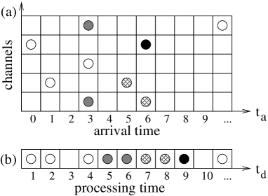
Figure 4: (a) Snapshot inside buffer with arriving packets. Each row represents a communication channel, and circles therein are the sequence of incoming packets. The integers on the horizontal axis indicate arriving time-steps of each packet. Open circles stand for packets not delayed. Packets delayed are represented by three kinds of filled circles according to their own delaying mechanism. See text for details. The consequent delivery sequence is shown in (b) with processing time-step.

Delay of packet delivery in our queueing process originates from two sources. For the one, owing to multiple arriving channels, multiple packets can arrive at a given queueing system in a unit time interval, and are accumulated in the buffer. For example, grey circles in Fig. 4 represent such a case. This type of delay is referred to as the delay type 1 (DT1) below. For the other, the delay is caused by preceding packets in the buffer, which can happen under the first-in-first-out rule. The hatched circles in Fig. 4 demonstrate this case. This case is referred to as the delay type 2 (DT2). Then any delay can be decomposed into the two types. The black circle in Fig.4 is such a packet, delayed by both DT1 and DT2. We calculate the average delay time for each type, separately, and combine them next.

To proceed, we first define $p_{n}$ as the probability that $n$ packets arrive at a given queueing system at the same time. For the DT1 case, if $q_{m}$ denotes the probability that a packet is delayed $m$ time steps, we find

$$q_{m}=p_{0}\delta_{0,m}+\sum_{n=m+1}^{\infty}{p_{n}\over n},$$ (4)

where $\delta_{i,j}$ is the Kronecker delta function. Then, the average of delay time steps through the DT1 process is obtained as

$$\langle m\rangle_{q}=\sum_{n=2}^{\infty}{p_{n}\over n}\sum_{m=1}^{n-1}m={{\langle n\rangle_{p}-1+p_{0}}\over 2},$$ (5)

where $\langle\cdots\rangle_{q}$ ($\langle\cdots\rangle_{p}$) is the average with respect to the probability $q_{m}$ ($p_{n}$).

For the DT2 case, we introduce $r_{b}(t)$ as the probability that a packet arrived at time $t$ is delayed $b$ time steps by preceding delayed packets. In the steady state, we obtain that

$$r_{b^{\prime}}=\sum_{b=0}^{{b^{\prime}}+1}p_{{b^{\prime}}-b+1}r_{b}+p_{0}r_{0}\delta_{0,{b^{\prime}}}.$$ (6)

By using the generating functions ${\cal{R}}(z)\equiv\sum_{b=0}^{\infty}r_{b}z^{b}$ and ${\cal{P}}(z)\equiv\sum_{n=0}^{\infty}p_{n}z^{n}$, we obtain that

$${\cal{R}}(z)\left[z-{\cal{P}}(z)\right]=p_{0}r_{0}(z-1)\ ,$$ (7)

with $p_{0}r_{0}=1-\langle n\rangle_{p}$.

The next step is to combine the two types of delays. To this end, we define $w_{\tau}$ as the probability that a unit packet is delayed by $\tau$. Then $w_{\tau}=\sum_{m=0}^{\tau}q_{m}r_{\tau-m}$ since DT1 and DT2 are statistically independent. From this, the average delay time is obtained as

$$\langle\tau\rangle_{w}\equiv\sum_{\tau=0}^{\infty}\tau w_{\tau}={{\langle n\rangle_{p}-1+p_{0}}\over 2}+{{\langle n^{2}\rangle_{p}-\langle n\rangle}_{p}\over{2\left(1-\langle n\rangle_{p}\right)}}\ .$$ (8)

Thus, a critical congestion occurs when $\langle n\rangle_{p}=1$, at which the delay time diverges. The singular behavior in the form of $(1-\langle n\rangle_{p})^{-1}$ was observed numerically in the study of directed traffic flow in Euclidean space manna .

We now consider the case where the number of arriving data packets follows a power law, $p_{n}\sim n^{-\lambda}$. In fact, non-uniformity of the number of data packets arriving at a given node gives rise to self-similar patterns as is well known in computer science walter . Precise value of the exponent $\lambda$ has not been reported yet. Moreover, it is not known if the exponent is universal, independent of bandwidths or degrees in the SF network. The relation of $\lambda$ to the load exponent $\delta$, if there is any, is not known either.

If $\lambda<3$, $\langle n^{2}\rangle_{p}$ diverges. For such a power-law distribution, its generating function ${\cal P}(z)$ develops a singular part and takes the form, when $2<\lambda<3$,

$${\cal{P}}(z)=1-\langle n\rangle_{p}(1-z)+a(1-z)^{\lambda-1}+\mathcal{O}\left((1-z)^{2}\right),$$ (9)

where $a$ is a constant. By using the relation between ${\cal{P}}(z)$ and ${\cal{R}}(z)$ from Eq. (7), we obtain that

$${\cal{R}}(z)=1-{a\over{1-\langle n\rangle}_{p}}(1-z)^{\lambda-2}+\mathcal{O}\left(1-z\right).$$ (10)

Therefore, the probability $r_{b}$ in the delay of the DT2 behaves as $r_{b}\sim b^{1-\lambda}$ for large $b$. In other words, the DT2 delay distribution decays slower than that of incoming packets, $p_{n}$, and $\langle\tau\rangle_{w}\sim\langle b\rangle_{r}$ becomes infinite even when $\langle n\rangle_{p}<1$.

On the other hand, in real finite scale-free networks such as the Internet with the degree exponent $\gamma$, $p_{n}$ at the hub has a natural cut-off at $n\sim k_{\rm max}\sim N^{1/(\gamma-1)}$, in which case we have $\langle n^{2}\rangle_{p}\sim k_{\rm max}^{3-\lambda}$. Thus from Eq. (8) the average delay time at the hub scales as

$$\langle\tau\rangle_{w}\sim k_{\rm max}^{3-\lambda}\sim N^{(3-\lambda)/(\gamma-1)}$$ (11)

for $2<\lambda<3$.

In the real-world Internet, the bandwidth of each AS is not uniform. Nodes with high bandwidth locate at the core of the network, forming a rich club richclub1 ; richclub2 , however, their degrees are small. Whereas, nodes with large degree locate at the periphery of the network with low bandwidth hot . Therefore, our analysis of the average delay time has to be generalized incorporating the inhomogeneous bandwidths and arrival rates outlook .

In summary, in the first part of this Letter, we have reviewed the previous studies of topological properties of the Internet and introduced a minimal model, the adaptation model to reproduce the topological properties. Next we studied transport phenomena of data packets travelling along the shortest pathways from source to destination nodes in terms of the load. In the second part, we studied the delivery process of data packets in the queueing system, in particular, when arrival channels are diverse following the scale-freeness in the degree distribution.

This work is supported by the KOSEF grants No. R14-2002-059-01000-0 in the ABRL program.

References

- (1) R. Pastor-Satorras and A. Vespignani, Evolution and Structure of the Internet (Cambridge University Press, Cambridge, 2004).
- (2) R. Albert and A.-L. Barabási, Rev. Mod. Phys. 74, 47 (2002).
- (3) S. N. Dorogovtsev and J. F. F. Mendes, Evolution of Networks (Oxford University Press, Oxford, 2003).
- (4) M. E. J. Newman, SIAM Rev. 45, 167 (2003).
- (5) S. Boccaletti, V. Latora, Y. Moreno, M. Chavez, and D.-U. Hwang, Physics Reports 424, 175 (2006).
- (6) M. Faloutsos, P. Faloutsos, and C. Faloutsos, Comput. Commun. Rev. 29, 251 (1999).
- (7) A.-L. Barabási, R. Albert, and H. Jeong, Physica A 272, 173 (1999).
- (8) R. Pastor-Satorras, A. Vázquez, and A. Vespignani, Phys. Rev. Lett. 87, 258701 (2001).
- (9) D. Meyer, University of Oregon Route Views Archive Project (http://archive.routeviews.org).
- (10) The NLANR project sponsored by the National Science Foundation (http://moat.nlanr.net).
- (11) K. A. Eriksen, I. Simonsen, S. Maslov, and K. Sneppen, Phys. Rev. Lett. 90, 148701 (2003).
- (12) E. Ravasz, A. L. Somera, D. A. Mongru, Z. N. Oltvai, and A.-L. Barabási, Science 297, 1551 (2002).
- (13) E. Ravasz and A.-L. Barabási, Phys. Rev. E 67, 026112 (2003).
- (14) A. Vázquez, R. Pastor-Satorras, and A. Vespignani, Phys. Rev. E 65, 066130 (2002).
- (15) B. A. Huberman and L. A. Adamic, e-print (http://arxiv.org/abs/cond-mat/9901071) (1999).
- (16) K.-I. Goh, B. Kahng, and D. Kim, Phys. Rev. Lett. 88, 108701 (2002).
- (17) A.-L. Barabási and R. Albert, Science 286, 509 (1999).
- (18) K.-I. Goh, E.S. Oh, C.M. Ghim, B. Kahng and D. Kim, in Lecture Notes in Physics: Proceedings of the 23rd CNLS Conference, “Complex Networks,” Santa Fe 2003, edited by E. Ben-Naim, H. Frauenfelder, and Z. Toroczkai (Springer, Berlin, 2004).
- (19) M. A. Serrano, M. Boguñá and A. Díaz-Guilera, Phys. Rev. Lett. 94, 038701 (2005).
- (20) K.-I. Goh, B. Kahng, and D. Kim, Phys. Rev. Lett. 87, 278701 (2001).
- (21) L.C. Freeman, Sociometry 40, 35 (1977).
- (22) K.-I. Goh, B. Kahng and D. Kim, in Complex Dynamics in Communication Networks, edited by L. Kocarev and G. Vattay (Springer, Berlin, 2005).
- (23) B. Tadić and S. Thurner, Physica A 332, 566 (2004).
- (24) B. Tadić and G.J. Rodgers, Adv. Complex Syst. 5, 445 (2002).
- (25) P. Holme, Adv. Complex Syst. 6, 163 (2003).
- (26) A. Arenas, A. Díaz-Guilera and R. Guimera, Phys. Rev. Lett. 86, 3196 (2001).
- (27) P. Echenique, J. Gómez-Gardeñes, and Y. Moreno, Phys. Rev. E 70, 056105 (2004).
- (28) M. Schäfer, J. Scholz, and M. Greiner, Phys. Rev. Lett. 96, 108701 (2006).
- (29) J. Duch and A. Arenas, arXiv:physics/0602077.
- (30) S. Sreenivasan, R. Cohen, E. López, Z. Toroczkai, and H. E. Stanley, arXiv:cs.NI/0604023.
- (31) D. Gross and C. M. Harris, Fundamentals of Queueing Theory, 3rd ed. (Wiley, New York, 1998).
- (32) G. Mukherjee and S. S. Manna, Phys. Rev. E 71, 066108 (2005).
- (33) W. E. Leland, M.S. Taqqu, W. Willinger, and D. V. Wilson, IEEE/ACM Transactions on networking 2, 1 (1994).
- (34) S. Zhou and R. J. Mondragon, IEEE Commum. Lett. 8, 180 (2004).
- (35) V. Colizza, A. Flammini, M. A. Serrano and A. Vespignani, Nat. Phys. 2, 112 (2006).
- (36) L. Li, D. Alderson, R. Tanaka, J. C. Doyle, W. Willinger, arXiv:cond-mat/0501169.
- (37) H. K. Lee, B. Kahng and D. Kim (unpublished).