Comparison of Two Scale-Dependent Dynamic Subgrid-Scale Models for Simulations of Neutrally Buoyant Shear-Driven Atmospheric Boundary Layer Flows

Abstract

A new scale-dependent dynamic subgrid-scale (SGS) model based on Kolmogorov’s scaling hypothesis is presented. This SGS model is utilized in large-eddy simulation of a well-known case study on shear-driven neutral atmospheric boundary layer flows. The results are compared comprehensively with an alternate scale-dependent dynamic SGS model based on the popular Smagorinsky closure. Our results show that, in the context of this particular problem, the scale-dependent dynamic modeling approach is extremely useful, and reproduces several establised results (e.g., the surface layer similarity theory) with fidelity. Results from both the SGS base models are generally in close agreement, although we find a consistent superiority of the Smagorinsky-based SGS model for predicting the inertial range scaling of spectra.

Abbreviations ABL - Atmospheric boundary layer; LES - Large-eddy simulation; SGS - Subgrid scale; NBL - Neutral boundary layer; TKE - Turbulence kinetic energy.

1 Introduction

The dynamic subgrid-scale (SGS) modeling approach of Germano et al. germ91 has been quite successful in large-eddy simulations (LESs) of various engineering flows pope04 . In this approach, one dynamically computes the values of the unknown SGS coefficients at every time and position in the flow. By looking at the dynamics of the flow at two different resolved scales, and assuming scale similarity as well as scale invariance of the SGS coefficients, one can optimize their values. Thus, the dynamic modeling approach avoids the need for a priori specification and tuning of the SGS coefficients. A recent study meye05 based on extensive database analysis further suggests that the dynamic modeling approach closely reproduces the minimal simulation error strategy (termed as optimal refinement strategy), which is highly desirable in turbulence modeling.

In atmospheric boundary layer (ABL) turbulence, where shear and stratification and associated flow anisotropies are (almost) ubiquitous, the inherent scale-invariance assumption of the original dynamic modeling approach breaks down. Porté-Agel et al. port00 relaxed this assumption and introduced a scale-dependent dynamic modeling approach in which the SGS coefficients are assumed to vary as powers of the LES filter width ($\Delta_{f}$). The unknown power-law exponents, and subsequently the SGS coefficients, can be determined in a self-consistent manner by filtering at three levels port00 ; port04 . In the simulations of neutral boundary layers (NBLs), the scale-dependent dynamic SGS model was found to exhibit appropriate dissipation behavior and more accurate spectra in comparison to the original (scale-invariant) dynamic model port00 ; port04 . Recently the scale-dependent dynamic modeling approach was modified and extended by incorporating a localized averaging technique in order to simulate intermittent, patchy turbulence in the stably stratified flows basu06a ; basu06b . In parallel, scale-dependent dynamic SGS models based on Lagrangian averaging over fluid flow path lines were developed by Bou-zeid et al. bouz05 and Stoll and Porté-Agel stol06 to simulate neutrally stratified flows over heterogeneous surfaces.

The scale-dependent dynamic modeling approach and its variants so far always used the popular eddy-viscosity formulation of Smagorinsky smag63 as the SGS base model. However, this SGS model assumes that the energy dissipation rate equals the SGS energy production rate. In order to avoid this strong assumption, Wong and Lilly wong94 proposed a new SGS model based on Kolmogorov’s scaling hypothesis. A dynamic version of the Wong-Lilly SGS model to some extent outperformed the dynamic Smagorinsky model in simulations of the buoyancy-driven Rayleigh-Bénard convection wong94 . Furthermore, the dynamic Wong-Lilly SGS model is computationally inexpensive in comparison to the dynamic Smagorinsky SGS model. The combination of lesser assumptions and cheaper computational cost certainly make the Wong-Lilly model an attractive SGS base model for LES. Therefore it is of interest to explore if the Wong-Lilly SGS model or its variants are capable of simulating different flow regimes of the ABL. It is generally agreed upon that in comparison to buoyancy-driven flows, large-eddy simulations of shear-driven boundary layer flows are far more challenging. Thus, in the present study, we focus on neutrally buoyant shear-driven ABL flow. In order to realistically account for the near-wall shear effects, we first formulate a locally averaged scale-dependent dynamic version of the Wong-Lilly SGS model (henceforth LASDD-WL, see Appendix for details). Then, we comprehensively compare its performance with the locally averaged scale-dependent dynamic Smagorinsky (hereafter LASDD-SM) SGS model earlier developed by Basu and Porté-Agel basu06a .

The structure of this paper is as follows. In Section 2, we briefly provide the technical details of a case study. Extensive comparisons (in terms of the similarity theory, spectra, and flow visualizations) between the LASDD-WL and LASDD-SM SGS models are performed in Section 3. Finally, concluding remarks are made in Section 4.

2 Description of Simulations

In this work, we perform large-eddy simulations of a turbulent Ekman layer (i.e., pure shear flow with a neutrally stratified environment in a rotating system) utilizing the LASDD-SM basu06a ; basu06b and LASDD-WL (see Appendix) SGS models. Both these simulations are identical in terms of initial conditions, forcings, and numerical specifications (e.g., time integration, grid spacing). Technical details of our LES code and the LASDD-SM SGS modeling approach have been described in detail in basu06a and will not be repeated here for brevity.

The selected case study is similar to that of the LES intercomparison study by Andrén et al. andr94 . The simulated boundary layer is driven by an imposed geostrophic wind of $\left(U_{g},V_{g}\right)=\left(10,0\right)$ ms^-1. The Coriolis parameter is equal to $f_{c}=10^{-4}$ s^-1, corresponding to latitude $45^{\circ}$ N. The computational domain size is: $L_{x}=L_{y}=4000$ m and $L_{z}=1500$ m. This domain is divided into $N_{x}\times N_{y}\times N_{z}=40\times 40\times 40$ nodes (i.e., $\Delta_{x}=\Delta_{y}=100$ m, and $\Delta_{z}=38.5$ m). The motivation behind the selection of this coarse grid-resolution is two-fold. Primarily it allows us to perform a direct comparison with the results from andr94 , which used almost the same grid-resolutions. More importantly, coarse grid-resolution enables us to identify the strengths and/or weaknesses of different SGS models, as well as, to underscore their impacts on large-eddy simulations. The simulations are run for a period of $10\times f_{c}^{-1}$ (i.e., 100,000 s), with time steps of 2 s. The last $3\times f_{c}^{-1}$ interval is used to compute statistics. A passive scalar is introduced in the flows by imposing a constant flux ($\overline{wc}_{0}$) of $10^{-3}$ kg m^-2 s^-1 at the surface. The lower boundary condition is based on the Monin-Obukhov similarity theory with a surface roughness length of $z_{\circ}=0.1$ m.

3 Results and Discussions

In this section, we report the results of the LASDD-SM and LASDD-WL SGS models-based simulations and compare them with results from the intercomparison study andr94 , wherever possible. This particular case (without the inclusion of passive scalars) was also simulated by Kosović koso97 using a nonlinear SGS model, and recently by Chow et al. chow05 , who utilized a sophisticated hybrid SGS model. Our simulations show that both the LASDD SGS models perform very well, and the results are comparable to the past studies.

Temporal evolution of the surface friction velocity ($u_{*}$) is very similar in both the simulations (not shown). The average value of $u_{*}$ during the last $3\times f_{c}^{-1}$ interval is approximately 0.44 ms^-1 in the case of the LASDD-SM model. The LASDD-WL model produces a marginally higher value (0.454 ms^-1). The corresponding values found in andr94 are: 0.425 ms^-1 (Moeng), 0.448 ms^-1 (Mason - backscatter), 0.402 ms^-1 (Mason - non-backscatter), 0.402 ms^-1 (Nieuwstadt), and 0.425 ms^-1 (Schumann).

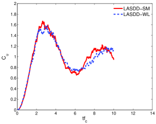
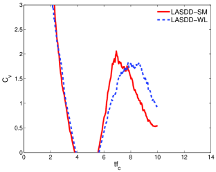
Figure 1: Temporal evolution of the nonstationarity parameters $C_{u}$ (left) and $C_{v}$ (right).

In Figure 1, we present the nonstationary parameters $C_{u}$ and $C_{v}$ (see andr94 for definitions). Under steady state conditions, these parameters should approach unity. Although none of the past andr94 ; chow05 and present simulations are quite close to steady state conditions, they are more or less in phase with each other. All these simulations clearly portray the inertial oscillation of period $2\pi/f_{c}$, as anticipated.

Accurately simulating the non-dimensional velocity gradient $(\phi_{M})$, and the scalar gradient $(\phi_{C})$ in the neutrally stratified surface layer has proven to be a very challenging task for many atmospheric LES models. It is well known that the traditional Smagorinsky model is over-dissipative in the near-surface region and gives rise to excessive mean gradients in velocity and scalar fields (cf. andr94 ). Fortunately, state-of-the-art LES-SGS modeling approaches of Mason and Thomson maso92 , Sullivan et al. sull94 , Kosović koso97 , Porté-Agel et al. port00 , Porté-Agel port04 , Esau esau04 , Chow et al. chow05 , Bou-zeid et al. bouz05 , and Stoll and Porté-Agel stol06 offer major improvements over traditional Smagorinsky-type SGS models, and reproduce the non-dimensional gradients reasonably well. From Figure 2, it is clear that both the LASDD-SM and LASDD-WL SGS models behave satisfactorily, albeit, the performance of the LASDD-WL SGS model is superior. We would like to stress that both the LASDD SGS modeling approaches do not require any additional stochastic term or supplementary near-wall stress models for reliable performance in an LES. In the framework of Monin-Obukhov similarity theory, the non-dimensional velocity gradient $(\phi_{M})$ is indisputably equal to one (the dotted line in Figure 2 - left). However, in the literature there is no consensus on the ‘true’ magnitude of the non-dimensional scalar gradient $(\phi_{C})$. Businger et al. busi71 , based on the Kansas field experiment, proposed a value of 0.74. Recent field observations, however, suggest values close to 0.9 (for a review, see kade90 ). From the present coarse-resolution simulations, it is difficult to favor either of these values. However, qualitatively, both the LASDD SGS models portray very similar non-dimensional scalar gradient profiles (Figure 2 - right).

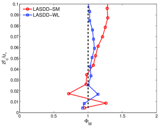
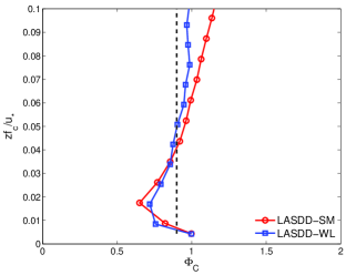
Figure 2: Simulated non-dimensional velocity (left) and scalar (right) gradients. The dashed lines correspond to the values of 1 (left) and 0.9 (right). These values are expected to hold in the surface layer under neutral conditions according to the similarity theory.

In neutrally stratified ABL flows, the observed peak normalized velocity variances occur near the surface and are of the magnitude: $\sigma_{u}^{2}/u_{*}^{2}\sim 5-7$, $\sigma_{v}^{2}/u_{*}^{2}\sim 3-4,$ and $\sigma_{w}^{2}/u_{*}^{2}\sim 1-2$ gran92 . The corresponding values found in our simulations (Figure 3) approximately fall in these ranges. The simulated results also concur with the outer boundary layer observations. For example, the KONTUR data gran86 give $\sigma_{u}^{2}/u_{*}^{2}\sim\sigma_{v}^{2}/u_{*}^{2}\sim 1$ and $\sigma_{w}^{2}/u_{*}^{2}\sim 0.5$ at $z=0.75z_{i}$ (where $z_{i}$ denotes the inversion height). The normalized scalar variances $(\sigma_{c}^{2}/c_{*}^{2})$ are also shown in Figure 3. Here, $c_{*}$ is the surface scalar scale ($=-\overline{wc}_{0}/u_{*}$). In andr94 , it was found that the consensus among different SGS models is poorer in the case of passive scalar in comparison to the momentum case. The disagreements between different SGS models could be partially attributed to different a priori prescriptions for the SGS Prandtl ($Pr_{SGS}$) number, and underscore the need for the determination of $Pr_{SGS}$ in a self-consistent manner, as is done in the present study. One must also acknowledge the facts that the passive scalars exhibit complex spatio-temporal structure, and the statistical and dynamical properties of passive scalars are remarkably different from the underlying velocity fields warh00 ; shra00 .

We point out that the individual plots in Figure 3 represent both the normalized resolved and total (resolved + SGS) variances. In the LASDD modeling approach, one does not solve additional prognostic equations for the SGS turbulence kinetic energy (TKE) and the SGS scalar variances. However, the SGS variances can be roughly diagnosed using the approach of Mason maso89 .

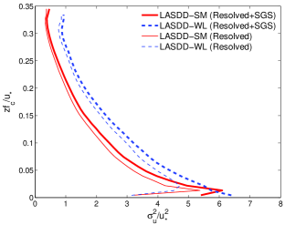
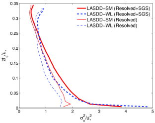
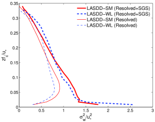
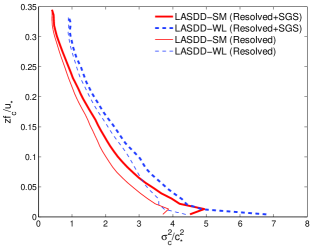
Figure 3: Simulated normalized longitudinal (top-left), transverse (top-right), vertical (bottom-left) velocity variances. Simulated normalized scalar variances are shown in the bottom-right plot.

The one-dimensional longitudinal velocity and passive scalar spectra are computed at heights $z=0.1z_{i}$, and $z=0.5z_{i}$, and presented in Figure 4. The spectra highlight the most important difference between the LASDD-SM and LASDD-WL SGS models: the LASDD-WL SGS model seems to be over-dissipative (indicated by steeper spectral slopes at higher wavenumbers). In the case of the LASDD-SM model, the longitudinal velocity and scalar spectra clearly show extended inertial range ($k_{1}^{-5/3}$ scaling) at $z=0.5z_{i}$ . Near the surface ($z=0.1z_{i}$), the longitudinal velocity spectra show the anticipated production range ($k_{1}^{-1}$), as well as a short inertial range. Recent research suggests that the production range is (likely) related to elongated streaky velocity structures (see below). Traditional SGS models typically do not reproduce well defined inertial ranges in coarse-resolution simulations (cf. andr94 ). From that perspective, the performance of the LASDD models could be considered a near success. We note that the original plane-averaged port00 and the Lagrangian-averaged bouz05 ; stol06 scale-dependent dynamic SGS models also reproduced the characteristics of the one-dimensional longitudinal velocity spectra remarkably well. However, near the surface, the passive scalar spectra predicted by these SGS models showed unphysical pile up of scalar variances port04 ; stol06 . This was possibly due to small dynamically determined eddy-diffusion coefficients near the surface port04 ; stol06 . In the present study we did not encounter this issue.

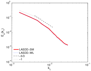
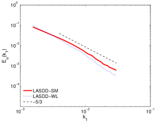
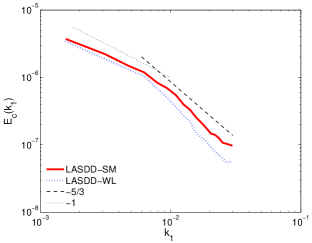
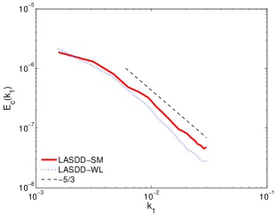
Figure 4: Spectra of longitudinal velocity (top), and passive scalar (bottom). The spectra are plotted for $z=0.1z_{i}$ (left), and $z=0.5z_{i}$ (right) levels. The dashed and dotted lines depict the inertial range $(k_{1}^{-5/3})$ and production range $(k_{1}^{-1})$ scalings, respectively.

A few previous LES studies have reported the existence of elongated streaky structures in the neutral surface layers koso97 ; sull94 ; maso87 ; moen94 ; ding01 ; carl02 . The link between experimentally observed long production range ($k^{-1}$ scaling) in the streamwise spectra of the longitudinal velocity and the elongated streaky structures has recently been discussed in depth by Carlotti carl02 . Moreover, strong correlations between these streaky structures and large negative momentum flux were earlier reported by moen94 . From Figure 5 (top), it is clear that both the LASDD models show streaky structures, roughly parallel to the mean wind direction, in the surface layer (at $z=0.1z_{i}$). However, significant morphologic differences are noticeable in the mid-ABL flow structures. In accordance with past studies (cf. moen94 ), the LASDD-SM SGS model predicts non-coherent structures at $z=0.5z_{i}$. In contrast, large coherent structures persist in the LASDD-WL model results (Figure 5, bottom-right). Another interesting feature of this plot is the (virtual) non-existence of fine-scale flow structures. This can be directly associated with the over-dissipative nature of the LASDD-WL SGS model, as discussed before. In essence, we can infer that the (non-)existence of coherent structures in NBL flows are strongly dependent on SGS parameterizations, especially for coarse-resolution simulations. A few previous studies somewhat support this inference. For instance, the nonlinear SGS model koso97 , and the modified Smagorinsky SGS model ding01 barely produced any elongated streaky structures.

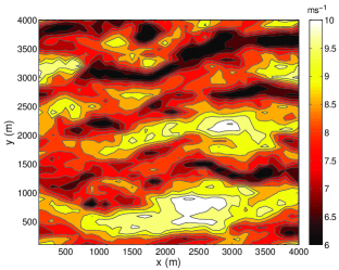
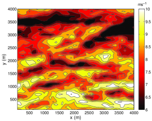
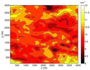
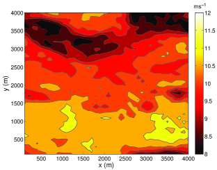
Figure 5: Visualization of longitudinal velocity fields simulated by LASDD-SM (left), and LASDD-WL (right) SGS models. The horizontal cross-sections are taken at $z=0.1z_{i}$ (top), and $z=0.5z_{i}$ (bottom).

4 Concluding Remarks

Two locally averaged scale-dependent dynamic SGS closures – the LASDD-SM basu06a ; basu06b and the LASDD-WL (this study) – have been used to simulate a neutral ABL case. Although the theoretical foundations of these SGS models are fundamentally different, results presented in Figures 1 through 5 illustrate strong congruence between their results, and with firmly established results (i.e. the Monin-Obukhov similarity theory and the inertial range scaling of spectra). The normalized variances computed in our simulations also closely follow the ones calculated from field measurements. The major noticeable and consistent difference between the results is shown in Figure 4: the LASDD-WL SGS model appears to be over-dissipative at the higher wavenumbers, in comparison to the LASDD-SM SGS model. In Figure 5, we see that both SGS models predict elongated streaky structures in the near-wall region ($z=0.1z_{i}$). These coherent structures are no longer evident at higher locations in the domain, in the case of the LASDD-SM SGS model-based simulation. Due to undue dissipation, the LASDD-WL SGS model-based simulation results in quite different flow structures at this level.

The Wong-Lilly SGS base model requires fewer assumptions and comes at slightly less computational cost in comparison to the commonly used Smagorinsky SGS base model. Unfortunately, these advantages seem to be offset by its over-dissipative tendency at higher wavenumbers. Some inherent assumptions of the Smagorinsky base model can also be eliminated by solving a prognostic equation for the TKE. However, when using this TKE SGS approach, the SGS model coefficients are often tuned for different ABL flow conditions sull94 ; sull03 . An alternative approach would be to formulate a dynamic version of the TKE SGS model, which will also account for energy backscatter. We are currently working on this SGS approach to better represent the physics of atmospheric boundary layer flows.

Appendix

The SGS model proposed by Wong and Lilly wong94 can be written as:

$$\tau_{ij}-\frac{1}{3}\tau_{kk}\delta_{ij}=-2C_{WL}\Delta_{f}^{4/3}\tilde{S}_{ij}$$ (A1)

where $\tau_{ij}$ and $\tilde{S}_{ij}$ denote the SGS stress tensor and the resolved strain rate tensor, respectively. $C_{WL}$ is a model coefficient to be specified or determined dynamically. In a recent LES study of neutral boundary layer flows, Chow et al. chow05 utilized a dynamic version of this SGS model in conjunction with the approximate deconvolution model (ADM) for resolvable subfilter-scale (RSFS) components. To account for the smaller underresolved eddies in the surface layer, they used a near-wall stress model in addition to the dynamic Wong-Lilly SGS and ADM-RSFS models. As an alternative approach, in this work, we formulate a locally averaged scale-dependent dynamic version of Equation (A1) (named LASDD-WL).

The SGS stress tensor ($\tau_{ij}$) at the filter scale ($\Delta_{f}$) is defined as: $\tau_{ij}=\widetilde{u_{i}u_{j}}-\widetilde{u_{i}}\widetilde{u_{j}}$. In a seminal work, Germano et al. germ91 proposed to invoke an additional explicit test filter of width $\alpha\Delta_{f}$ in order to dynamically compute the SGS coefficients. Consecutive filtering at scales $\Delta_{f}$ and at $\alpha\Delta_{f}$ leads to a SGS turbulent stress tensor ($T_{ij}$) at the test filter scale $\alpha\Delta_{f}$:

$$T_{ij}=\overline{\widetilde{u_{i}~{}u_{j}}}-\overline{\widetilde{u}_{i}}~{}\overline{\widetilde{u}_{j}},$$ (A2)

where an overline $\overline{(\cdots)}$ denotes filtering at a scale of $\alpha\Delta_{f}$. From the definitions of $\tau_{ij}$ and $T_{ij}$ an algebraic relation can be formed, known in the literature as the Germano identity:

$$L_{ij}=\overline{\widetilde{u}_{i}\widetilde{u}_{j}}-\overline{\widetilde{u}_{i}}~{}\overline{\widetilde{u}_{j}}=T_{ij}-\overline{\tau_{ij}}.$$ (A3)

This identity is then effectively used to dynamically obtain unknown SGS model coefficients. In the case of the Wong-Lilly model (Equation (A1)), this identity yields:

$$L_{ij}-\frac{1}{3}L_{kk}\delta_{ij}=\left(C_{WL}\right)_{\Delta_{f}}M_{ij},$$ (A4)

where $M_{ij}=2\Delta_{f}^{4/3}\left(1-\alpha^{4/3}\frac{\left(C_{WL}\right)_{\alpha\Delta_{f}}}{\left(C_{WL}\right)_{\Delta_{f}}}\right)\overline{\widetilde{S_{ij}}}$. If one assumes scale invariance, i.e., $\left(C_{WL}\right)_{\alpha\Delta_{f}}=\left(C_{WL}\right)_{\Delta_{f}}$, then the unknown coefficient $\left(C_{WL}\right)_{\Delta_{f}}$ can be easily determined following the error minimization approach of Lilly lill92 :

$$\left(C_{WL}\right)_{\Delta_{f}}=\frac{\langle L_{ij}M_{ij}\rangle}{\langle M_{ij}M_{ij}\rangle}.$$ (A5)

In the context of the present study, the angular brackets $\langle\cdots\rangle$ denote localized spatial averaging on horizontal planes with a stencil of three by three grid points basu06a ; basu06b .

Recent studies have shown that the assumption of scale invariance is seriously flawed for sheared and stratified boundary layer flows port00 ; port04 ; basu06a ; basu06b ; bouz05 ; stol06 . In other words, the ratio of $\left(C_{WL}\right)_{\alpha\Delta_{f}}$ to $\left(C_{WL}\right)_{\Delta_{f}}$ should not be assumed equal to one for most of these ABL flow scenarios. Rather, this scale-dependence ratio should be determined dynamically. In order to implement the scale-dependent dynamic procedure, one needs to employ a second test filtering operation at a scale of $\alpha^{2}\Delta_{f}$ [denoted by $\widehat{(\cdots)}$]. Invoking the Germano identity for the second time leads to:

$$Q_{ij}-\frac{1}{3}Q_{kk}\delta_{ij}=\left(C_{WL}\right)_{\Delta_{f}}N_{ij},$$ (A6)

where

$$Q_{ij}=\widehat{\widetilde{u_{i}}\widetilde{u_{j}}}-\widehat{\widetilde{u_{i}}}\widehat{\widetilde{u_{j}}}$$

and

$$N_{ij}=2\Delta_{f}^{4/3}\left(1-\alpha^{8/3}\frac{\left(C_{WL}\right)_{\alpha^{2}\Delta_{f}}}{\left(C_{WL}\right)_{\Delta_{f}}}\right)\widehat{\widetilde{S_{ij}}}.$$

This results in:

$$\left(C_{WL}\right)_{\Delta_{f}}=\frac{\langle Q_{ij}N_{ij}\rangle}{\langle N_{ij}N_{ij}\rangle}.$$ (A7)

Following port00 , the following scale-dependence assumption can be made:

$$\beta=\frac{\left(C_{WL}\right)_{\alpha\Delta_{f}}}{\left(C_{WL}\right)_{\Delta_{f}}}=\frac{\left(C_{WL}\right)_{\alpha^{2}\Delta_{f}}}{\left(C_{WL}\right)_{\alpha\Delta_{f}}},$$ (A8)

This is a much weaker assumption than the scale-invariance modeling assumption of $\beta=1$. Now, from Equations (A5) and (A7), using Equation (A8), one solves for the unknown parameter $\beta$, which in turn is used to compute the Wong-Lilly SGS model coefficient, $\left(C_{WL}\right)_{\Delta_{f}}$, utilizing Equation (A5).

Solving for $\beta$ essentially involves finding the roots of a fifth-order polynomial port00 :

$$A_{0}+A_{1}\beta+A_{2}\beta^{2}+A_{3}\beta^{3}+A_{4}\beta^{4}+A_{5}\beta^{5}=0$$ (A9)

where $A_{0}=a_{1}a_{3}-a_{6}a_{8}$, $A_{1}=a_{1}a_{4}-a_{7}a_{8}$, $A_{2}=a_{2}a_{3}+a_{1}a_{5}-a_{6}a_{9}$, $A_{3}=a_{2}a_{4}-a_{7}a_{9}$, $A_{4}=a_{2}a_{5}-a_{6}a_{10}$, and $A_{5}=-a_{7}a_{10}$. In the case of Wong-Lilly SGS base model, we derive: $a_{1}=\langle Q_{ij}\widehat{\widetilde{S_{ij}}}\rangle$, $a_{2}=\langle-\alpha^{8/3}Q_{ij}\widehat{\widetilde{S_{ij}}}\rangle$, $a_{3}=\langle{\overline{\widetilde{S_{ij}}}}^{2}\rangle$, $a_{4}=\langle-2\alpha^{4/3}{\overline{\widetilde{S_{ij}}}}^{2}\rangle$, $a_{5}=\langle\alpha^{8/3}{\overline{\widetilde{S_{ij}}}}^{2}\rangle$, $a_{6}=\langle L_{ij}{\overline{\widetilde{S_{ij}}}}\rangle$, $a_{7}=\langle-\alpha^{4/3}L_{ij}{\overline{\widetilde{S_{ij}}}}\rangle$, $a_{8}=\langle{\widehat{\widetilde{S_{ij}}}}^{2}\rangle$, $a_{9}=\langle-2\alpha^{8/3}{\widehat{\widetilde{S_{ij}}}}^{2}\rangle$, and $a_{10}=\langle\alpha^{16/3}{\widehat{\widetilde{S_{ij}}}}^{2}\rangle$. Please note that the coefficients ($a_{1}$ to $a_{10}$) involve significantly lesser number of tensor terms in comparison to the ones derived by Porté-Agel et al. port00 using the Smagorinsky SGS base model. Lesser number of calculations (specifically the tensor multiplications) undoubtedly lead to cheaper computational costs.

Scale-dependent formulation for scalars can be derived in a similar manner port04 . The Wong-Lilly model for a generic scalar ($c$) could be written as:

$$q_{i}=-\frac{C_{WL}}{Pr_{SGS}}\Delta_{f}^{4/3}\frac{\partial\tilde{c}}{\partial x_{i}}$$ (A10)

where $Pr_{SGS}$ is the so-called SGS Prandtl number. In the dynamic or scale-dependent dynamic modeling approaches, typically the lumped SGS coefficient ($C_{WL}Pr_{SGS}^{-1}$) is determined in a self-consistent manner. This procedure not only eliminates the need for any ad hoc assumption about the SGS Prandtl number ($Pr_{SGS}$), it also completely decouples the SGS scalar flux estimation from SGS stress computation. In the scale-dependent approach port04 , one further defines a scale-dependent parameter for scalars ($\beta_{c}$), analogous to Equation (A8). For the Wong-Lilly SGS base model, it could be written as:

$$\beta_{c}=\frac{\left(C_{WL}Pr_{SGS}^{-1}\right)_{\alpha\Delta_{f}}}{\left(C_{WL}Pr_{SGS}^{-1}\right)_{\Delta_{f}}}=\frac{\left(C_{WL}Pr_{SGS}^{-1}\right)_{\alpha^{2}\Delta_{f}}}{\left(C_{WL}Pr_{SGS}^{-1}\right)_{\alpha\Delta_{f}}},$$ (A11)

As before, $\beta_{c}$ could be determined by solving the fifth-order polynomial:

$$A_{0}+A_{1}\beta_{c}+A_{2}\beta_{c}^{2}+A_{3}\beta_{c}^{3}+A_{4}\beta_{c}^{4}+A_{5}\beta_{c}^{5}=0$$ (A12)

where $A_{0}=a_{1}a_{3}-a_{6}a_{8}$, $A_{1}=a_{1}a_{4}-a_{7}a_{8}$, $A_{2}=a_{2}a_{3}+a_{1}a_{5}-a_{6}a_{9}$, $A_{3}=a_{2}a_{4}-a_{7}a_{9}$, $A_{4}=a_{2}a_{5}-a_{6}a_{10}$, and $A_{5}=-a_{7}a_{10}$. For the Wong-Lilly SGS base model for scalars, we get: $a_{1}=\langle K_{i}^{\prime}\widehat{\frac{\partial\widetilde{c}}{\partial x_{i}}}\rangle$, $a_{2}=\langle-\alpha^{8/3}K_{i}^{\prime}\widehat{\frac{\partial\widetilde{c}}{\partial x_{i}}}\rangle$, $a_{3}=\langle{\overline{\frac{\partial\widetilde{c}}{\partial x_{i}}}}^{2}\rangle$, $a_{4}=\langle-2\alpha^{4/3}{\overline{\frac{\partial\widetilde{c}}{\partial x_{i}}}}^{2}\rangle$, $a_{5}=\langle\alpha^{8/3}{\overline{\frac{\partial\widetilde{c}}{\partial x_{i}}}}^{2}\rangle$, $a_{6}=\langle K_{i}\overline{\frac{\partial\widetilde{c}}{\partial x_{i}}}\rangle$, $a_{7}=\langle-\alpha^{4/3}K_{i}\overline{\frac{\partial\widetilde{c}}{\partial x_{i}}}\rangle$, $a_{8}=\langle{\widehat{\frac{\partial\widetilde{c}}{\partial x_{i}}}}^{2}\rangle$, $a_{9}=\langle-2\alpha^{8/3}{\widehat{\frac{\partial\widetilde{c}}{\partial x_{i}}}}^{2}\rangle$, and $a_{10}=\langle\alpha^{16/3}{\widehat{\frac{\partial\widetilde{c}}{\partial x_{i}}}}^{2}\rangle$. Here, $K_{i}=\left(\overline{\widetilde{u_{i}}\widetilde{c}}-\overline{\widetilde{u_{i}}}~{}\overline{\widetilde{c}}\right)$, and $K_{i}^{\prime}=\left(\widehat{\widetilde{u_{i}}\widetilde{c}}-\widehat{\widetilde{u_{i}}}~{}\widehat{\widetilde{c}}\right)$.

References

- (1) Germano, M., Piomelli, U., Moin, P. and Cabot, W. H.: 1991, A dynamic subgrid-scale eddy viscosity model, Phys. Fluids A 3, 1760–1765.
- (2) Pope, S. B.: 2004, Ten questions concerning the large-eddy simulation of turbulent flows, New J. Phys. 6, 1–24.
- (3) Meyers, J., Geurts, B. J. and Baelmans, M.: 2005, Optimality of the dynamic procedure for large-eddy simulations, Phys. Fluids 17, 045108.
- (4) Porté-Agel, F., Meneveau, C. and Parlange, M. B.: 2000, A scale-dependent dynamic model for large-eddy simulation: application to a neutral atmospheric boundary layer, J. Fluid Mech. 415, 261–284.
- (5) Porté-Agel, F.: 2004, A scale-dependent dynamic model for scalar transport in LES of the atmospheric boundary layer, Boundary-Layer Meteorol. 112, 81-105.
- (6) Basu, S. and Porté-Agel, F.: 2006, Large-eddy simulation of stably stratified atmospheric boundary layer turbulence: a scale-dependent dynamic modeling approach, J. Atmos. Sci. 63, 2074–2091.
- (7) Basu, S., Porté-Agel, F., Foufoula-Georgiou, E., Vinuesa, J.-F. and Pahlow, M.: 2006, Revisiting the local scaling hypothesis in stably stratified atmospheric boundary layer turbulence: an integration of field and laboratory measurements with large-eddy simulations, Boundary-Layer Meteorol. 10.1007/s10546-005-9036-2.
- (8) Bou-zeid, E., Meneveau, C. and Parlange, M.: 2006, A scale-dependent Lagrangian dynamic model for large eddy simulation of complex turbulent flows, Phys. Fluids 17, 025105.
- (9) Stoll, R. and Porté-Agel, F.: 2006, Dynamic subgrid-scale models for momentum and scalar fluxes in large-eddy simulations of neutrally stratified atmospheric boundary layers over heterogeneous terrain, Water Resour. Res. 42, W01409.
- (10) Smagorinsky, J.: 1963, General Circulation Experiments with the Primitive Equations, Mon. Weath. Rev. 91, 99–164.
- (11) Wong, V. and Lilly, D.: 1994, A comparison of two dynamic subgrid scale closure methods for turbulent thermal convection, Phys. Fluids 6, 1016–1023.
- (12) Andrén, A., Brown, A. R., Graf, J., Mason, P. J., Moeng, C.-H., Nieuwstadt, F. T. M. and Schumann, U.: 1994, Large-eddy simulation of a neutrally stratified boundary layer: a comparison of four codes, Q. J. Royal Meteorol. Soc. 120, 1457–1484.
- (13) Kosović, B.: 1997, Subgrid-scale modelling for the large-eddy simulation of high-Reynolds-number boundary layers, J. Fluid Mech. 336, 151–182.
- (14) Chow, F. K., Street, R. L., Xue, M. and Ferziger, J. H.: 2005, Explicit filtering and reconstruction turbulence modeling for large-eddy simulation of neutral boundary layer flow, J. Atmos. Sci. 62, 2058–2077.
- (15) Mason, P. J. and Thomson, D. J.: 1992, Stochastic backscatter in large-eddy simulations of boundary layers, J. Fluid Mech. 242, 51–78.
- (16) Sullivan, P. P., McWilliams, J. C. and Moeng, C.-H.: 1994, A subgrid-scale model for large-eddy simulation of planetary boundary-layer flows, Boundary-Layer Meteorol. 71, 247–276.
- (17) Esau, I.: 2004, Simulation of Ekman boundary layers by large eddy model with dynamic mixed subfilter closure, Environ. Fluid Mech. 4, 273–303.
- (18) Businger, J. A., Wyngaard, J. C., Izumi, Y. and Bradley, E. F.: 1971, Flux-profile relationships in the atmospheric surface layer, J. Atmos. Sci. 28, 181–189.
- (19) Kader, B. A. and Yaglom, A. M.: 1990, Mean field and fluctuation moments in unstably stratified turbulent boundary layers, J. Fluid Mech. 212, 637–662.
- (20) Grant, A. L. M.: 1992, The structure of turbulence in the near-neutral atmospheric boundary layer, J. Atmos. Sci. 49, 226–239.
- (21) Grant, A. L. M.: 1986, Observations of boundary layer structure made during the KONTUR experiment, Q. J. Royal Meteorol. Soc. 112, 825–841.
- (22) Warhaft, Z.: 2000, Passive scalars in turbulent flows, Annu. Rev. Fluid Mech. 32, 203–240.
- (23) Shraiman, B. I. and Siggia, E. D.: 2000, Scalar turbulence, Nature 405, 639–646.
- (24) Mason, P.: 1989, Large-eddy simulation of the convective atmospheric boundary layer, J. Atmos. Sci. 46, 1492–1516.
- (25) Mason, P. J. and Thomson, D. J.: 1987, Large-eddy simulations of the neutral-static-stability planetary boundary layer, Quart. J. Roy. Meteorol. Soc. 113, 413–443.
- (26) Moeng, C.-H. and Sullivan, P. P.: 1994, A comparison of shear- and buoyancy-driven planetary boundary layer flows, J. Atmos. Sci. 51, 999–1022.
- (27) Ding, F., Arya, S. P. and Lin, Y.-L.: 2001, Large-eddy simulations of the atmospheric boundary layer using a new subgrid-scale model. Part I: Slightly unstable and neutral cases, Environ. Fluid Mech. 1, 29–47.
- (28) Carlotti, P.: 2002, Two-point properties of atmospheric turbulence very close to the ground: Comparison of a high resolution LES with theoretical models, Boundary-Layer Meteorol. 104, 381–410.
- (29) Sullivan, P. P., Horst, T. W., Lenschow, D. H., Moeng, C.-H. and Weil, J. C.: 2003, Structure of subfilter-scale fluxes in the atmospheric surface layer with application to large-eddy simulation modelling, J. Fluid Mech. 482, 101–139.
- (30) Lilly, D. K.: 1992, A proposed modification of the Germano subgridscale closure method, Phys. Fluids A 4, 633–635.