Photoionization effects in streamer discharges

Abstract

In this paper we study the effects of photoionization processes on the propagation of both negative and positive streamer discharges. We show that negative fronts accelerate in the presence of photoionization events. The appearance and propagation of positive streamers travelling with constant velocity is explained as the result of the combined effects of photoionization and electron diffusion. The photoionization range plays an important role for the selection of the velocity of the streamer as we show in this work.

I Introduction

Since Raether Raether used cloud chamber photographs to study the creation and propagation of streamer discharges there has been considerable effort to understand the underlying processes driving them. A streamer discharge is considered to be a plasma channel which propagates in a gas. The discharge propagates by ionizing the medium in front of its charged head due to a strong field induced by the head itself. This kind of discharges produces sharp ionization waves that propagate into a non-ionized gas, leaving a non-equilibrium plasma behind.

Raether himself realized that Townsend’s mechanism which takes into account the creation of extra charge by impact ionization Loeb was not enough to explain the velocity of propagation of a streamer discharge. He pointed to photoionization as the process which enhances the propagation of the streamer. Due to the recombination of positive ions and electrons, the head of the discharge is a strong source of high energetic photons. Photons, emitted by the atoms that previous collisions have excited, initiate secondary avalanches in the vicinity of the head which move driven by the local electric field increasing the velocity of propagation of the front.

In this paper we study the role played by photoionization in the propagation of both negative and positive streamers. We take a model widely used in numerical simulations and find an effective simplified model. We discuss how this simplified model retains all the physics of streamer discharges including photoionization. The photoionization is modelled as a nonlocal source term. We take the case of air and consider optical emissions from N₂ and N${}_{2}^{+}$ molecules. Then we consider the sole role of photoionization in negative planar shock fronts. Finally we analyse the case of positive planar fronts and propose a mechanism for their formation and propagation. We end with an analysis of results and conclusions.

II Model for a streamer discharge

Here we consider a fluid description of a low-ionized plasma based on kinetic theory. The balance equation for the particle density of electrons $N_{e}$ is the lowest moment of the Boltzmann equation,

$$\frac{\partial N_{e}}{\partial\tau}+\nabla_{\bf R}\cdot\left(N_{e}{\bf U}_{e}\right)=S_{e},$$ (1)

where ${\bf R}$ is the position vector, $\tau$ is time, $\nabla_{\bf R}$ is the gradient in configuration space, ${\bf U}_{e}({\bf R},\tau)$ is the average (fluid) velocity of electrons and $S_{e}$ is the source term, i.e. the net creation rate of electrons per unit volume as a result of collisions. It is convenient to define the electron current density ${\bf J}_{e}({\bf R},\tau)$ as

$${\bf J}_{e}({\bf R},\tau)=N_{e}({\bf R},\tau)\,{\bf U}_{e}({\bf R},\tau),$$ (2)

so that the balance equation can also be written as

$$\frac{\partial N_{e}}{\partial\tau}+\nabla_{\bf R}\cdot{\bf J}_{e}=S_{e}.$$ (3)

The same procedure can be done, in principle, for positive ($N_{p}$) and negative ($N_{n}$) ion densities to give

$$\frac{\partial N_{p}}{\partial\tau}+\nabla_{\bf R}\cdot{\bf J}_{p}=S_{p},$$ (4)

$$\frac{\partial N_{n}}{\partial\tau}+\nabla_{\bf R}\cdot{\bf J}_{n}=S_{n},$$ (5)

where ${\bf J}_{p,n}$ are the current densities of positive and negative ions, respectively, and $S_{p,n}$ are source terms. Conservation of charge has to be imposed in all processes, so that the condition

$$S_{p}=S_{e}+S_{n},$$ (6)

holds for the source terms. Some physical approximations can now be done in order to simplify the balance equations (3)–(5). The first one is to assume that the electron current ${\bf J}_{e}$ is approximated as the sum of a drift (electric force) and a diffusion term

$${\bf J}_{e}=-\mu_{e}{\boldsymbol{\cal E}}N_{e}-D_{e}\nabla_{\bf R}N_{e},$$ (7)

where ${\boldsymbol{\cal E}}$ is the total electric field (the sum of the external electric field applied to initiate the propagation of a ionization wave and the electric field created by the local point charges) and $\mu_{e}$ and $D_{e}$ are the mobility and diffusion coefficient of the electrons. Note that, as the initial charge density is low and there is no applied magnetic field, the magnetic effects in equation (7) are neglected. Concerning the diffusion coefficient, in the case of equilibrium, the kinetic theory of gases links diffusion to mobility through Einstein’s relation $D_{e}/\mu_{e}=kT/e$. With respect to positive and negative ions, on time-scales of interest for the case of streamer discharges, the ion currents can be neglected because they are more than two orders of magnitude smaller than the electron ones AJP , so we will take

$${\bf J}_{p}={\bf J}_{n}=0.$$ (8)

Consider now the processes that give rise to the source terms $S_{e,p,n}$:

1. The first of these processes is the creation of free electrons by impact ionization: an electron is accelerated in a strong local field, collides with a neutral molecule and ionizes it. The result is the generation of new free electrons and a positive ion. The ionization rate is given by

   $$S_{e}^{i}=S_{p}^{i}=\nu_{i}N_{e},$$ (9)

   where the ion production rate $\nu_{i}$ depends on the local electric field, the density of the neutral particles of the gas and their effective ionization cross sections.

2. The second possible process is attachment: when an electron collides with a neutral gas atom or molecule, it may become attached, forming a negative ion. This process depends on the energy of the electron and the nature of the gas Dhali . The attachment rate can be written as

   $$S_{n}^{a}=-S_{e}^{a}=\nu_{a}N_{e},$$ (10)

   where $\nu_{a}$ is the attachment rate coefficient. Note that the creation of negative ions due to these processes reduces the number of free electrons, so $S_{e}^{a}$ is negative.

3. There are also two possible kinds of recombination processes: a free electron with a positive ion and a negative ion with a positive ion. The recombination rate is

   $$S_{e}^{ep}=S_{p}^{ep}=-\nu_{ep}N_{e}N_{p},$$ (11)

   for electron-positive ion recombination, and

   $$S_{p}^{np}=S_{n}^{np}=-\nu_{np}N_{n}N_{p},$$ (12)

   for positive ion-negative ion recombination, $\nu_{ep}$ and $\nu_{np}$ being the recombination coefficients respectively.

4. Finally, we can include photoionization: photons created by recombination or scattering processes can interact with a neutral atom or molecule, producing a free electron and a positive ion. Models for the creation rate of electron-positive ion pairs due to photoionization are non-local. This rate will be here denoted by

   $$S_{e}^{ph}=S_{p}^{ph}=S^{ph}.$$ (13)

Taking into account the expressions (7) and (8) for the current densities, and the equations (9)–(13) for the source terms, we obtain a deterministic model for the evolution of the streamer discharge,

$$\frac{\partial N_{e}}{\partial\tau} = \nabla_{\bf R}\cdot\left(\mu_{e}{\boldsymbol{\cal E}}N_{e}+D_{e}\nabla_{\bf R}N_{e}\right)+\nu_{i}N_{e}$$ (14)

$$- \nu_{a}N_{e}-\nu_{ep}N_{e}N_{p}+S^{ph},$$

$$\frac{\partial N_{p}}{\partial\tau} = \nu_{i}N_{e}-\nu_{ep}N_{e}N_{p}-\nu_{np}N_{n}N_{p}+S^{ph},$$ (15)

$$\frac{\partial N_{n}}{\partial\tau} = \nu_{a}N_{e}-\nu_{np}N_{n}N_{p}.$$ (16)

In order for the model to be complete, it is necessary to give expressions for the source coefficients $\nu$, the electron mobility $\mu_{e}$, the diffusion coefficient $D_{e}$ and the photoionization source term $S^{ph}$. Finally, we have to impose equations for the evolution of the electric field ${\boldsymbol{\cal E}}$. This evolution of the electric field is given by Poisson’s equation,

$$\nabla_{\bf R}\cdot{\boldsymbol{\cal E}}=\frac{e}{\varepsilon_{0}}\,\left(N_{p}-N_{n}-N_{e}\right),$$ (17)

where $e$ is the absolute value of the electron charge, $\varepsilon_{0}$ is the permittivity of the gas, and we are assuming that the absolute value of the charge of positive and negative ions is $e$. Note that the coupling between the space charges and the electric field in the model makes the problem nonlinear. The model given by (14), (15), and (16), together with (17) has been studied numerically in the literature liu . There are other works where the electrical current due to ions (8) is taken into account although not photoionization Vit .

III A simplified model

In this section we will simplify the model given by equations (14)–(16). In order to be specific and fix ideas we shall consider the case of air. In liu , some data are presented for the ionization coefficients and the photoionization source term. Using these data we shall see that one can neglect the quadratic terms involving the coefficients $\nu_{ep}$ and $\nu_{np}$ since they are about two orders of magnitude smaller than $\nu_{i}$. The same can be said about the terms involving the coefficient $\nu_{a}$. First we write equations (14)–(16) as

$$\frac{\partial N_{e}}{\partial\tau} = \nabla_{\bf R}\cdot\left(\mu_{e}{\boldsymbol{\cal E}}N_{e}+D_{e}\nabla_{\bf R}N_{e}\right)$$ (18)

$$+ \left(\nu_{i}-\nu_{a}-\nu_{ep}N_{p}\right)N_{e}+S^{ph},$$

$$\frac{\partial N_{p}}{\partial\tau} = \left(\nu_{i}-\nu_{ep}N_{p}\right)N_{e}-\nu_{np}N_{n}N_{p}+S^{ph},$$ (19)

$$\frac{\partial N_{n}}{\partial\tau} = \nu_{a}N_{e}-\nu_{np}N_{n}N_{p}.$$ (20)

In these equations, and using the data in liu (Figure 1 and Table 2), the term $\nu_{i}$ is of the order of $10^{10}\,\mbox{s}^{-1}$ for large electric fields, $\nu_{a}$ is about $10^{8}\,\mbox{s}^{-1}$, and $\nu_{ep}$ and $\nu_{np}$ are about $10^{-13}\,\mbox{m}^{3}\cdot\mbox{s}^{-1}$. Moreover, $N_{p}$ is of the same order of $N_{e}$. Then, in equation (20), in the stationary regime when the particle densities reach the saturation values, one has $N_{n}\sim\nu_{a}/\nu_{np}\sim 10^{21}\mbox{m}^{-3}$. So that, it follows from equation (19) that, in the stationary regime, the term $\nu_{np}N_{n}N_{p}\sim 10^{8}N_{p}$ is two orders of magnitude smaller than the term $\nu_{i}N_{e}\sim 10^{10}N_{e}$. Hence the terms $\nu_{a}N_{e}$ and $\nu_{np}N_{n}N_{p}$ can safely be neglected. The model then reads

$$\frac{\partial N_{e}}{\partial\tau} = \nabla_{\bf R}\cdot\left(\mu_{e}{\boldsymbol{\cal E}}N_{e}+D_{e}\nabla_{\bf R}N_{e}\right)$$ (21)

$$+ \left(\nu_{i}-\nu_{ep}N_{p}\right)N_{e}+S^{ph},$$

$$\frac{\partial N_{p}}{\partial\tau} = \left(\nu_{i}-\nu_{ep}N_{p}\right)N_{e}+S^{ph}.$$ (22)

In order to neglect the term $\nu_{ep}N_{e}N_{p}$ by comparison with the term $\nu_{i}N_{e}$, it is necessary than $N_{p}$ (and then $N_{e}$) satisfies $N_{p}\ll\nu_{i}/\nu_{ep}\sim 10^{23}\mbox{m}^{-3}$. To see that it is the case, we use the Poisson equation (17) to write equation (21), without the term $\nu_{ep}N_{e}N_{p}$, as

$$\frac{\partial N_{e}}{\partial\tau} - \mu_{e}{\boldsymbol{\cal E}}\cdot\nabla_{\bf R}N_{e}-D_{e}\nabla_{\bf R}^{2}N_{e}$$ (23)

$$= \left(\nu_{i}+\mu_{e}\frac{e}{\varepsilon_{0}}\left(N_{p}-N_{e}\right)\right)N_{e}+S^{ph}.$$

From this expression, looking at its RHS, we can see that, while $S^{ph}$ has small effect and the total populations of both ions and electrons, $N_{e}$ can grow only up to a saturation value at which $\nu_{i}+\mu_{e}\frac{e}{\varepsilon_{0}}\left(N_{p}-N_{e}\right)=0$, i.e.

$$N_{e}-N_{p}\leq\frac{\nu_{i}}{\mu_{e}e/\varepsilon_{0}}\sim 10^{20}\mbox{m}^{3},$$ (24)

at all times. Therefore neither $N_{p}$ nor $N_{e}$ reach values close to $10^{23}\mbox{m}^{-3}$, and all the assumptions which led to neglect $\nu_{ep}N_{e}N_{p}$ are justified. Our simplified model will be

$$\frac{\partial N_{e}}{\partial\tau} = \nabla_{\bf R}\cdot\left(\mu_{e}{\boldsymbol{\cal E}}N_{e}+D_{e}\nabla_{\bf R}N_{e}\right)+\nu_{i}N_{e}+S^{ph},$$ (25)

$$\frac{\partial N_{p}}{\partial\tau} = \nu_{i}N_{e}+S^{ph}.$$ (26)

Let us remark that the orders of magnitude deduced for $N_{e}$ and $N_{p}$ coincide with those found in full numerical simulations by Liu and Pasko liu .

IV The photoionization term

In this section we will write down an explicit form of the photoionization source term. In our study on the effects of photoionization on the evolution of streamers in air we consider that only optical emissions from ${\mbox{N}}_{2}$ and ${\mbox{N}}_{2}^{+}$ molecules can ionize ${\mbox{O}}_{2}$ molecules. The photoionization rate, due to the fact that the number of photons emitted is physically proportional to the number of ions produced by impact ionization, is written as the following nonlocal source term liu ; naidis ,

$$S_{ph}({\bf R})=S_{0}\int\nu_{i}({\bf R}^{\prime})N_{e}({\bf R}^{\prime})\,K_{ph}(|{\bf R}-{\bf R}^{\prime}|)\,d^{3}R^{\prime},$$ (27)

where $S_{0}$ is given by

$$S_{0}=\frac{1}{4\pi}\frac{p_{q}}{p+p_{q}}\,\xi\left(\frac{\nu_{*}}{\nu_{i}}\right)\frac{1}{\ln{(\chi_{max}/\chi_{min})}}.$$ (28)

In this expression, $p_{q}$ is the quenching pressure of the single states of ${\mbox{N}}_{2}$, $p$ is the gas pressure, $\xi$ is the average photoionization efficiency in the interval of radiation frequencies relevant to the problem, $\nu_{*}$ is the effective excitation coefficient for ${\mbox{N}}_{2}$ state transitions from which the ionization radiation comes out (we take $\nu_{*}/\nu_{i}$ to be a constant), and $\chi_{min}$ and $\chi_{max}$ are, respectively, the minimum and maximum absorption cross sections of ${\mbox{O}}_{2}$ in the relevant radiation frequency interval. The kernel $K_{ph}(|{\bf R}-{\bf R}^{\prime}|)$ is written as Zhe

$$K_{ph}(R)=\frac{\exp{(-\chi_{1}R)}-\exp{(-\chi_{2}R)}}{R^{3}},$$ (29)

in which $\chi_{1}=\chi_{min}p_{O_{2}}$ and $\chi_{2}=\chi_{max}p_{O_{2}}$, so that $\chi_{1}<\chi_{2}$. For the ionization coefficient $\nu_{i}$, we take the phenomenological approximation given by Townsend Loeb ,

$$\nu_{i}=\mu_{e}|{\boldsymbol{\cal E}}|\alpha_{0}\exp\left(\frac{-{\cal E}_{0}}{|{\boldsymbol{\cal E}}|}\right),$$ (30)

where $\mu_{e}$ is the electron mobility, $\alpha_{0}$ is the inverse of ionization length, and ${\cal E}_{0}$ is the characteristic impact ionization electric field. Note also that $\mu_{e}|{\boldsymbol{\cal E}}|$ is the drift velocity of electrons. Townsend approximation provides some physical scales and intrinsic parameters of the model. It is then convenient to reduce the equations to dimensionless form. Natural units are given by the ionization length $R_{0}=\alpha_{0}^{-1}$, the characteristic impact ionization field ${\cal E}_{0}$, and the electron mobility $\mu_{e}$, which lead to the velocity scale $U_{0}=\mu_{e}{\cal E}_{0}$, and the time scale $\tau_{0}=R_{0}/U_{0}$. We introduce the dimensionless variables ${\bf r}={\bf R}/R_{0}$, $t=\tau/\tau_{0}$, the dimensionless field ${\bf E}={\boldsymbol{\cal E}}/{\cal E}_{0}$, the dimensionless electron and positive ion particle densities $n_{e}=N_{e}/N_{0}$ and $n_{p}=N_{p}/N_{0}$ with $N_{0}=\varepsilon_{0}{\cal E}_{0}/(eR_{0})$, and the dimensionless diffusion constant $D=D_{e}/(R_{0}U_{0})$. The dimensionless model reads then,

$$\frac{\partial n_{e}}{\partial t} = \nabla\cdot\left(n_{e}{\bf E}+D\nabla n_{e}\right)+n_{e}|{\bf E}|e^{-1/|{\bf E}|}+S,$$ (31)

$$\frac{\partial n_{p}}{\partial t} = n_{e}|{\bf E}|e^{-1/|{\bf E}|}+S.$$ (32)

where $S$ is the dimensionless photoionization source term,

$$S({\bf r})=S_{0}\int n_{e}({\bf r}^{\prime})|{\bf E}({\bf r}^{\prime})|e^{-1/|{\bf E}({\bf r}^{\prime})|}\,K(|{\bf r}-{\bf r}^{\prime}|)\,d^{3}r^{\prime},$$ (33)

and

$$S_{0}=\frac{1}{4\pi}\frac{p_{q}}{p+p_{q}}\,\xi\left(\frac{\nu_{*}}{\nu_{i}}\right)\frac{1}{\ln{(\chi_{max}/\chi_{min})}}.$$ (34)

Also,

$$K(r)=\frac{\exp{(-(\chi_{1}/\alpha_{0})r)}-\exp{(-(\chi_{2}/\alpha_{0})r)}}{r^{3}}.$$ (35)

In this paper, we restrict ourselves to a planar geometry, in which the evolution of the ionization front is along the $z$-axis. In this case, the photoionization source term can be written as

$$S(z)=S_{0}\int dz^{\prime}\,n_{e}(z^{\prime},t)|{\bf E}(z^{\prime},t)|e^{-1/|{\bf E}(z^{\prime},t)|}\,I(|z-z^{\prime}|),$$ (36)

where

$$I(|z-z^{\prime}|) = \int_{-\infty}^{\infty}dy^{\prime}\int_{-\infty}^{\infty}dx^{\prime}\frac{1}{(x^{\prime^{2}}+y^{\prime 2}+(z-z^{\prime})^{2})^{3/2}}$$ (37)

$$\times \left(e^{(-(\chi_{1}/\alpha_{0})\sqrt{x^{\prime 2}+y^{\prime 2}+(z-z^{\prime})^{2}})}-e^{(-(\chi_{2}/\alpha_{0})\sqrt{x^{\prime 2}+y^{\prime 2}+(z-z^{\prime})^{2}})}\right).$$

Changing to cylindrical coordinates, and integrating in the polar angle, equation (37) results in

$$I(|z-z^{\prime}|)=2\pi\int_{0}^{\infty}r\,dr\,\frac{\exp{(-(\chi_{1}/\alpha_{0})\sqrt{r^{2}+(z-z^{\prime})^{2}})}-\exp{(-(\chi_{2}/\alpha_{0})\sqrt{r^{2}+(z-z^{\prime})^{2}})}}{(r^{2}+(z-z^{\prime})^{2})^{3/2}}.$$ (38)

We can define $s=|z-z^{\prime}|$ and $w=\sqrt{r^{2}+s^{2}}$. Then,

$$I(s)=2\pi\int_{s}^{\infty}dw\,\frac{\exp{(-(\chi_{1}/\alpha_{0})w)}-\exp{(-(\chi_{2}/\alpha_{0})w)}}{w^{2}}.$$ (39)

Defining the quantities

$$\varphi_{0}=2\pi S_{0}=\frac{1}{2}\frac{p_{q}}{p+p_{q}}\,\xi\left(\frac{\nu_{*}}{\nu_{i}}\right)\frac{1}{\ln{(\chi_{max}/\chi_{min})}},$$ (40)

and

$$k(s)=\frac{I(s)}{2\pi},$$ (41)

we can write the dimensionless photoionization term in the planar case as

$$S(z)=\varphi_{0}\int dz^{\prime}\,n_{e}(z^{\prime},t)|{\bf E}(z^{\prime},t)|e^{-1/|{\bf E}(z^{\prime},t)|}\,k(z-z^{\prime}),$$ (42)

where

$$k(s)=\int_{s/\alpha_{0}}^{\infty}dx\,\frac{\exp{(-\chi_{1}x)}-\exp{(-\chi_{2}x)}}{\alpha_{0}x^{2}}.$$ (43)

The function $k(s)$ cannot be computed explicitly in terms of elementary functions, but its asymptotic behaviour can be calculated. For $s\rightarrow\infty$, we have

$$k(s)\simeq\frac{e^{-(\chi_{1}/\alpha_{0})s}}{(\chi_{1}/\alpha_{0})s^{2}}-\frac{e^{-(\chi_{2}/\alpha_{0})s}}{(\chi_{2}/\alpha_{0})s^{2}},$$ (44)

and for $s\rightarrow 0$, it is

$$k(s)\simeq\frac{\chi_{1}-\chi_{2}}{\alpha_{0}}\ln{s}+\mbox{const}.$$ (45)

In the numerical computations, we will approximate the function $k(s)$ by functions with the same behaviour at infinity and zero as the ones shown in equations (44) and (45). The simulations show that the result is insensitive to the details of these approximations and they only depend on the behaviour at zero and infinity. In fact, we will use a kernel such that it is equal to (45) for $s<1$ and it is equal to (44) for $s>1$. The constant in equation (45) will be chosen in such way that $k(s)$ is continuous at $s=1$.

Following liu and Kuli , we will take for the simulations $\xi(\nu_{*}/\nu_{i})=0.1$, $p_{q}=30\,\mbox{Torr}$, $\chi_{1}=0.035\,\mbox{Torr}^{-1}\mbox{cm}^{-1}\,p_{O_{2}}$, $\chi_{2}=2\,\mbox{Torr}^{-1}\mbox{cm}^{-1}\,p_{O_{2}}$. We will assume the partial pressure of the oxygen in air is given by $p_{O_{2}}=\gamma p$, where $p$ is the total pressure and $\gamma$ a pure number between zero and one. For the inverse ionization length $\alpha_{0}$, we will take the value for nitrogen, that depends on pressure aftprl as $\alpha_{0}=5.8\,\mbox{Torr}^{-1}\mbox{cm}^{-1}\,p$. For the diffusion coefficient Vit , we take $D_{e}=0.1\,{\mbox{m}}^{2}/\mbox{s}$.

Using these values it turns out,

$$\varphi_{0}=0.37\frac{1}{30+p},$$ (46)

with $p$ expressed in Torr, and

$$k(s) = \left\{\begin{array}[]{ll}\frac{\exp(-0.006\,\gamma s)}{(0.006\,\gamma)s^{2}}-\frac{\exp(-0.34\,\gamma s)}{(0.34\,\gamma)s^{2}},&\;s>1,\\ -0.34\,\gamma\ln{s}+\frac{\exp(-0.006\,\gamma)}{(0.006\,\gamma)}-\frac{\exp(-0.34\,\gamma)}{(0.34\,\gamma)},&\;s\leq 1,\end{array}\right.$$ (49)

V Photoionization without diffusion: acceleration of negative fronts

We consider the case in which a divergence-free electric field ${\bf E}_{0}=-E_{0}{\bf u}_{z}$ is set along the $z$-axis, so that electrons move towards the positive $z$-axis. Then we take the electric field as ${\bf E}=-E{\bf u}_{z}$, $E$ being its modulus. so that, in the case in which the diffusion coefficient is $D=0$, the model can be written as

$$\frac{\partial n_{e}}{\partial t} = -\frac{\partial}{\partial z}\left(n_{e}E\right)+n_{e}Ee^{-1/E}+S,$$ (50)

$$\frac{\partial n_{p}}{\partial t} = n_{e}Ee^{-1/E}+S,$$ (51)

$$n_{p}-n_{e} = -\frac{\partial E}{\partial z}.$$ (52)

Now, following the approach presented in precorto ; japm , we introduce the shielding factor $u(z,t)$ as

$$u(z,t)=e^{-\int_{0}^{t}n_{e}(z,t^{\prime})dt^{\prime}},$$ (53)

in terms of which,

$$n_{e} = -\frac{1}{u}\frac{\partial u}{\partial t},$$ (54)

$$n_{p} = -\frac{1}{u}\frac{\partial u}{\partial t}-\frac{\partial E_{0}u}{\partial z},$$ (55)

$$E = E_{0}u,$$ (56)

and hence

$$S(z)=\varphi_{0}\int dz^{\prime}\,n_{e}(z^{\prime})E_{0}(z^{\prime})u(z^{\prime})e^{-1/E_{0}(z^{\prime})u(z^{\prime})}\,k(z-z^{\prime})=-\varphi_{0}\frac{\partial}{\partial t}\int dz^{\prime}\,G(u(z^{\prime}))\,k(z-z^{\prime}),$$ (57)

where

$$G(u)=-\int_{u}^{1}du_{1}\,E_{0}e^{-1/E_{0}u_{1}}.$$ (58)

In order to deduce an equation for the shielding factor $u$, we follow the steps of precorto ; japm and obtain a Burgers equation with non-local source

$$\frac{\partial u}{\partial t} + E_{0}u\frac{\partial u}{\partial z}=-un_{p0}+uG(u)+\varphi_{0}u\int G(u(z^{\prime}))\,k(z-z^{\prime}),$$ (59)

$$u(z,0) = 1,$$ (60)

where $n_{p0}$ is the initial positive ion density. Our method of solution of the above system is by integration along characteristics; i. e. we solve the following system of ODE’s

$$\frac{dz}{dt} = E_{0}u,$$ (61)

$$\frac{du}{dt} = -n_{p0}u+uG(u)+\varphi_{0}u\int dz^{\prime}\,G(u(z^{\prime}))\,k(z-z^{\prime}).$$ (62)

We use this formulation in terms of characteristics in order to give a numerical algorithm and study the effect of photoionization on the propagation of negative planar fronts. We discretize the spatial variable $z$ into $N$ segments separated by the points $z_{0}$, $z_{1}$, $\ldots$ $z_{N}$ and follow the evolution in time of each of them by solving (61) and (62). The integral term in (62) is discretized in the following form

$$\int dz^{\prime}\,G(u(z^{\prime}))\,k(z-z^{\prime})\simeq\sum_{j=0}^{N-1}G(u(z_{j}(t)))\,k(z_{i}(t)-z_{j}(t))\,\left(z_{j+1}(t)-z_{j}(t)\right).$$ (63)

In our first numerical experiment, we choose as initial data a Gaussian distribution of charge. We take $E_{0}=1$ and the pressure $p=750\,\mbox{Torr}$. In Fig.1 we can see the evolution of the initial negative charge distribution when the photoionization term is neglected. It can be seen that electrons move in the direction of increasing $z$ where the anode is situated. A negative front is developed at the right of the initial distribution japm . The electrons at the left side of the initial distribution move also following the electric field, until they reach the main body of the plasma where the electric field is screened. Then they stop there (around $z=2$ in Fig.1). When the photoionization term is included, the profiles change. In Fig.2 the same numerical experiment is carried out, with the inverse of photoionization range $\gamma=0.21$, which corresponds to the normal conditions of air in the atmosphere.

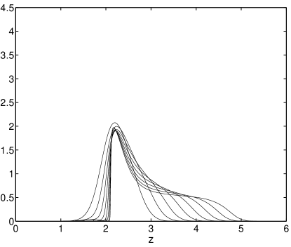
Figure 1: Electron density $n_{e}$ profiles without photoionization. The electrons move to the right following the polarity of the electric field. A negative planar front is developed.

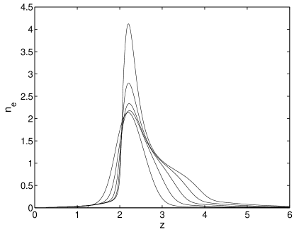
Figure 2: Electron density $n_{e}$ profiles with photoionization, at normal pressure $p=750\,\mbox{Torr}$ and $\gamma=0.21$. A negative front is moving towards the anode at the right and electrons start getting accumulated at the zero electric field plasma zone.

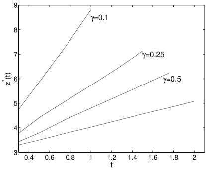
Figure 3: The evolution of a point $z^{*}$ of the negative front at which the electron density has the value $n_{e}=0.1$. When photoionization range $1/\gamma$ is increased, the front moves faster. The line without label belongs to the case where photoionization is neglected.

We can track the motion of the negative front by looking at the time evolution of the point $z^{*}(t)$ at which the electron density has a given value. In Fig.3, we compare the graphs of $z^{*}(t)$ with and without photoionization for a level of $n_{e}=0.1$. As we can see, the effect of photoionization is an acceleration of the negative front which reaches a higher though still constant velocity. This fact holds, after our observations, when one considers kernels $k(s)$ which decay exponentially fast at infinity.

Finally, it is interesting to observe the behaviour of the density $n_{e}$ in the direction opposed to the propagation of the negative front (the left part of the initial distribution). This will be called from now on “the positive front”. We can observe in Fig.2 an effect consisting in the accumulation of electrons in a small region of space in the positive front. This fact is easy to understand by considering the production of electrons away from the positive front which are drifted towards the positive front following the electric field. In the positive front, electrons and positive ions are balanced and hence the net electric field cancels. Therefore electrons cannot proceed any further beyond the positive front and they accumulate there. This is an effect purely associated to photoionization which cannot be explained by invoking any different effect. Unless there is some mechanism allowing the electrons to spread out once they accumulate at the positive front, their density will grow indefinitely and eventually will blow up. We will see in next section that this mechanism is diffusion and the net effect of photoionization and diffusion is the appearance of travelling waves moving towards the cathode, i.e. positive ionization fronts.

VI Photoionization with diffusion: positive ionization fronts

In this section we study in one space dimension the combined effect of photoionization and diffusion on the propagation of positive fronts. The system of equations we study is therefore

$$\frac{\partial n_{e}}{\partial t} = -\frac{\partial}{\partial z}\left(n_{e}E-D\frac{\partial n_{e}}{\partial z}\right)+n_{e}Ee^{-1/E}+S,$$ (64)

$$\frac{\partial n_{p}}{\partial t} = n_{e}Ee^{-1/E}+S,$$ (65)

$$n_{p}-n_{e} = -\frac{\partial E}{\partial z},$$ (66)

where $S$ is the photoionization source term and is written as in equation (57).

The main difference in our approach to this problem with respect to the problem without diffusion is that now an integration along characteristics does not lead to simplifications due to the presence of the second derivatives associated with diffusion. Instead we will use the method of finite differences.

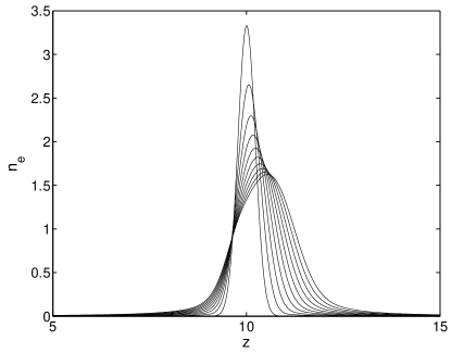
Figure 4: Electron density $n_{e}$ profiles, at normal pressure $p=750\,\mbox{Torr}$, photoionization parameter $\gamma=0.25$ and diffusion $D=0.57$ in dimensionless units. A negative front is moving towards the anode at the right and a positive fronts towards the cathode at the left.

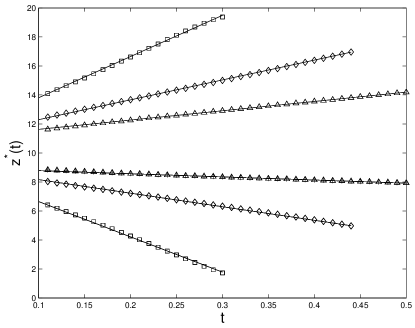
Figure 5: The evolution of points $z^{*}$ of the negative and positive fronts at which the electron density has the value $n_{e}=0.02$. The increasing values are for the negative front and the decreasing ones are for the positive. When photoionization range $1/\gamma$ is increased, the fronts move faster. Triangles $\triangle$ are for $\gamma=0.9$, diamonds $\Diamond$ for $\gamma=0.25$ and squares $\Box$ for $\gamma=0.1$.

In Fig.4, we represent the profiles for $n_{e}$ with $D=0.57$, $p=750\,\mbox{Torr}$ and $\gamma=0.25$. We have used an initial charge distribution which has a maximum at $z=10$. When it evolves, it can be observed a negative planar front developing. The propagation of the negative front is almost identical with or without diffusion when photoionization is present. However there is now a positive front moving towards the cathode. The positive front moves with a constant velocity which is smaller than the velocity of the negative front. In Fig.5 we have plotted the position $z^{*}$ of a point of the negative front and of the positive front which has the particular value of the electron density $n_{e}=0.02$. The parameters are the same as in Fig.4, but for three different values of $\gamma$. For the parameter values chosen above, we have computed the ratio between the velocities of positive and negative fronts: $c_{pos}/c_{neg}=0.34$ for $\gamma=0.9$, $c_{pos}/c_{neg}=0.68$ for $\gamma=0.25$ and $c_{pos}/c_{neg}=0.86$ for $\gamma=0.1$. The ratio grows when the photoionization range $1/\gamma$ increases and the velocities for negative and positive fronts tend to increase and get closer to each other.

The propagation of positive fronts as travelling waves results from the combined action of photoionization and diffusion. This is in contrast with the propagation mechanism for negative fronts, which are also travelling waves but they result from a combination of impact ionization and convection by the electric field. In the latter case, diffusion and photoionization only affect the negative fronts by changing their velocity and their shape. All this conclusions are rather insensitive to the detailed form of the kernel $k(s)$ (see formula (41)) provided it decays exponentially fast at infinity, and hence our conclusions hold with a high degree of generality.

VII Conclusions

In this paper we have studied the effect of photoionization in streamer discharges. We have deduced a minimal model including photoionization and studied with this model the propagation of both positive and negative fronts in the planar case. We have found the appearance of travelling waves which accelerate when the photoionization range increases. For negative fronts we have studied the effect of photoionization both when electronic diffusion is neglected and included. For positive fronts, electronic diffusion has to be taken into account and we have shown how photoionization plays the crucial role pointed by Raether on increasing the velocity of propagation. The control parameter is the photoionization range, i.e. the typical distance at which photons are able to ionize the media. Physically in air, this parameter depends on the amount of oxygen and nitrogen present. It is interesting to point out that for real discharges in the atmosphere, this parameter varies with the altitude.

References

- (1) H. Raether, Die Entwicklung der Elektronenlawine in den Funkenkanal, Z. Phys. 112, 464–489 (1939).
- (2) L. B. Loeb, The problem of the mechanism of static spark discharge, Rev. Mod. Phys. 8, 267–293 (1936).
- (3) M. Arrayás and J. L. Trueba, Investigations of Pre-Breakdown Phenomena: Streamer Discharges, Cont. Phys. 46, 265–276 (2005).
- (4) Y. P. Raizer, Gas Discharge Physics (Springer, Berlin 1991).
- (5) L. B. Loeb and J. M. Meek, The mechanism of the electric spark, Clarendon Press, Oxford, 1941.
- (6) V. P. Pasko, M. A. Stanley, J. D. Mathews, U. S. Inan, and T. G. Wood, Electrical discharge from a thundercloud top to the lower ionosphere, Nature 416, 152–154 (2002).
- (7) M. Arrayás, U. Ebert, and W. Hundsdorfer, Spontaneous branching of anode-directed streamers between planar electrodes, Phys. Rev. Lett. 88, 174502 (2002).
- (8) M. Arrayás, M. A. Fontelos, J. L. Trueba, Mechanism of branching in negative ionization fronts, Phys. Rev. Lett. 95, 165001 (2005).
- (9) S. K. Dhali and A. P. Pal, Numerical simulation of streamers in SF6, J. Appl. Phys. 63, 1355–1362 (1988).
- (10) N. Liu and V. P. Pasko, Effects of photoionization on propagation and branching of positive and negative streamers in sprites, J. Geophys. Res. 109, A04301 (2004).
- (11) G. V. Naidis, On photoionization produced by discharges on air, Plasma Surces Sci. Technol. 15, 253–255 (2006).
- (12) M. B. Zhelezniak, A. Kh. Mnatsakanian, S. V. Sizykh, Photoionization of nitrogen and oxygen mixtures by radiation from a gas discharge, High Temperature, 20, 357–362 (1982).
- (13) P. A. Vitello, B. M. Penetrante, and J. N. Bardsley, Simulation of negative-streamer dynamics in nitrogen, Phys. Rev. E 49, 5574–5598 (1994).
- (14) U. Ebert, W. van Saarloos, and C. Caroli, Streamer propagation as a pattern formation problem: Planar fronts, Phys. Rev. Lett. 77, 4178–4181 (1996), and ibid., Propagation and structure of planar streamer fronts, Phys. Rev. E 55, 1530–1549 (1997).
- (15) M. Arrayás, On negative streamers: A deterministic approach, Am. J. Phys. 72(10), 1283–1289 (2004).
- (16) M. Arrayás, M. A. Fontelos, J. L. Trueba, Ionization fronts in negative corona discharges, Phys. Rev. E 71, 037401 (2005).
- (17) M. Arrayás, M. A. Fontelos, J. L. Trueba, Power laws and self-similar behaviour in negative ionization fronts, J. Phys. A: Math. Gen. 39, 1–18 (2006).
- (18) A. A. Kulikovsky, The role of photoionization in positive streamer dynamics, J. Phys. D: Appl. Phys. 30, 1514–1524 (2000).