Fourier Optics treatment of Classical Relativistic Electrodynamics

Abstract

In this paper we couple Synchrotron Radiation (SR) theory with a branch of physical optics, namely laser beam optics. We show that the theory of laser beams is successful in characterizing radiation fields associated with any SR source. Both radiation beam generated by an ultra-relativistic electron in a magnetic device and laser beam are solutions of the wave equation based on paraxial approximation. It follows that they are similar in all aspects. In the space-frequency domain SR beams appear as laser beams whose transverse extents are large compared with the wavelength. In practical situations (e.g. undulator, bending magnet sources), radiation beams exhibit a virtual ”waist” where the wavefront is often plane. Remarkably, the field distribution of a SR beam across the waist turns out to be strictly related with the inverse Fourier transform of the far-field angle distribution. Then, we take advantage of standard Fourier Optics techniques and apply the Fresnel propagation formula to characterize the SR beam. Altogether, we show that it is possible to reconstruct the near-field distribution of the SR beam outside the magnetic setup from the knowledge of the far-field pattern. The general theory of SR in the near-zone developed in this paper is illustrated for the special cases of undulator radiation, edge radiation and transition undulator radiation. Using known analytical formulas for the far-field pattern and its inverse Fourier transform we find analytical expressions for near-field distributions in terms of far-field distributions. Finally, we compare these expressions with incorrect or incomplete literature.

DEUTSCHES ELEKTRONEN-SYNCHROTRON

in der HELMHOLTZ-GEMEINSCHAFT

DESY 06-127

August 2006

Fourier Optics treatment of Classical Relativistic Electrodynamics

Gianluca Geloni, Evgeni Saldin, Evgeni Schneidmiller and Mikhail Yurkov

Deutsches Elektronen-Synchrotron DESY, Hamburg ISSN 0418-9833 NOTKESTRASSE 85 - 22607 HAMBURG

1 Introduction

In a series of previous works OUR1 , OUR2 , OUR3 we developed a formalism which, we believe, is ideally suited for analysis of any Synchrotron Radiation problem. In particular, in OUR3 we took advantage of Fourier Optics ideas. Fourier Optics (see e.g. GOOD ) provides an extremely successful approach which revolutionized the treatment of wave optics problems and, in particular, laser beam optics problems. It deals with paraxial fields, propagating along a chosen direction (say the longitudinal $z$-axis) and directions close to it. In any given plane transverse to the $z$-axis, the field is represented in the space-frequency domain by a complex scalar function. Alternatively, one may deal with a monochromatic signal oscillating as $\exp[-i\omega t]$, $\omega$ being the frequency and $t$ being the time. Then, one can represent the slowly varying field envelope with a complex scalar function $\widetilde{E}(\vec{r}_{\bot},z)$. Here $z$ is the longitudinal position of the observer, and $\vec{r}_{\bot}$ is a two-dimensional vector identifying transverse coordinates $(x,y)$ of the observer. $\widetilde{E}(\vec{r}_{\bot},z)$ represents an electric field amplitude polarized everywhere in the same, fixed direction. The effects of free-space propagation are mathematically represented by the Fresnel formula. Elementary systems, such as lenses and filters placed along the $z$ axis are introduced as complex scalar-amplitude transmission functions $T(\vec{r}_{\bot})$, which yield the output field after multiplication with an input field. More complex systems are realized by stacking free-space sections and amplitude transmission functions in series.

The use of Fourier Optics led us in a natural way to establish, in this work, basic foundations for the treatment of SR fields in terms of laser beam optics. In particular, radiation from an ultra-relativistic particle can be interpreted as radiation from a virtual source, which produces a laser-like beam. The virtual source itself is the waist of the laser-like beam, and often exhibits a plane wavefront. In this case it is completely specified, for any given polarization component, by a real-valued amplitude distribution of the field. As we will see, the laser-like representation of SR is intimately connected with the ultra-relativistic nature of the electron beam. In particular, paraxial approximation always applies. Then, free space basically acts as a spatial Fourier transformation. This means that the field in the far zone is, aside for a phase factor, the Fourier transform of the field at any position $z$ down the beamline. It is also, aside for a phase factor, the Fourier transform of the virtual source. Once the field at the virtual source is known, the field at other longitudinal positions, both in the far and in the near zone up to distances to the sources comparable with the radiation wavelength, can be obtained with the help of the Fresnel propagation formula. This is equivalent to state that the near-zone field can be calculated from the knowledge of the far-zone field, i.e. from the acceleration term of the Lienard-Wiechert field only. This is possible due to the paraxial approximation. On the one hand, as said above, the Fresnel formula can be used to recover the field up to longitudinal positions which are a wavelength far away from the sources. On the other hand, due to the paraxial approximation, the wavelength of interest in SR emission is very short compared with the radiation formation length and with the linear dimensions of the magnetic setup. In this view, it is incorrect to consider the far-zone field as an asymptotic expression only: its knowledge completely specifies, through the Fresnel integral, the near-zone field as well. In the case when the electron generating the field is not ultra-relativistic, though, the paraxial approximation cannot be applied. As a result, the radiation wavelength is comparable with the radiation formation length. It is then impossible to reconstruct the near-field distribution from the knowledge of the far-field pattern.

In this work we consider a SR source composed of an arbitrary number of magnetic devices under the standard ultra-relativistic approximation. We show that every such magnetic setup is equivalent to several virtual sources and can be modelled as a sequence of appropriately chosen plane sources inserted between the edges of each magnetic structure. This equivalence provides conceptual insight regarding SR sources and should facilitate their design and analysis. In fact, great simplifications in the solution for the problem of propagation of radiation through a beamline result after adopting our viewpoint. Since the analysis of SR sources can be reduced to that of laser-like sources, it follows that any result, method of analysis or design and any algorithm specifically developed for laser beam optics (e.g. the code ZEMAX ZEMA ) are also applicable to SR sources.

To give an example of the applicability of our method we first consider the case of undulator radiation. We work within the applicability region of the resonance approximation. This means that we consider an undulator with a large number $N_{w}$ of periods, i.e. $N_{w}\gg 1$, and that we are interested in frequencies near the fundamental. We find the field distribution of the virtual source with the help of the far-zone field distribution and we propagate to any distance of interest.

Subsequently, we treat the relatively simple case of edge radiation, studying the emission from a setup composed by a straight section and two bending magnets, upstream and downstream of the straight section. Bright, long-wavelength edge radiation is expected to be emitted by such setup for $\lambda\gg\lambda_{c}$, $\lambda_{c}$ being the critical wavelength of SR produced by bending magnets. In particular, we derived an expression for the field from a straight section that is valid at arbitrary observation position. This result is fundamental importance because, due to the superposition principle, our expression may be used as building block for more complicated setups. We begin calculating an analytical expression for the edge radiation (see, among others, BOSF , CHUN , BOS4 , BOS7 , PROY , BOS2 , BOS3 , WILL ) from a single electron in the far zone. Then, through the virtual-source technique we find novel results in the near zone. Two alternative description of the field propagation are given, based on a single virtual source located in the middle of the edge-radiation setup and based on two virtual sources located at the edges of the setup.

With the help of the knowledge of the edge-radiation case, we turn to analyze a more complicated setup consisting of an undulator preceded and followed by two straight sections and two (upstream and downstream) bending magnets. We restrict ourselves to the long-wavelength region. Edge radiation from this kind of setup is commonly known as Transition Undulator Radiation (TUR). The first study on TUR appeared more than a decade ago KIM1 . In that work it was pointed out for the first time that, since an electron entering or leaving an undulator experiences a sudden change in longitudinal velocity, radiation with broadband spectral features, similar to transition radiation, had to be expected in the low-frequency region in addition to the usual undulator radiation. That paper constituted a theoretical basis for many other studies, developed in the years that followed. We remind here a few BOS4 , KINC , CAST , BOS6 , ROY2 , dealing both with theoretical and experimental issues. More recently, TUR has been given consideration in the framework of large X-Ray Free Electron Laser (XFEL) projects. For example, a characterization of Coherent Transition Radiation from the LCLS undulator has been given in REI1 . A method to obtain intense infrared/visible light pulses naturally synchronized to x-ray pulses from the LCLS XFEL by means of Coherent TUR has been proposed in ADA1 , that should be used for pump-probe experiments in the femtosecond scale resolution. In view of these applications, there is a need to extend the knowledge of TUR to the near zone and to the coherent case.

Specification of what precedes and follows the undulator is of fundamental importance. As has been recognized in particular for TUR many years ago BOS4 , it does make sense to discuss about the intensity distribution of TUR only when a detailed knowledge is given, of what precedes and follows the undulator in a specific setup. According to our novel approach, the two straight sections and the undulator will be associated to virtual sources with plane wavefronts. The field from the setup can then be described, in the near as well as in the far field, as a superposition of laser-like beams, radiating at the same wavelength and separated by different phase shifts.

Our work is organized as follows. In Section 2 we discuss our method in full generality. In fact, the analogy with laser beams can be extended to include SR from setups not discussed in this paper. In the following Section 3 we discuss our method in more detail and we focus on particular issues like the importance of the paraxial approximation, the accuracy of our calculations and a easily misleading relationship between velocity and radiation field. In Section 4 we apply our algorithm to the case of usual undulator radiation. Section 5 is dedicated to the study of the simplest edge radiation setup, composed of a straight section and two bending magnets. An undulator is then added to the setup in Section 6, where radiation is given as a superposition of laser-like beam from different virtual sources. Our findings are compared with results in literature in Section 7. Finally, in Section 8, we come to conclusions.

2 Method for obtaining the electromagnetic field generated by an ultra-relativistic electron

In the present Section 2 we discuss our method in all generality. In the next paragraphs 2.1 and 2.2 we show that radiation from an ultra-relativistic particle can be represented as a laser-like beam with a given virtual source. Our algorithm is based on two separately well-known expressions, the Fresnel propagation formula and a far-field presentation of the electromagnetic field.

2.1 Inverse problem with far-field data

We represent the electric field in time domain $\vec{E}(\vec{r},t)$ as a time-dependent function of an observation point located at position $\vec{r}=\vec{r}_{\bot}+z\vec{z}=x\vec{x}+y\vec{y}+z\vec{z}$, where $\vec{x}$, $\vec{y}$ and $\vec{z}$ are defined as (adimensional) unit vectors along horizontal, vertical and longitudinal direction. The field $\vec{E}(\vec{r},t)$ satisfies, in free space, the source-free wave equation:

$$\left[\nabla^{2}-\frac{1}{c^{2}}\frac{\partial^{2}}{\partial t^{2}}\right]\vec{E}=0~{}.$$ (3)

Here $c$ indicates the speed of light in vacuum. For monochromatic waves of angular frequency $\omega$, the wave amplitude has the form

$$\vec{E}_{\bot}(z,\vec{r}_{\bot},t)=\vec{\bar{E}}_{\bot}(z,\vec{r}_{\bot})\exp\left[-i\omega t\right]+C.C.~{},$$ (4)

where ”C.C.” indicates the complex conjugate of the preceding term and $\vec{\bar{E}}_{\bot}$ describes the variation of the wave amplitude. The vector $\vec{\bar{E}}_{\bot}$ actually represents the amplitude of the electric field in the space-frequency domain.

We assume that the ultra-relativistic approximation is satisfied, that is always the case for SR setups. In this case paraxial approximation applies OUR1 . Paraxial approximation implies a slowly varying envelope of the field with respect to the wavelength. It is therefore convenient to introduce the slowly varying envelope of the transverse field components as

$$\vec{\widetilde{E}}_{\bot}=\vec{\bar{E}}_{\bot}\exp{\left[-i\omega z/c\right]}~{},$$ (5)

where the propagation constant $\omega/c$ is related to the wavelength $\lambda$ by $\omega/c=2\pi/\lambda$. In paraxial approximation and in free space, the following parabolic equation holds for the complex envelope ${\widetilde{E}}$ of the Fourier transform of the electric field along a fixed polarization component:

$$\left({{\nabla}_{\bot}}^{2}+\frac{2i\omega}{c}\frac{\partial}{{\partial{z}}}\right){\widetilde{E}}_{\bot}=0~{}.$$ (6)

The derivatives in the Laplacian operator ${{\nabla}_{\bot}}^{2}$ are taken with respect to the transverse coordinates. One has to solve Eq. (6) with a given initial condition at ${z}$, which defines a Cauchy problem. Note that Eq. (6) is similar to the time-dependent Schroedinger equation. We obtain

$${\widetilde{E}_{\bot}}({z}_{o},\vec{r}_{o\bot})=\frac{i\omega}{2\pi c({z}_{o}-{z})}\int d\vec{{r}^{\prime}}_{\bot}~{}\widetilde{E}_{\bot}(z,\vec{r^{\prime}}_{\bot})\exp{\left[\frac{i\omega\left|{\vec{{r}}}_{o\bot}-\vec{{r}^{\prime}_{\bot}}\right|^{2}}{2c({z}_{o}-{z})}\right]}~{},$$ (7)

where the integral is performed over the transverse plane. It is important to note that since $\tilde{E}$ is a slowly-varying function with respect to the wavelength, within the accuracy of the paraxial approximation one cannot resolve the evolution of the field on a longitudinal scale of order of the wavelength. In order to do so, the paraxial equation Eq. (6) should be replaced by a more general Helmholtz equation.

Next to the propagation equation for the field in free space, Eq. (7), we can discuss a propagation equation for the spatial Fourier transform of the field, which can also be derived from Eq. (6) and will be useful later on. We will indicate the spatial Fourier transform of $\widetilde{E}_{\bot}(z,\vec{r^{\prime}}_{\bot})$ with $\mathrm{F}(z,\vec{u})$:

$$\mathrm{F}\left(z,\vec{u}\right)=\int d\vec{r^{\prime}}_{\bot}\widetilde{E}_{\bot}(z,\vec{r^{\prime}}_{\bot})\exp{\left[i\vec{r^{\prime}}_{\bot}\cdot\vec{u}\right]}~{}.$$ (8)

Eq. (6) can be rewritten in terms of $\mathrm{F}$ as

$$\left({{\nabla}_{\bot}}^{2}+\frac{2i\omega}{c}\frac{\partial}{{\partial{z}}}\right)\left\{\int d\vec{u}~{}\mathrm{F}\left(z,\vec{u}\right)\exp{\left[-i\vec{r}_{\bot}\cdot\vec{u}\right]}\right\}=0~{}.$$ (9)

Eq. (9) requires that

$$\left(-\left|\vec{u}\right|^{2}+\frac{2i\omega}{c}\frac{\partial}{{\partial{z}}}\right)\mathrm{F}\left(z,\vec{u}\right)=0~{}.$$ (10)

Solution of Eq. (10) can be presented as

$$\mathrm{F}\left(z,\vec{u}\right)=\mathrm{F}\left(0,\vec{u}\right)\exp{\left[-\frac{ic|\vec{u}|^{2}z}{2\omega}\right]}~{}.$$ (11)

It should be noted that the definition of $\mathrm{F}(0,\vec{u})$ is a matter of initial conditions. In many practical cases, including the totality of the situation treated in this paper, $\mathrm{F}$ (or $\tilde{E}$) may have no direct physical meaning at $z=0$. For instance, in all cases considered in this paper, $z=0$ is within the magnetic setup. However, $\mathrm{F}(0,\vec{u})$ can be considered as the spatial Fourier transform of the field produced by a virtual source. Such a source is defined by the fact that, supposedly placed at $z=0$, it would produce, at any distance from the magnetic system under study, the same field as the real source does. The result in Eq. (11) is very general. On the one hand, the spatial Fourier transform of the electric field exhibits an almost trivial behavior in $z$, since $|\mathrm{F}(z)|^{2}=\mathrm{const}$. On the other hand, the behavior of the electric field itself is not trivial at all. These properties directly follow from the propagation equation for the field and its Fourier transform.

Let us discuss the physical meaning of Eq. (11). The spatial Fourier transform of the field, $\mathrm{F}(z,\vec{u})$, may be interpreted as a superposition of plane waves (the so-called angular spectrum). Once the frequency $\omega$ is fixed, the wave number $k=\omega/c$ is fixed as well, and a given value of the transverse component of the wave vector $\vec{k}_{\bot}=\vec{u}$ corresponds to a given angle of propagation of a plane wave. Different propagation directions correspond to different distances travelled to get to a certain observation point. Therefore, they also correspond to different phase shifts, which depend on the position along the $z$ axis (see, for example, reference GOOD Section 3.7). Free space basically acts as a Fourier transformation. This means that the field in the far zone is, phase factor and proportionality factor aside, the spatial Fourier transform of the field at any position $z$. We now demonstrate this fact. This proof will directly result in an operative method to calculate the field at the virtual source, once the far field is known. We first recall that if we know the field at a given position $(z,\vec{r^{\prime}}_{\bot})$ we may use Eq. (7) to calculate the field at another position $(z_{o},\vec{r}_{o\bot})$ . Let us now consider the limit $z_{o}\longrightarrow\infty$, with finite ratio $\vec{r}_{o\bot}/z_{o}$. In this case, the exponential function in Eq. (7) can be expanded giving

$${\widetilde{E}}_{\bot}({z}_{o},\vec{r}_{o\bot}) = \frac{i\omega}{2\pi c{z}_{o}}\int d\vec{{r}^{\prime}}_{\bot}~{}\widetilde{E}_{\bot}(z,\vec{r^{\prime}}_{\bot})$$ (13)

$$\times\exp{\left[\frac{i\omega}{{2c{z}_{o}}}\left(|\vec{{r}}_{o\bot}|^{2}-2\vec{{r}}_{o\bot}\cdot\vec{{r}^{\prime}}_{\bot}+\frac{z|\vec{{r}}_{o\bot}|^{2}}{{z}_{o}}\right)\right]}~{}.$$

Letting $\vec{\theta}=\vec{r}_{o\bot}/z_{o}$ we have

$${\widetilde{E}}_{\bot}(\vec{\theta}) = \frac{i\omega}{2\pi c{z}_{o}}\exp{\left[\frac{i\omega|\vec{\theta}|^{2}}{2c}(z_{o}+z)\right]}\mathrm{F}\left(z,-\frac{\omega\vec{\theta}}{c}\right)~{}.$$ (15)

With the help of Eq. (11), Eq. (15) may be presented as

$${\widetilde{E}}_{\bot}(\vec{\theta}) = \frac{i\omega}{2\pi c{z}_{o}}\exp{\left[\frac{i\omega|\vec{\theta}|^{2}}{2c}z_{o}\right]}\mathrm{F}\left(0,-\frac{\omega\vec{\theta}}{c}\right)~{}.$$ (16)

Eq. (16) shows what we wanted to demonstrate: free space basically acts as a Fourier transformation. Also, from Eq. (16) one directly obtains

$${\widetilde{E}}_{\bot}(0,\vec{r}_{\bot}) = \frac{i\omega{z}_{o}}{2\pi c}\int d\vec{\theta}\exp{\left[-\frac{i\omega|\vec{\theta}|^{2}}{2c}z_{o}\right]}{\widetilde{E}}_{\bot}(\vec{\theta})\exp\left[\frac{i\omega}{c}\vec{r}_{\bot}\cdot\vec{\theta}\right]~{},$$ (17)

where the transverse vector $\vec{r}_{\bot}$ defines a transverse position on the virtual source plane at $z=0$. Eq. (17) allows to calculate the field at the virtual source once the field in the far zone is known. Identification of the position $z=0$ with the virtual source position is always possible, but not always convenient (although often it is). In general, if the virtual source is at position $z=z_{s}$, one obtains, from Eq. (15) that Eq. (17) should be modified to

$${\widetilde{E}}_{\bot}(z_{s},\vec{r}_{\bot}) = \frac{i\omega{z}_{o}}{2\pi c}\int d\vec{\theta}\exp{\left[-\frac{i\omega|\vec{\theta}|^{2}}{2c}(z_{o}+z_{s})\right]}{\widetilde{E}}_{\bot}(\vec{\theta})\exp\left[\frac{i\omega}{c}\vec{r}_{\bot}\cdot\vec{\theta}\right]~{}.$$ (18)

2.2 Far-field pattern calculations

All is left to do in order to solve the propagation problem in paraxial approximation is to calculate the field in the far zone. We indicate the electron velocity in units of $c$ with $\vec{\beta}(t^{\prime})$, the Lorentz factor (that will be considered fixed throughout this paper) with $\gamma$, the (negative) charge of the electron with $(-e)$ and the electron trajectory as $\vec{r^{\prime}}(t^{\prime})$. Finally, the direction from the retarded position of the electron to the observer is fixed by the unit vector $\vec{n}$,

$$\vec{n}=\frac{\vec{r}_{o}-\vec{r^{\prime}}(t^{\prime})}{|\vec{r}_{o}-\vec{r^{\prime}}(t^{\prime})|}~{}.$$ (19)

Condition $\vec{n}=\mathrm{constant}$ defines the far-field zone. In this zone, a widely-used result presented in textbooks (see JACK ) holds:

$$\vec{\bar{E}}(\vec{r_{o}},\omega) = -{i\omega e\over{cr_{o}}}\exp\left[\frac{i\omega}{c}\vec{n}\cdot\vec{r}_{o}\right]\int_{-\infty}^{\infty}dt^{\prime}~{}{\vec{n}\times(\vec{n}\times{\vec{\beta}})}\exp\left[i\omega\left(t^{\prime}-{1\over{c}}{\vec{n}\cdot\vec{r^{\prime}}}\right)\right].$$ (20)

The transverse components of the envelope of the field in Eq. (LABEL:revwied) can be written as (see OUR1 )

$$\vec{\widetilde{{E}}}_{\bot}(z_{o},\vec{r}_{\bot o},\omega) = -{i\omega e\over{c^{2}}z_{o}}\int_{-\infty}^{\infty}dz^{\prime}{\exp{\left[i\Phi_{T}\right]}}\left[\left({v_{x}(z^{\prime})\over{c}}\right.\right.$$ (23)

$$\left.\left.-{x_{o}-x^{\prime}(z^{\prime})\over{z_{o}}}\right){\vec{x}}+\left({v_{y}(z^{\prime})\over{c}}-{y_{o}-y^{\prime}(z^{\prime})\over{z_{o}}}\right){\vec{y}}\right]~{},$$

where the total phase $\Phi_{T}$ is

$$\Phi_{T}=\omega\left[{s(z^{\prime})\over{v}}-{z^{\prime}\over{c}}\right]+\omega\left(\frac{1}{z_{o}}+\frac{z^{\prime}}{z_{o}^{2}}\right){\left[x_{o}-x^{\prime}(z^{\prime})\right]^{2}+\left[y_{o}-y^{\prime}(z^{\prime})\right]^{2}\over{2c}}~{}.$$ (24)

Eq. (23) can be obtained starting directly with Maxwell’s equations in the space-frequency domain. Textbooks (see for example JACK ) usually follow a not so direct derivation. They start with the solution of Maxwell’s equation in the space-time domain, the well-known Lienard-Wiechert expression, and they subsequently apply a Fourier transformation. Eq. (23) is automatically subject to the paraxial approximation. Here $v_{x}(z^{\prime})$ and $v_{y}(z^{\prime})$ are the horizontal and the vertical components of the transverse velocity of the electron, while $x^{\prime}(z^{\prime})$ and $y^{\prime}(z^{\prime})$ specify the transverse position of the electron as a function of the longitudinal position. Finally, we define the curvilinear abscissa $s(z^{\prime})=vt^{\prime}(z^{\prime})$, $v$ being the modulus of the velocity of the electron.

Eq. (23) can be used to characterize the far field from an electron moving on any trajectory as long as the ultra-relativistic approximation is satisfied. Then, once the far field is known, Eq. (17) (or Eq. (18)) can be used to calculate the field distribution at the virtual source. Finally, Eq. (7) solves the propagation problem at any observation position $z_{o}$. Note that part of the phase in Eq. (24) compensates with the phase in $|\vec{\theta}|^{2}$ in Eq. (17). If Eq. (23) describes a field with a spherical wavefront with center at $z=0$, such compensation is complete. The centrum of the spherical wavefront is a privileged point, and the plane at $z=0$ exhibits a plane wavefront. This explains why the point $z=0$ is often privileged with respect to others.

Let us conclude this Section with a short summary. We considered the electric field represented in the space-frequency domain. Since the system is ultra-relativistic, paraxial approximation applies. We saw that within the applicability region of the paraxial approximation, all information about the field, both in the near and in the far zone, is encoded in the far zone field alone. An explicit expression for the near field can in fact be recovered with the help of the paraxial Green’s function for Maxwell’s equation. Such Green’s function is the same Green’s function considered in Fourier Optics. This consideration allows to describe simple ultra-relativistic systems like, for instance, an electron moving through a bending magnet, an undulator or a straight section in terms of laser-like beams. Each beam has a virtual source, which often exhibits a plane wavefront and is completely specified, for any given polarization component, by a real-valued amplitude distribution for the field. Note that the square modulus of such distribution can be physically associated with an intensity, and can be detected as the image of a properly placed, ideal converging lens. The Fourier transform of such distribution instead is linked to the electric field in the far zone. Then, once the electric field in the far zone is calculated, a virtual source for the laser-like beam can be specified. Once the field at the virtual source is known, the field at any position can be found by applying usual propagation equations based on Fourier Optics.

3 Discussion

In the present Section 3 we discuss the algorithm proposed in Section 2. First we present a thorough derivation of Eq. (23) based on paraxial Green’s function techniques. Then we discuss the region of applicability and the accuracy of this derivation. Finally, we deal with some delicate question related to the nature of the so-called ”velocity field”.

3.1 A derivation of the electric field based on paraxial Green’s function

Eq. (23) is an expression that can be used to characterize the far field from of an electron moving on any trajectory in paraxial approximation. For the sake of completeness we present, here, a derivation of Eq. (23) based on OUR1 .

Accounting for electromagnetic sources, i.e. in a region of space where current and charge densities are present, the following equation for the field in the space-frequency domain holds in all generality:

$$c^{2}\nabla^{2}\vec{\bar{E}}+\omega^{2}\vec{\bar{E}}=4\pi c^{2}\vec{\nabla}\bar{\rho}-4\pi i\omega\vec{\bar{j}}~{},$$ (25)

where $\bar{\rho}(\vec{r},\omega)$ and $\vec{\bar{j}}(\vec{r},\omega)$ are the Fourier transforms of the charge density $\rho(\vec{r},t)$ and of the current density $\vec{j}(\vec{r},t)$. Eq. (25) is the well-known Helmholtz equation, that has elliptic characteristic. With the help of Eq. (5), Eq. (25) can be written as

$$c^{2}\exp\left[{i\omega z/c}\right]\left(\nabla^{2}+{2i\omega\over{c}}{\partial\over{\partial z}}\right)\vec{\widetilde{E}}=4\pi c^{2}\vec{\nabla}\bar{\rho}-4\pi i\omega\vec{\bar{j}}~{}.$$ (26)

A system of electromagnetic sources in the space-time can be conveniently described by $\rho(\vec{r},t)$ and $\vec{j}(\vec{r},t)$. In this paper we will be concerned about a single electron. Using the Dirac delta distribution, we can write, following OUR1

$$\rho(\vec{r},t)=-e\delta(\vec{r}-\vec{r^{\prime}}(t))=-\frac{e}{v_{z}(z)}\delta(\vec{r}_{\bot}-\vec{r^{\prime}}_{\bot}(z))\delta\left(\frac{s(z)}{v}-t\right)$$ (27)

and

$$\vec{j}(\vec{r},t) = -{e}\vec{v}(t)\delta(\vec{r}-\vec{r^{\prime}}(t))=-\frac{e}{v_{z}(z)}\vec{v}(z)\delta(\vec{r}_{\bot}-\vec{r^{\prime}}_{\bot}(z))\delta\left(\frac{s(z)}{v}-t\right),$$ (28)

where $\vec{r^{\prime}}(t)$ and $\vec{v}(t)$ are, respectively, the position and the velocity of the particle at a given time $t$ in a fixed reference frame, and $v_{z}$ is the longitudinal velocity of the electron.

In the space-frequency domain, Eq. (27) and Eq. (LABEL:curr) transform to:

$$\bar{\rho}(\vec{r_{\bot}},z,\omega)=-{e\over{v_{z}(z)}}\delta\left(\vec{r_{\bot}}-\vec{r^{\prime}_{\bot}}(z)\right)\exp\left[{i\omega s(z)/v}\right]$$ (30)

and

$$\vec{\bar{j}}(\vec{r_{\bot}},z,\omega)=-{e\over{v_{z}(z)}}\vec{v}(z)\delta\left(\vec{r_{\bot}}-\vec{r^{\prime}_{\bot}}(z)\right)\exp\left[{i\omega s(z)/v}\right]~{}.$$ (31)

By substitution in Eq. (26) we obtain

$$\left({\nabla}^{2}+{2i\omega\over{c}}{\partial\over{\partial z}}\right)\vec{\widetilde{E}} = {4\pi e\over{v_{z}(z)}}\exp\left\{{i\omega\left({s(z)\over{v}}-{z\over{c}}\right)}\right\}$$ (33)

$$\times\left[{i\omega\over{c^{2}}}\vec{v}(z)\delta\left(\vec{r_{\bot}}-\vec{r^{\prime}_{\bot}}(z)\right)-\vec{\nabla}\delta\left(\vec{r_{\bot}}-\vec{r^{\prime}_{\bot}}(z)\right)\right]~{}.$$

Eq. (33) is still fully general and may be solved in any fixed reference system $(x,y,z)$ of choice with the help of an appropriate Green’s function.

When the longitudinal velocity of the electron, $v_{z}$, is close to the speed of light $c$ (i.e. $\gamma_{z}^{2}\gg 1$), the Fourier components of the source are almost synchronized with the electromagnetic wave travelling at the speed of light. In this case the phase $\omega({s(z)/{v}}-{z/{c}})$ is a slow function of $z$ compared to the wavelength. For example, in the particular case of motion on a straight section, one has $s(z)=z/v_{z}$, so that $\omega({s(z)/{v}}-{z/{c}})=\omega z/(2\gamma_{z}^{2}c)$, and if $\gamma_{z}^{2}\gg 1$ such phase grows slowly in $z$ with respect to the wavelength. For a more generic motion, one has

$$\omega\left({s(z_{2})-s(z_{1})\over{v}}-{z_{2}-z_{1}\over{c}}\right)=\int_{z_{1}}^{z_{2}}d\bar{z}\frac{\omega}{2\gamma_{z}^{2}(\bar{z})c}~{}.$$ (34)

Mathematically, the phase in Eq. (34) enters in the Green’s function solution of Eq. (33) as a factor in the integrand. As we integrate along $z^{\prime}$, the factor $\omega(s(z^{\prime})/v-z^{\prime}/c)$ leads to an oscillatory behavior of the integrand over a certain integration range in $z^{\prime}$. Such range can be identified with the value of $z_{2}-z_{1}$ for which the right hand side of Eq. (34) is of order unity, and it is naturally defined as the radiation formation length $L_{f}$ of the system at frequency $\omega$. It is easy to see by inspection of Eq. (34) that if $v$ is sensibly smaller than $c$ (but still of order $c$), i.e. $v\sim c$ but $1/\gamma_{z}^{2}\sim 1$, then $L_{f}\sim\lambda$. On the contrary, when $v$ is very close to $c$, i.e. $1/\gamma_{z}^{2}\ll 1$, the right hand side of Eq. (34) is of order unity for $L_{f}=z_{2}-z_{1}\gg\lambda$. When the radiation formation length is much longer than the wavelength, $\vec{\widetilde{E}}$ does not vary much along $z$ on the scale of $\lambda$, that is $\mid\partial_{z}\widetilde{E}_{x,y}\mid\ll\omega/c\mid\widetilde{E}_{x,y}\mid$. Therefore, the second order derivative with respect to $z$ in the $\nabla^{2}$ operator on the left hand side of Eq. (33) is negligible with respect to the first order derivative. Eq. (33) can then be simplified to

$$\left({\nabla_{\bot}}^{2}+{2i\omega\over{c}}{\partial\over{\partial z}}\right)\vec{\widetilde{E}}_{\bot} = {4\pi e\over{c}}\exp\left\{{i\omega\left({s(z)\over{v}}-{z\over{c}}\right)}\right\}$$ (36)

$$\times\left[{i\omega\over{c^{2}}}\vec{v}_{\bot}(z)\delta\left(\vec{r}_{\bot}-\vec{r^{\prime}}_{\bot}(z)\right)-\vec{\nabla}_{\bot}\delta\left(\vec{r}_{\bot}-\vec{r^{\prime}}_{\bot}(z)\right)\right],$$

where we consider transverse components of $\vec{\widetilde{E}}$ only and we substituted $v_{z}(z)$ with $c$, having used the fact that $1/\gamma_{z}^{2}\ll 1$. Eq. (LABEL:incipit2) is Maxwell’s equation in paraxial approximation. In this way we transformed Eq. (33), which is an elliptic partial differential equation, into Eq. (LABEL:incipit2), that is of parabolic type. Note that the applicability of the paraxial approximation depends on the ultra-relativistic assumption $\gamma^{2}\gg 1$ but not on the choice of the $z$ axis. In fact, if the longitudinal $z$ direction is chosen in such a way that $\gamma_{z}^{2}\sim 1$, than the formation length is very short $L_{f}\sim\lambda$, and the radiated field is practically zero. As a result, Eq. (LABEL:incipit2) can always be applied, i.e. the paraxial approximation can always be applied, whenever $\gamma^{2}\gg 1$. Formally, this statement is in contradiction with the approximation $1/\gamma_{z}^{2}\ll 1$, explicitly declared to obtain Maxwell’s equation in paraxial approximation, i.e. Eq. (LABEL:incipit2). However, suppose that one is using a detector not accurate enough to distinguish, on an axis where $\gamma_{z}^{2}\gg 1$, between solution of Maxwell’s equation with paraxial approximation and solution without it. Let us fix any observation wavelength of interest $\lambda$. Then, with the accuracy of the paraxial approximation, one would detect no photon flux along an axis where $\gamma_{z}^{2}\sim 1$. Thus, from a practical viewpoint, the paraxial approximation can always be applied independently of $\gamma_{z}$. When it is not formally applicable, the error resulting from its application cannot be resolved by our detector, within the accuracy of the paraxial approximation, because we are working with ultra-relativistic particles, and radiation is highly collimated. In this regard, it should be remarked here that the status of the paraxial equation Eq. (LABEL:incipit2) in Synchrotron Radiation theory is different from that of the paraxial equation in Physical Optics. In the latter case, the paraxial approximation is satisfied only by small observation angles. For example, one may think of a setup where a thermal source is studied by an observer positioned at a long distance from the source and behind a limiting aperture. Only if a small-angle acceptance is considered the paraxial approximation can be applied. On the contrary, due to the ultra-relativistic nature of the electrons that generate radiation, Synchrotron Radiation is highly collimated. As a result the paraxial equation can always be applied in practice, because it practically returns zero field at angles where it should not be applied.

The Green’s function for Eq. (LABEL:incipit2), namely the solution corresponding to the unit point source, satisfies the equation

$$\left({\nabla_{\bot}}^{2}+{2i\omega\over{c}}{\partial\over{\partial z}}\right)G(z_{o}-z;\vec{r_{\bot o}}-\vec{r_{\bot}})=\delta(\vec{r_{\bot o}}-\vec{r_{\bot}})\delta(z_{o}-z)~{},$$ (38)

and, in an unbounded region, can be explicitly written as

$$G(z_{o}-z^{\prime};\vec{r}_{\bot o}-\vec{r^{\prime}}_{\bot})=-{1\over{4\pi(z_{o}-z^{\prime})}}\exp\left\{i\omega{\mid\vec{r}_{\bot o}-\vec{r^{\prime}}_{\bot}\mid^{2}\over{2c(z_{o}-z^{\prime})}}\right\}~{},$$ (39)

assuming $z_{o}-z^{\prime}>0$. When $z_{o}-z^{\prime}<0$ the paraxial approximation does not hold, and the paraxial wave equation Eq. (LABEL:incipit2) should be substituted, in the space-frequency domain, by the more general Helmholtz equation. However, the radiation formation length for $z_{o}-z^{\prime}<0$ is very short with respect to the case $z_{o}-z^{\prime}>0$, i.e. there is no radiation for observer positions $z_{o}-z^{\prime}<0$. As a result, in this paper we will consider only $z_{o}-z^{\prime}>0$. It follows that the observer is located downstream of the sources.

This leads to the solution

$$\vec{\widetilde{E}}_{\bot}(z_{o},\vec{r}_{\bot o},\omega) = -{e\over{c}}\int_{-\infty}^{\infty}dz^{\prime}{1\over{z_{o}-z^{\prime}}}\int d\vec{r^{\prime}}_{\bot}$$ (42)

$$\times\left[{i\omega\over{c^{2}}}\vec{v_{\bot}}(z^{\prime})\delta\left(\vec{r^{\prime}}_{\bot}-\vec{r^{\prime}}_{\bot}(z^{\prime})\right)-\vec{\nabla^{\prime}}_{\bot}\delta\left(\vec{r^{\prime}}_{\bot}-\vec{r^{\prime}}_{\bot}(z^{\prime})\right)\right]$$

$$\times\exp\left\{i\omega\left[{\mid\vec{r}_{\bot o}-\vec{r^{\prime}}_{\bot}\mid^{2}\over{2c(z_{o}-z^{\prime})}}+\left({s(z^{\prime})\over{v}}-{z^{\prime}\over{c}}\right)\right]\right\}~{},$$

where $\vec{\nabla^{\prime}}_{\bot}$ represents the gradient operator with respect to the source point. The integration over transverse coordinates can be carried out leading to the final result:

$$\vec{\widetilde{E}}_{\bot}(z_{o},\vec{r}_{\bot o},\omega) = -{i\omega e\over{c^{2}}}\int_{-\infty}^{\infty}dz^{\prime}\frac{\exp\left[{i\Phi_{T}}\right]}{z_{o}-z^{\prime}}\left[\left({v_{x}(z^{\prime})\over{c}}\right.\right.$$ (44)

$$\left.\left.-{x_{o}-x^{\prime}(z^{\prime})\over{z_{o}-z^{\prime}}}\right)\vec{x}+\left({v_{y}(z^{\prime})\over{c}}-{y_{o}-y^{\prime}(z^{\prime})\over{z_{o}-z^{\prime}}}\right)\vec{y}\right]~{},$$

where the total phase $\Phi_{T}$ is given by

$$\Phi_{T}=\omega\left[{s(z^{\prime})\over{v}}-{z^{\prime}\over{c}}\right]+\omega\left[{\left(x_{o}-x^{\prime}(z^{\prime})\right)^{2}+\left(y_{o}-y^{\prime}(z^{\prime})\right)^{2}\over{2c(z_{o}-z^{\prime})}}\right]~{}.$$ (45)

As we will see in Section 3.2, Eq. (44) is valid at any observation position $z_{o}$ such that the paraxial approximation is valid, i.e. up to distances between the observer and the electromagnetic sources comparable with the radiation wavelength. In the far zone Eq. (44) reduces to Eq. (23).

3.2 Exact solution of Helmholtz equation

Up to now we presented an algorithm based on the paraxial approximation. It makes sense to ask what is the range of observer positions where the paraxial approximation applies, and what is the accuracy of our result in this range. We will demonstrate that paraxial approximation holds with good accuracy up to positions of the observer such that its distance from the electromagnetic sources in the space-frequency domain, denoted with $d$, is of order of $\lambda$.

In order to investigate the accuracy of our findings we have to compare results from the paraxial treatment with results obtained within a more general framework without the help of the paraxial approximation. Therefore we go back to the most general Eq. (25), that can be solved by direct application of the Green’s function for the Helmholtz equation

$$G(\vec{r}_{o}-\vec{r^{\prime}}) = -{1\over{4\pi\left|\vec{r}_{o}-\vec{r^{\prime}}\right|}}\exp\left\{i{\omega\over{c}}{\mid\vec{r}_{o}-\vec{r^{\prime}}\mid}\right\}~{},$$ (46)

that automatically includes the Sommerfeld radiation condition

$$|\vec{r_{o}}-\vec{r^{\prime}}|\left(\frac{\partial G}{\partial\vec{n}}-i\frac{cG}{\omega}\right)\longrightarrow 0~{}~{}~{}~{}\mathrm{as}~{}~{}|\vec{r_{o}}-\vec{r^{\prime}}|\longrightarrow\infty~{}.$$ (47)

Integrating by parts the term in $\vec{\nabla}\bar{\rho}$ we have

$$\vec{\bar{E}} = -\int d\vec{r^{\prime}}\left[{i\omega\over{c\left|\vec{r_{o}}-\vec{r^{\prime}}\right|}}\left(\bar{\rho}\vec{n}-{\vec{\bar{j}}\over{c}}\right)+{\bar{\rho}\vec{n}\over{\left|\vec{r_{o}}-\vec{r^{\prime}}\right|^{2}}}\right]\exp\left\{i{\omega\over{c}}{\mid\vec{r_{o}}-\vec{r^{\prime}}\mid}\right\}~{}.$$ (48)

Use of explicit expressions for $\bar{\rho}$, i.e. Eq. (30), and for $\vec{\bar{j}}$, i.e. Eq. (31), leads straightforwardly to the following expression for the field envelope:

$$\vec{\widetilde{E}}(\vec{r_{o}},\omega) = -{i\omega e\over{c}}\int_{-\infty}^{\infty}dz^{\prime}{1\over{v_{z}(z^{\prime})}}\left[{\vec{\beta}-\vec{n}\over{|\vec{r_{o}}-\vec{r^{\prime}}(z^{\prime})|}}-{ic\over{\omega}}{\vec{n}\over{|\vec{r_{o}}-\vec{r^{\prime}}(z^{\prime})|^{2}}}\right]$$ (50)

$$\times\exp\left\{i\omega\left[\left({s(z^{\prime})\over{v}}-{z^{\prime}\over{c}}\right)+\left({|\vec{r_{o}}-\vec{r^{\prime}}(z^{\prime})|\over{c}}-{z_{o}-z^{\prime}\over{c}}\right)\right]\right\}~{}.$$

It should be emphasized that in usual Physical Optics cases one is interested in solving Maxwell’s equations with particular boundary conditions. Typically, boundary conditions are artificial and not consistent with Maxwell’s equation. Thus, it is not possible to control approximations applied. On the contrary, in our case, Eq. (50) is an exact solution of Maxwell’s equations with boundary conditions at infinity. In this case the scalar Green’s function in Eq. (46) can be used without introducing any extra assumption. These situations are completely different. The exactness of the solution in Eq. (50) allows us to control the overall accuracy of the paraxial approximation by comparing results from Eq. (44) with results from the exact solution of Maxwell’s equations, Eq. (50). We can present here a conservative estimate. Let us pose

$$\lambdabar=\frac{\lambda}{2\pi}~{}.$$ (51)

When $d\gtrsim L_{f}$ this accuracy can be estimated to amount to $\lambdabar/L_{f}$, but quickly decreases as $L_{f}\gg d\gg\lambdabar$ remaining, at least, of order of $\lambdabar/d$. The words ”at least” emphasize the before-mentioned fact that this is a conservative estimate.

The most general conclusion that can be drawn from Eq. (50) is that, independently of any approximation, the use of the space-frequency domain automatically presents a very natural scale, the wavelength $\lambda$. As it can be verified by inspecting Eq. (50), the integrand term scaling as $|\vec{r_{o}}-\vec{r^{\prime}}(z^{\prime})|^{-2}$ can be dropped whenever $d\gg\lambda$. This is to be taken as a sufficient condition, but not necessary in general. Dropping this term is automatically enforced when the paraxial approximation is applied, but it is not sufficient for the paraxial approximation to hold. In order for the paraxial approximation to hold, as seen before, the system must be ultra-relativistic.

While the present discussion about Helmholtz equation is important to understand the region of applicability of Eq. (44) we should stress the fact that the inverse field problem, which relies on far-field data only, cannot be solved without application of the paraxial approximation. In fact, let us suppose that the paraxial approximation was not applicable. Then, instead of Eq. (6) we should solve the homogeneous Helmholtz equation

$$c^{2}\nabla^{2}\vec{\bar{E}}+\omega^{2}\vec{\bar{E}}=0~{}.$$ (52)

Boundary conditions are now constituted by the knowledge of the field on a open surface (for example, a transverse plane) and additionally, Rayleigh-Sommerfeld radiation condition (separately for all polarization components) at infinity, i.e.

$$|\vec{r_{o}}-\vec{r^{\prime}}|\left(\frac{\partial\bar{E}_{x,y}}{\partial\vec{n}}-i\frac{c\bar{E}_{x,y}}{\omega}\right)\longrightarrow 0~{}~{}~{}~{}\mathrm{as}~{}~{}|\vec{r_{o}}-\vec{r^{\prime}}|\longrightarrow\infty~{}.$$ (53)

However, this is not enough to reconstruct the field at any position in space. In order to do so, we would need to specify the sources. In this case though, Eq. (48) can be directly applied. The boundary conditions specified above allow one to solve the direct transmission problem, but not the inverse one. However, as we have seen, if the paraxial approximation is applicable, the inverse field problem has unique and stable solution.

Based on this discussion we can formulate a definition of several observation zones of interest (together with their complementary zones in square brackets).

• Far zone [Near zone]. Defined by $d$ such that $\vec{n}=\mathrm{const.}$ [for the near zone read: $\vec{n}\neq\mathrm{const.}$] throughout the integration in Eq. (50).

• Formation zone [Non-formation zone]. Defined by $d\lesssim L_{f}$ [for the non-formation zone read: $d\gg L_{f}$] .

• Radiation zone [Non-radiation zone] . Defined by $d$ such that the electromagnetic field is disentangled [for the non-radiation zone read: entangled] from the particle field and can be interpreted as radiation.

• $\mathbf{1/R-}$zone [$\mathbf{1/R^{2}-}$zone] . Defined by $d$ such that the term in $1/R^{2}=|\vec{r_{o}}-\vec{r^{\prime}}(z^{\prime})|^{-2}$ can be neglected [for the ${1/R^{2}-}$zone read: cannot be neglected] in the integrand of Eq. (50).

• Reconstruction zone [Non-reconstruction zone]. Defined by $d$ such that a solution of the inverse problem based on far-field data can be given [for the non-reconstruction zone read: cannot be given].

In all generality, from Eq. (50) follows that the $1/R-$zone always coincides with the reconstruction zone, because field can be reconstructed from the far-zone data if and only if the term containing $1/R^{2}$ in the integrand of Eq. (50) can be neglected. This is clear because the far-zone data do not include the term in Eq. (50). Moreover if an observer is in the $1/R-$zone (or in the reconstruction zone), it necessarily belongs to the radiation zone as well. However we cannot prove, in general, that if an observer is in the radiation zone, it necessarily belongs to the $1/R-$zone (or to the reconstruction zone).

Let us now consider a slightly less general standpoint and discuss, independently of the paraxial approximation, both non-ultra-relativistic systems, such that $\beta\simeq 1$ and $\gamma^{2}\simeq 1$, and ultra-relativistic systems such that $\gamma^{2}\gg 1$ (and obviously $\beta\simeq 1$).

In the case of non-ultra-relativistic systems the characteristic size of the system $a$, the formation length $L_{f}$ and the radiation wavelength $\lambda$ are of the same magnitude. As a result, there are only two observation zones of interest. The first, such that $d\gg\lambdabar$, incorporates far zone, non-formation zone, radiation zone, $1/R-$zone and reconstruction zone. The second, such that $d\lesssim\lambdabar$, incorporates near zone, formation zone, non-radiation zone, $1/R^{2}-$zone and non-reconstruction zone.

In the case of ultra-relativistic systems instead, we can say that $a\gtrsim L_{f}$ and $L_{f}\gg\lambda$. As a result the near zone is now defined by $d\lesssim a$, the formation zone by $d\lesssim L_{f}$, the radiation zone by $d\gg\lambdabar$. As for the reconstruction zone and the $1/R-$zone we can say that a necessary and sufficient condition to be in these zones is that $d\gg\lambdabar$.

3.3 Radiation contribution from the ”velocity field”

As one can see, the case of ultra-relativistic system presents an increased level of complexity with respect to the non-ultra-relativistic system. This complexity is at the origin of several misconceptions, that we here discuss.

We presented, in the space-frequency domain, an exact solution of Maxwell’s equation, Eq. (50) (and its paraxial form Eq.(44)), starting directly with Maxwell’s equations in the space-frequency domain. As said before, textbooks (see for example JACK ) usually follow a not so direct derivation. They start with the solution of Maxwell’s equation in the space-time domain, the well-known Lienard-Wiechert expression, and they subsequently apply a Fourier transformation. The Lienard-Wiechert expression for the electric field of a point charge $(-e)$ reads (see, e.g. JACK ):

$$\vec{{E}}(\vec{r}_{o},t) = -e{\vec{n}-\vec{\beta}\over{\gamma^{2}(1-\vec{n}\cdot\vec{\beta})^{2}|\vec{r}_{o}-\vec{r^{\prime}}|^{2}}}-{e\over{c}}{\vec{n}\times[(\vec{n}-\vec{\beta})\times\dot{\vec{\beta}}]\over{(1-\vec{n}\cdot\vec{\beta})^{2}|\vec{r}_{o}-\vec{r^{\prime}}|}}.$$ (54)

As before, $R=|\vec{r}_{o}-\vec{r^{\prime}}(t^{\prime})|$ denotes the displacement vector from the retarded position of the charge to the point where the fields are calculated. Moreover, $\vec{\beta}=\vec{v}/c$, $\vec{\dot{\beta}}=\vec{\dot{v}}/c$, while $\vec{v}$ and $\vec{\dot{v}}$ denote the retarded velocity and acceleration of the electron. Finally, the observation time $t$ is linked with the retarded time $t^{\prime}$ by the retardation condition $R=c(t-t^{\prime})$. As is well-known, Eq. (54) serves as a basis for the decomposition of the electric field into a sum of two quantities. The first term on the right-hand side of Eq. (54) is independent of acceleration, while the second term linearly depends on it. For this reason, the first term is called ”velocity field”, and the second ”acceleration field” JACK . Velocity fields differ from acceleration fields in several respects, one of which is the behavior in the limit for a very large distance from the electron. There one finds that the velocity fields decrease like $R^{-2}$, while acceleration fields only decrease as $R^{-1}$. Let us apply a Fourier transformation:

$$\vec{\bar{E}}(\vec{r}_{o},\omega) = -e\int_{-\infty}^{\infty}dt^{\prime}{\vec{n}-\vec{\beta}\over{\gamma^{2}(1-\vec{n}\cdot\vec{\beta})^{2}|\vec{r}_{o}-\vec{r^{\prime}}|^{2}}}\exp\left[i\omega\left(t^{\prime}+{|\vec{r}_{o}-\vec{r^{\prime}}(t^{\prime})|\over{c}}\right)\right]$$ (56)

$$-{e\over{c}}\int_{-\infty}^{\infty}dt^{\prime}{\vec{n}\times[(\vec{n}-\vec{\beta})\times\dot{\vec{\beta}}]\over{(1-\vec{n}\cdot\vec{\beta})^{2}|\vec{r}_{o}-\vec{r^{\prime}}|}}\exp\left[i\omega\left(t^{\prime}+{|\vec{r}_{o}-\vec{r^{\prime}}(t^{\prime})|\over{c}}\right)\right].$$

As in Eq. (54) one may formally recognize a velocity and an acceleration term in Eq. (56) as well. Since Eq. (56) follows directly from Eq. (54), that is valid in the time domain, the magnitude of the velocity and acceleration parts in Eq. (56), that include terms in $1/R^{2}$ and $1/R$ respectively, do not depend on the wavelength $\lambda$. On the contrary, as we have seen, the terms including $1/R$ and $1/R^{2}$ in Eq. (50) do. It is instructive to take advantage of integration by parts to show that Eq. (50) and Eq. (54) are equivalent. With the help of

$${1\over{c}}{d\over{dt^{\prime}}}|\vec{r_{o}}-\vec{r^{\prime}}(t^{\prime})|=-\vec{n}\cdot\vec{\beta}~{}.$$ (57)

and

$${d\vec{n}\over{dt^{\prime}}}={c\over{|\vec{r}_{o}-\vec{r^{\prime}}(t^{\prime})|}}\left[-\vec{\beta}+\vec{n}\left(\vec{n}\cdot\vec{\beta}\right)\right]~{},$$ (58)

Eq. (56) can be written as

$$\vec{\bar{E}} ( \vec{r}_{o},\omega)=-{e}\int_{-\infty}^{\infty}dt^{\prime}{\vec{n}\over{|\vec{r}_{o}-\vec{r^{\prime}}(t^{\prime})|^{2}}}\exp\left[i\omega\left(t^{\prime}+{|\vec{r}_{o}-\vec{r^{\prime}}(t^{\prime})|\over{c}}\right)\right]$$ (60)

$$+{e\over{c}}\int_{-\infty}^{\infty}dt^{\prime}{d\over{dt^{\prime}}}\left[{\vec{\beta}-\vec{n}\over{({1-\vec{n}\cdot\vec{\beta}})|\vec{r}_{o}-\vec{r^{\prime}}(t^{\prime})|}}\right]\exp\left[i\omega\left(t^{\prime}+{|\vec{r}_{o}-\vec{r^{\prime}}(t^{\prime})|\over{c}}\right)\right].$$

Eq. (LABEL:revtrasfbiss) may now be integrated by parts. When edge terms can be dropped one obtains

$$\vec{\bar{E}}(\vec{r_{o}},\omega) = -{i\omega e\over{c}}\int_{-\infty}^{\infty}dt^{\prime}\left[{\vec{\beta}-\vec{n}\over{|\vec{r_{o}}-\vec{r^{\prime}}(t^{\prime})|}}-{ic\over{\omega}}{\vec{n}\over{|\vec{r_{o}}-\vec{r^{\prime}}(t^{\prime})|^{2}}}\right]$$ (63)

$$\times\exp\left\{i\omega\left(t^{\prime}+{|\vec{r_{o}}-\vec{r^{\prime}}(t^{\prime})|\over{c}}\right)\right\}~{}.$$

Recalling $t^{\prime}=z^{\prime}/v_{z}(z^{\prime})=s(z^{\prime})/v$ and the definition in Eq. (5) one sees that Eq. (63) is equivalent to Eq. (50). Eq. (63) is the starting point for numerical codes based on direct calculation of the near field (the most well-known example is perhaps SRW CHU2 ).

The derivation of Eq. (63) is particularly instructive because shows that each term in Eq. (63) is due to a combination of velocity and acceleration terms in Eq. (56). In other words the terms in $1/R$ and in $1/R^{2}$ in Eq. (63) appear as a combination of the terms in $1/R$ (acceleration term) and $1/R^{2}$ (velocity term) in Eq. (56). As a result, one can say that there exist contributions to the radiation from the velocity part in Eq. (56). The presentation in Eq. (63) (or Eq. (50)) is more interesting with respect to that in Eq. (56) (although equivalent to it) because the magnitude of the $1/R^{2}$-term in Eq. (63) can be directly compared with the magnitude of the $1/R$-term inside the sign of integral, and is related, as we have seen, to the $1/R$-zone and to the reconstruction zone, where the field can be reconstructed from far-field data. It must be clear that the $1/R^{2}$-term in Eq. (63) does not coincide with the $1/R^{2}$-term in Eq. (56), that is the velocity field. If one forgets about this fact he would come to the paradoxical conclusion that far-field data can be used to reconstruct the field in the far-zone only (on the contrary, we have seen that when $d\gg\lambdabar$ we are in the reconstruction zone). Note that while this conclusion is, in general, a misconception, it does give incorrect results in the case of ultra-relativistic systems only, because in the case of non-ultra-relativistic systems the reconstruction zone and the far zone coincide.

The bottom line is that only to the integral in Eq. (56) or Eq. (63) can be ascribed physical sense. The integrand is, in fact, an artificial construction. In this regard, it is interesting to note that the integration by parts giving Eq. (63) is not unique. An expression equivalent to Eq. (63) for the Fourier transform of the electric fields can be found in the very interesting, but perhaps little known reference LUCC . After starting with Eq. (56), the authors of LUCC organized integration by part in a different way compared with what has been done in Eq. (LABEL:revtrasfbiss). First they found that

$${\vec{n}\times[(\vec{n}-\vec{\beta})\times\vec{\dot{\beta}}]\over{|\vec{r_{o}}-\vec{r^{\prime}}|(1-\vec{n}\cdot\vec{\beta})^{2}}} = {1\over{|\vec{r_{o}}-\vec{r^{\prime}}|}}{d\over{dt^{\prime}}}\left[{\vec{n}\times(\vec{n}\times\vec{\beta})\over{(1-\vec{n}\cdot\vec{\beta})}}\right]$$ (65)

$$-\left[{\vec{\dot{n}}(\vec{n}\cdot\vec{\beta})+\vec{n}(\vec{\dot{n}}\cdot\vec{\beta})-\vec{\dot{n}}(\vec{n}\cdot\vec{\beta})^{2}-\vec{\beta}(\vec{\dot{n}}\cdot\vec{\beta})\over{|\vec{r_{o}}-\vec{r^{\prime}}|(1-\vec{n}\cdot\vec{\beta})^{2}}}\right].$$

Note that Eq. (65) accounts for the fact that $\vec{n}=(\vec{r_{o}}-\vec{r^{\prime}}(t^{\prime}))/|\vec{r_{o}}-\vec{r^{\prime}}(t^{\prime})|$ is not a constant in time. Using Eq. (65) in the integration by parts, authors of LUCC obtained

$$\vec{\bar{E}}(\vec{r_{o}},\omega) = -{i\omega e\over{c}}\int_{-\infty}^{\infty}dt^{\prime}\left[-{\vec{n}\times(\vec{n}\times{\vec{\beta}})\over{|\vec{r_{o}}-\vec{r^{\prime}}(t^{\prime})|}}+{i{c}\over{\omega}}{\vec{\beta}-\vec{n}-2\vec{n}(\vec{n}\cdot\vec{\beta})\over{|\vec{r_{o}}-\vec{r^{\prime}}(t^{\prime})|^{2}}}\right]$$ (67)

$$\times\exp\left\{i\omega\left(t^{\prime}+{|\vec{r_{o}}-\vec{r^{\prime}}(t^{\prime})|\over{c}}\right)\right\}~{}.$$

Similarly as before, the edge terms have been dropped. Eq. (56), Eq. (63) and Eq. (67) are equivalent but include different integrands. This is no mistake, as different integrands can lead to the same integral.

Another way to state this fact, in a more general way, is that Eq. (56), Eq. (63) and Eq. (67) can be obtained one from the other by means of the addition of a full derivative to the respective integrals. For example, the integration by parts used to transform Eq. (56) into Eq. (63) is equivalent to add to the integrand of Eq. (56) the full derivative $d\Omega_{1}/dt^{\prime}$ of the quantity

$$\Omega_{1}=-{\vec{\beta}-\vec{n}\over{({1-\vec{n}\cdot\vec{\beta}})|\vec{r}_{o}-\vec{r^{\prime}}(t^{\prime})|}}\exp\left[i\omega\left(t^{\prime}+{|\vec{r}_{o}-\vec{r^{\prime}}(t^{\prime})|\over{c}}\right)\right]~{},$$ (68)

while the integration by parts used to transform Eq. (56) into Eq. (67) is equivalent to add to the integrand of Eq. (56) the full derivative $d\Omega_{2}/dt^{\prime}$ of the quantity

$$\Omega_{2}=-{\vec{n}\times(\vec{n}\times\vec{\beta})\over{(1-\vec{n}\cdot\vec{\beta})|\vec{r}_{o}-\vec{r^{\prime}}(t^{\prime})|}}\exp\left[i\omega\left(t^{\prime}+{|\vec{r}_{o}-\vec{r^{\prime}}(t^{\prime})|\over{c}}\right)\right]~{}.$$ (69)

There are infinite full derivatives of functions $\Omega$ that can be summed to the integrand of the field-integral, giving infinite representations of the same physical quantity, the electric field. From this viewpoint, summing a full derivative to the integrand of the field-integral is analogous to a gauge transformation, that leaves invariant the observable quantity (the field), but transforms the electromagnetic potential in ways that may be useful in particular situations. Of all possible choice of $\Omega$, the function $\Omega_{1}$, that gives Eq. (63), is particularly useful because, as we have seen, the magnitude of the $1/R^{2}$-term in Eq. (63) can be directly compared with the magnitude of the $1/R$-term inside the sign of integral. However, the field obtained by summing full derivatives to the integrand is invariant for any choice of $\Omega$.

Let us summarize the result of this discussion. We have seen how different zones scale with the other characteristic lengths of the problem, the wavelength $\lambda$, the formation length $L_{f}$ and the typical dimension of the system $a$. Complexities arise in the ultra-relativistic case, when $\lambda$, $a$ and $L_{f}$ are very different quantities. In particular far zone, reconstruction zone and radiation zone are, in general, different concepts. Due to this fact, paradoxes may arise when ascribing separate meaning to velocity and acceleration part of the Lienard-Wiechert fields after Fourier transformation, i.e. in Eq. (54). In particular, we have shown that the integrand of the field-integral has no physical meaning. However, the representation of the field integral in Eq. (63) is particularly important, as it allows a better physical insight, very much as a particular choice of electromagnetic gauge can do in particular situations.

4 Application 1. Undulator radiation as a laser-like beam

An important exemplification of our algorithm is given here for the particular case of undulator radiation. We assume, for simplicity, that the resonance condition with the fundamental harmonic is satisfied, that is

$$\frac{\omega}{2\gamma^{2}c}\left(1+\frac{K^{2}}{2}\right)=\frac{2\pi}{\lambda_{w}}~{},$$ (70)

where $\lambda_{w}$ is the undulator period, while $K$ is the undulator parameter

$$K=\frac{\lambda_{w}eH_{w}}{2\pi m_{\mathrm{e}}c^{2}}~{},$$ (71)

$m_{\mathrm{e}}$ being the electron mass and $H_{w}$ being the maximum of the magnetic field produced by the undulator on the $z$ axis.

We also specify that position $z=0$ is taken in the middle of the undulator. We consider a planar undulator, so that the transverse velocity of an electron can be written as

$$\vec{v}_{\bot}(z^{\prime})=-{cK\over{\gamma}}\sin{\left(k_{w}z^{\prime}\right)}\vec{x}~{}.$$ (72)

A well-known expression for the angular distribution of the first harmonic field in the far-zone can be obtained from Eq. (23) or Eq. (LABEL:revwied). Such expression is axis-symmetric, and can therefore be presented as a function of a single observation angle $\theta$, where

$$\theta^{2}=\theta_{x}^{2}+\theta_{y}^{2}~{},$$ (73)

$\theta_{x}$ and $\theta_{y}$ being angles measured from the undulator $z$-axis in the horizontal and in the vertical direction. One obtains the following distribution:

$$\widetilde{{E}}_{\bot}(z_{o},\theta) = -\frac{K\omega eL_{w}}{c^{2}z_{o}\gamma}A_{JJ}\exp\left[i\frac{\omega z_{o}}{2c}\theta^{2}\right]\mathrm{sinc}\left[\frac{\omega L_{w}\theta^{2}}{4c}\right]~{},$$ (74)

where the field is polarized in the horizontal direction. Here $L_{w}=\lambda_{w}N_{w}$ is the undulator length and $N_{w}$ the number of undulator periods. Finally, $A_{JJ}$ is defined as

$$A_{JJ}=J_{o}\left(\frac{K^{2}}{4+2K^{2}}\right)-J_{1}\left(\frac{K^{2}}{4+2K^{2}}\right)~{},$$ (75)

$J_{n}$ being the n-th order Bessel function of the first kind. Eq.(74) describes a field with spherical wavefront centered in the middle of the undulator. Eq. (17) can now be used to calculate the field distribution at the virtual source yielding

$$\widetilde{{E}}_{\bot}(0,r_{\bot}) = i\frac{K\omega e}{c^{2}\gamma}A_{JJ}\left[\pi-2\mathrm{Si}\left(\frac{\omega{r}_{\bot}^{2}}{L_{w}c}\right)\right]~{},$$ (76)

where $\mathrm{Si}(\cdot)$ indicates the sin integral function and $r_{\bot}=|\vec{r}_{\bot}|$ is the distance from the $z$ axis on the virtual-source plane. Note that $\widetilde{{E}}_{\bot}(0,r_{\bot})$ is axis-symmetric. Eq. (76), that has been already presented in OUR3 , describes a virtual field with a plane wavefront. Let us compare this virtual field with a laser-beam waist. In laser physics, the waist is located in the center of the optical cavity. In analogy with this, in our case the virtual source is located in the center of the undulator. Both in laser physics and in our situation the waist has a plane phase front and the transverse dimension of the waist is much longer than the wavelength. Note that the phase of the wavefront in Eq. (76) is shifted of $-\pi/2$ with respect to the spherical wavefront in the far zone. Such phase shift is analogous to the Guoy phase shift in laser physics. Finally, in laser physics, the Rayleigh range for a laser beam is presented in the form $z_{R}=(\omega/c)w_{o}^{2}$, $w_{o}$ being the radius of the beam at the location of the waist (i.e. at that position along $z$ where the phase front is flat). This is defined, for example, by requiring that the intensity on the edge of an aperture of radius $w_{o}$ be one fourth of the intensity at the center of the radiation spot. In the undulator source case, the definition given above amounts to $w_{o}=0.9(cL_{w}/\omega)^{1/2}$ and $z_{R}=0.8L_{w}\simeq L_{w}$. In the case of a laser beam the Rayleigh length is related to the resonator geometrical factor. In analogy with this, in the case of a undulator source the Rayleigh length is related, instead, to the undulator geometrical factor.

Finally, use of Eq. (7) gives the field distribution at arbitrary observation position $z_{o}$ outside the magnetic setup:

$$\widetilde{E}_{\bot}\left({z}_{o},r_{\bot}\right)=\frac{K\omega eA_{JJ}}{c^{2}\gamma}\left[\mathrm{Ei}\left(\frac{i\omega r_{\bot}^{2}}{2{z}_{o}c-L_{w}c}\right)-\mathrm{Ei}\left(\frac{i\omega r_{\bot}^{2}}{2{z}_{o}c+L_{w}c}\right)\right]~{},$$ (77)

where $\mathrm{Ei}(\cdot)$ indicates the exponential integral function. Taking square modulus of Eq. (76) and Eq. (77) one obtains, respectively, the intensity profile for the virtual source and the evolution of the intensity profile for undulator radiation both in the near and in the far zone. Namely, introducing normalized units

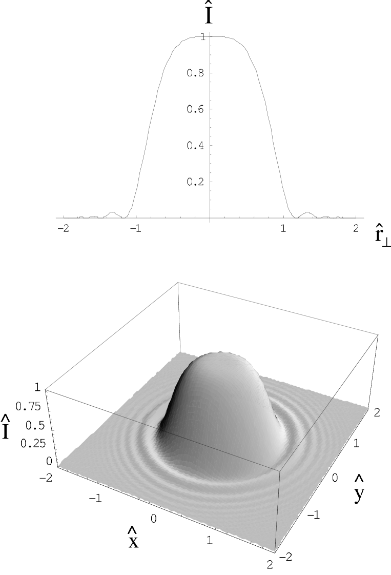
Figure 1: Normalized intensity distribution at the beam waist location, $\hat{I}$ as a function of $|\vec{\hat{r}}_{\bot}|$ (upper plot) and 3D view as a function of $\hat{x}$ and $\hat{y}$.

$$\vec{\hat{r}}_{\bot}=\sqrt{\frac{\omega}{L_{w}c}}\vec{r}_{\bot}~{},$$ (78)

$$\vec{\hat{\theta}}=\sqrt{\frac{\omega L_{w}}{c}}\vec{\theta}~{},$$ (79)

and

$${\hat{z}}=\frac{z}{L_{w}}~{}$$ (80)

Figure 2: Evolution of the intensity profile for undulator radiation according to Eq. (82) (solid lines) and comparison with the far field asymptotic $\mathrm{sinc}^{2}(\hat{\theta}^{2}/4)$ (dashed lines). The profiles according to Eq. (82) are shown as a function of angles at different observation distances $\hat{z}_{o}=0.6$, $\hat{z}_{o}=0.75$, $\hat{z}_{o}=1.0$ and $\hat{z}_{o}=4.0$.

we obtain the relative intensity at the virtual source

$$\hat{I}(0,\hat{r}_{\bot})=\frac{1}{\pi^{2}}\left[\pi-2\mathrm{Si}\left({\hat{r}_{\bot}^{2}}\right)\right]^{2}~{},$$ (81)

and at any distance $\hat{z}_{o}$, both in the near and in the far zone:

$$\hat{I}\left(\hat{z}_{o},\hat{\theta}\right)=\hat{z}_{o}^{2}\left|\mathrm{Ei}\left(\frac{i\hat{z}_{o}^{2}\hat{\theta}^{2}}{2\hat{z}_{o}-1}\right)-\mathrm{Ei}\left(\frac{i\hat{z}_{o}^{2}\hat{\theta}^{2}}{2\hat{z}_{o}+1}\right)\right|^{2}~{},$$ (82)

where $\hat{I}$ is defined as a normalized version of $|\tilde{E}_{\bot}|^{2}$ in normalized units. Note that we use the notation $\hat{\theta}=\hat{r}_{\bot}/\hat{z}_{o}$ in the near zone as well, because it is convenient, for future discussions, to present the intensity as in Eq. (82). Aside for scaling factor, the intensity profile in Eq. (81) can be detected by imaging the virtual plane with an ideal lens.

The relative intensity at the virtual source is plotted in Fig. 1. The evolution of the intensity profile at different positions after the exit of the undulator according to Eq. (82) is plotted, instead in Fig. 2.

To conclude, a single electron produces a laser-like radiation beam with a virtual source located in the center of the undulator whose transverse size is much larger than the radiation wavelength. Following OUR1 , Eq. (74) and Eq. (76) can be generalized to the case of a particle with a given offset $\vec{l}$ and deflection angle $\vec{\eta}$ with respect to the longitudinal axis. The far-zone field, Eq. (74), can be generalized to

$$\widetilde{{E}}_{\bot}\left(z_{o},\vec{\eta},\vec{l},\vec{\theta}\right) = -\frac{K\omega eL_{w}}{c^{2}z_{o}\gamma}A_{JJ}\exp\left[i\frac{\omega z_{o}}{2c}\theta^{2}\right]\exp\left[-i\frac{\omega}{c}\vec{\theta}\cdot\vec{l}\right]$$ (84)

$$\times\mathrm{sinc}\left[\frac{\omega L_{w}\left|\vec{\theta}-\vec{\eta}\right|^{2}}{4c}\right]~{},$$

while the expression for the field at virtual source, Eq. (76), is transformed to:

$$\widetilde{{E}}_{\bot}\left(0,\vec{\eta},\vec{l},r_{\bot}\right) = i\frac{K\omega e}{c^{2}\gamma}A_{JJ}\exp\left[i\frac{\omega}{c}\vec{\eta}\cdot\left(\vec{r}_{\bot}-\vec{l}\right)\right]\left[\pi-2\mathrm{Si}\left(\frac{\omega\left|\vec{r}_{\bot}-\vec{l}\right|^{2}}{L_{w}c}\right)\right].$$ (85)

The meaning of Eq. (84) and Eq. (LABEL:undurad5gg) is that offset and deflection of the single electron motion with respect to the longitudinal axis of the system result in offset and deflection of the waist plane. Computer codes (e.g. ZEMAX ZEMA , PHASE PHAS ), often referred to as wavefront propagation codes have been developed and are now standard tools used to carry out Fourier Optics-based calculations. For example ZEMAX can be used for single-particle field calculations. Once the virtual source Eq. (LABEL:undurad5gg) is specified, it can be used as an input for computer codes. This allows propagation of the virtual wavefront in the presence of a complicated setup, very much like it has been used as an input to Eq. (7) in the particularly simple case of free-space propagation. One may also deal with SR from a beam of ultrarelativistic electrons. For example, in the case of spontaneous (incoherent) SR, radiation produced by an electron beam in an undulator can be treated as an incoherent collection of laser beams with different offsets and deflections (i.e. by summing up the intensities of laser-like beams with different offsets and deflections).

5 Application 2. Edge radiation

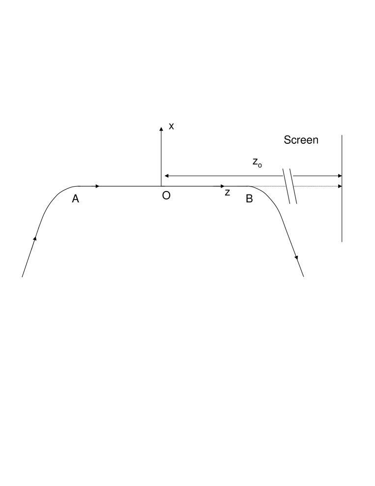
Figure 3: Edge radiation geometry. The beam enters the system through a bending magnet, passes a straight section and leaves the setup through another bend. Radiation is collected at a distance $z_{o}$ from the origin of the reference system, located in the middle of the straight section.

In this Section we apply the method described in Section 2 to the particular case of two dipole magnet edges.

We restrict ourselves to the system depicted in Fig. 3 and we consider a single particle moving along the system. The electron enters the setup via a bending magnet, passes through a straight section (segment $AB$) and exits the setup via another bend. Radiation is collected at a distance $z_{o}$ from the center of the reference system, located in the middle of the straight section. For wavelengths $\lambda\gg\lambda_{c}$, $\lambda_{c}$ being the critical wavelength of SR produced by bending magnets, the passage of the electron through the setup results in the emission of edge radiation (see, among the many references some early works and more recent developments in BOSF , CHUN , BOS4 , BOS7 , PROY , BOS2 , BOS3 , WILL and references therein).

In our case of study the trajectory and, therefore, the space integration in Eq. (23) can be split in three parts: the two bends, that will be indicated with $b_{1}$ and $b_{2}$, and the straight sections $AB$. One may write

$$\vec{\widetilde{{E}}}_{\bot}(z_{o},\vec{r}_{\bot o},\omega) = \vec{\widetilde{{E}}}_{b1}(z_{o},\vec{r}_{\bot o},\omega)+\vec{\widetilde{{E}}}_{AB}(z_{o},\vec{r}_{\bot o},\omega)+\vec{\widetilde{{E}}}_{b2}(z_{o},\vec{r}_{\bot o},\omega)~{},$$ (87)

with obvious meaning of notation.

We will denote the length of the segment $AB$ with $L$. This means that points $A$ and $B$ are located at longitudinal coordinates $z_{A}=-L/2$ and $z_{B}=L/2$.

First, with the help of Eq. (23) we will derive an expression for the field in the far zone. The intensity distribution in this case, result to be in agreement with expression in references cited above. Then, we will calculate the field distribution at the virtual source with the help of Eq. (17). Finally, Eq. (7) will allow us to find an expression for the field both in the near and in the far zone.

In the following we will only deal with a contribution of the electric field, i.e. that from the straight section.

According to the superposition principle, one should sum the contribution due to the straight section to that from the bends. In some cases one can ignore the presence of the bending magnets with good accuracy, and treat them as if they had zero length. In other cases one cannot do that. When one can neglect the field contribution due to the switchers, one can work in what can be called the ”zero-length switchers approximation”. While we direct the reader to Section 5.3 for details, we can mention here that for long enough straight sections $L\gg\gamma^{2}\lambdabar$, a condition for the zero-length switchers approximation to apply is $\lambda\gg\lambda_{c}$, $\lambda_{c}$ being the critical wavelength for SR from bends. Intuitively, magnets act like switchers: the first magnet switches the radiation harmonic on, the second switches it off. In the case depicted in Fig. 3 the switchers are bending magnets, but other setups can be considered where they have different physical realizations. For example, one may think of a setup where the phenomenon at study is the emission of bremsstrahlung in a collision between a ultra-relativistic electron and a nucleus. In this case, the switch-off process is taken care of by the collision itself. The nucleus plays the role of the switcher and the impact parameter, i.e. the minimal distance of the nucleus to the electron, characterizes the switcher itself. Note that there is no principle nor practical limitation to the length of the switcher. In the bremsstrahlung case we can assume that such length is very short, even with respect to the radiation wavelength. In the case of bends it can be much longer than all characteristic scales of interest, depending on the magnetic field strength, and all kind of intermediate situations can be realized. As one can see, the case of a straight line preceded and followed by switchers has a number of physical realizations. The only feature that different realizations must have in common by definition of switcher is that the switching process depends exponentially on the distance from the beginning of the process. Then, a characteristic length $d_{s}$ is associated to any switcher. Since electrodynamics is a linear theory, in the case when the contribution from the finite straight-line cannot be considered a good approximation of the total field, it can be considered as a building block for a more complicated setup. An example of a more sophisticated setup is studied in the next Section 6, where the problem of Transition Undulator Radiation is addressed.

In general, one can say that the problem of studying the field from a finite straight-line is of fundamental importance, independently of the type of switchers considered. This justifies our attention to the straight-section contribution to the field.

5.1 Far field pattern of edge radiation

5.1.1 Field contribution calculated along the straight section

Accounting for the geometry in Fig. 3 we have

$$s(z^{\prime})=z^{\prime}~{}~{}~{}~{}~{}\mathrm{for}~{}z_{A}<z^{\prime}<z_{B}~{}$$ (88)

With the help of Eq. (23) we write the contribution from the straight line $AB$ as

$$\vec{\widetilde{E}}_{AB}={i\omega e\over{c^{2}z_{o}}}\int_{-L/2}^{L/2}dz^{\prime}\exp{\left[i\Phi_{AB}\right]}\left(\theta_{x}{\vec{x}}+\theta_{y}{\vec{y}}\right)$$ (89)

where $\Phi_{AB}$ in Eq. (89) is given by

$$\Phi_{AB}=\omega\left[{\theta_{x}^{2}+\theta_{y}^{2}\over{2c}}z_{o}+{z^{\prime}\over{2c}}\left({1\over{\gamma^{2}}}+\theta_{x}^{2}+\theta_{y}^{2}\right)\right]~{},$$ (90)

$\theta_{x}=x_{o}/z_{o}$ and $\theta_{y}=y_{o}/z_{o}$ being the observation angles in the horizontal and vertical direction. From Eq. (89) one obtains

$$\vec{\widetilde{E}}_{AB} =\frac{i\omega eL}{c^{2}z_{o}}\exp\left[\frac{i\omega\theta^{2}z_{o}}{2c}\right]\vec{\theta}~{}\mathrm{sinc}\left[\frac{\omega L}{4c}\left(\theta^{2}+\frac{1}{\gamma^{2}}\right)\right]$$ (91)

where, as before

$$\theta^{2}=\theta_{x}^{2}+\theta_{y}^{2}~{}.$$ (92)

Eq. (91) is an exact expression for the electric field from the straight section $AB$. Note that Eq. (91) describes a spherical wave. Moreover, it explicitly depends on $L$ (this last remark will be useful later on).

The formation length $L_{\mathrm{fs}}$ for the straight section $AB$ can be written as

$$L_{\mathrm{fs}}\sim\min\left[\gamma^{2}\lambdabar,L\right]~{}.$$ (93)

Depending on the wavelength of interest then, $L_{\mathrm{fs}}\sim\gamma^{2}\lambdabar$ or $L_{\mathrm{fs}}\sim L$. In both cases, with the help of Eq. (90) we can give on a purely mathematical basis an upper limit to the value of the observation angle of interest related to the straight line:

$$\theta_{x,y}^{2}\lesssim\frac{\lambdabar}{L_{\mathrm{fs}}}~{}.$$ (94)

Note that, if $L_{\mathrm{fs}}\sim\gamma^{2}\lambdabar$, the maximal angle of interest is independent of the frequency.

Finally it should be remarked that the the far-zone asymptotic in Eq. (89) is valid at observation positions $z_{o}\gg L$. This is a necessary and sufficient condition for the vector $\vec{n}$ pointing from the retarded position of the source to the observer, to be considered constant. This result is independent of the formation length given by Eq. (93). Therefore, when $L\lesssim\gamma^{2}\lambdabar$ we can say that an observer is the far zone if and only if it is located many formation lengths away from the origin. This is no more correct when $L\gg\gamma^{2}\lambdabar$. In this case the observer can be located at a distance $z_{o}\gg\gamma^{2}\lambdabar$, i.e. many formation lengths away from the origin of the reference system, but still at $z_{o}\sim L$, i.e. in the near zone. As we see here, the formation length $L_{f}$ is often, but not always related with the definition of the far (or near) zone. This is the case for bending magnet radiation, but not for edge radiation. As has been remarked before in Section 3, the far (or near) is related with the characteristic size of the system $a$ (in our case $a=L$). In its turn $L_{f}\lesssim a$, which includes, as in the edge radiation case when $\gamma^{2}\lambdabar\ll L$, the situation $L_{f}\ll a$.

5.1.2 Energy spectrum of radiation

The radiation energy density as a function of angles and frequencies can be written as

$$\frac{dW}{d\omega d\Omega}=\frac{cz_{o}^{2}}{4\pi^{2}}\left|\vec{\widetilde{E}}\right|^{2}~{},$$ (95)

$d\Omega$ being the differential of the solid angle $\Omega$. Here we have used Parseval theorem and the fact that the irradiance (i.e. the energy per unit time per unit area, averaged over a period of the carrier frequency) is given by

$$P=\frac{c}{4\pi}\left<\left|{\vec{E}}\right|^{2}\right>=\frac{c}{2\pi}\left|\vec{\widetilde{E}}\right|^{2}~{},$$ (96)

where brackets $<...>$ denote averaging over a cycle of oscillation of the carrier wave. Substituting Eq. (91) in Eq. (95) it follows that

$$\frac{dW}{d\omega d\Omega}=\frac{\omega^{2}e^{2}L^{2}}{4\pi^{2}c^{3}}{\theta^{2}}~{}\mathrm{sinc}^{2}\left[\frac{\omega L}{4c}\left(\theta^{2}+\frac{1}{\gamma^{2}}\right)\right]~{}.$$ (97)

It is convenient to introduce normalized quantities

$$\vec{\hat{\theta}}=\sqrt{\frac{\omega L}{c}}\vec{\theta}~{},$$ (98)

$$\hat{\phi}=\frac{\omega L}{\gamma^{2}c}~{},$$ (99)

With Eq. (97) in mind and using normalized units, we may write the directivity diagram $\hat{I}$ of the radiation as

$$\hat{I}=\mathrm{const.}\times{\hat{\theta}^{2}}~{}\mathrm{sinc}^{2}\left[\frac{1}{4}\left(\hat{\theta}^{2}+\hat{\phi}\right)\right]$$ (100)

The directivity diagram in Eq. (100) is plotted in Fig. 4 for several values of $\hat{\phi}$ as a function of the normalized angle $\hat{\theta}$. The natural angular unit is evidently $(2\pi L/\lambda)^{-1/2}$.

Figure 4: Directivity diagram (solid lines) of the radiation from the setup in Fig. 3 for different values of $\hat{\phi}$. Dotted lines show the envelope of the directivity diagram.

There are two asymptotic cases for the problem parameter $\hat{\phi}$: $\hat{\phi}\ll 1$ and $\hat{\phi}\gg 1$. When $\hat{\phi}\gg 1$ the oscillating structures are fine with respect to the envelope of the directivity diagram. The intensity peaks where the envelope of the directivity diagram peaks, i.e. at $\hat{\theta}\sim\sqrt{\hat{\phi}}$. This feature for the far-field emission is shown in Fig. 4 for the case $\hat{\phi}=50$ and are typical for $\hat{\phi}\gg 1$. When the length of the straight section becomes smaller and $\hat{\phi}\ll 1$, we reach the other asymptotic limit. In this case, the period of the oscillations due to the $\sin(\cdot)$ function becomes much larger than $\sqrt{\hat{\phi}}$, as it can also be seen in Fig. 4 for the case $\hat{\phi}=0.1$. Then, the maximum intensity does not coincide anymore with the peak of the envelope of the directivity diagram, but it is found at $\hat{\theta}=2.2$.

The behavior of the far-field emission described here is well-known in literature, and has been first reported long ago in BOS4 . We take this as the starting point for further investigations based on Fourier Optics.

5.2 Method of virtual sources

5.2.1 Edge radiation as a field from a single virtual source

Eq. (17) and Eq. (91) allow one to characterize the virtual source through

$$\vec{\widetilde{E}}(0,\vec{r}_{\bot})=-\frac{\omega^{2}eL}{2\pi c^{3}}\int d\vec{\theta}~{}\vec{\theta}~{}\mathrm{sinc}\left[\frac{\omega L}{4c}\left(\theta^{2}+\frac{1}{\gamma^{2}}\right)\right]\exp\left[\frac{i\omega}{c}\vec{r}_{\bot}\cdot\vec{\theta}\right]~{}.$$ (101)

The Fourier transform in Eq. (101) is difficult to calculate analytically in full generality. However, simple analytical results can be found in the asymptotic case for $\hat{\phi}\ll 1$, i.e. for $2\pi L/(\gamma^{2}\lambda)\ll 1$. In this limit, the right hand side of Eq. (101) can be calculated with the help of polar coordinates. An analytic expression for the field amplitude at the virtual source can then be found and reads:

$$\vec{\widetilde{E}}(0,\vec{r}_{\bot})=\frac{4\omega e}{c^{2}L}\vec{r}_{\bot}\mathrm{sinc}\left(\frac{\omega}{Lc}\left|\vec{r}_{\bot}\right|^{2}\right)~{}.$$ (102)

It is useful to remark, for future use, that similarly to the far-field emission Eq. (91), also the non-normalized version of the field in Eq. (102) explicitly depend on $L$. This is true in general, for any value of $\hat{\phi}$. After definition of the normalized transverse position

$$\vec{\hat{r}}_{\bot}=\sqrt{\frac{\omega}{Lc}}\vec{r}_{\bot}~{}$$ (103)

the intensity distribution of the virtual source is given by

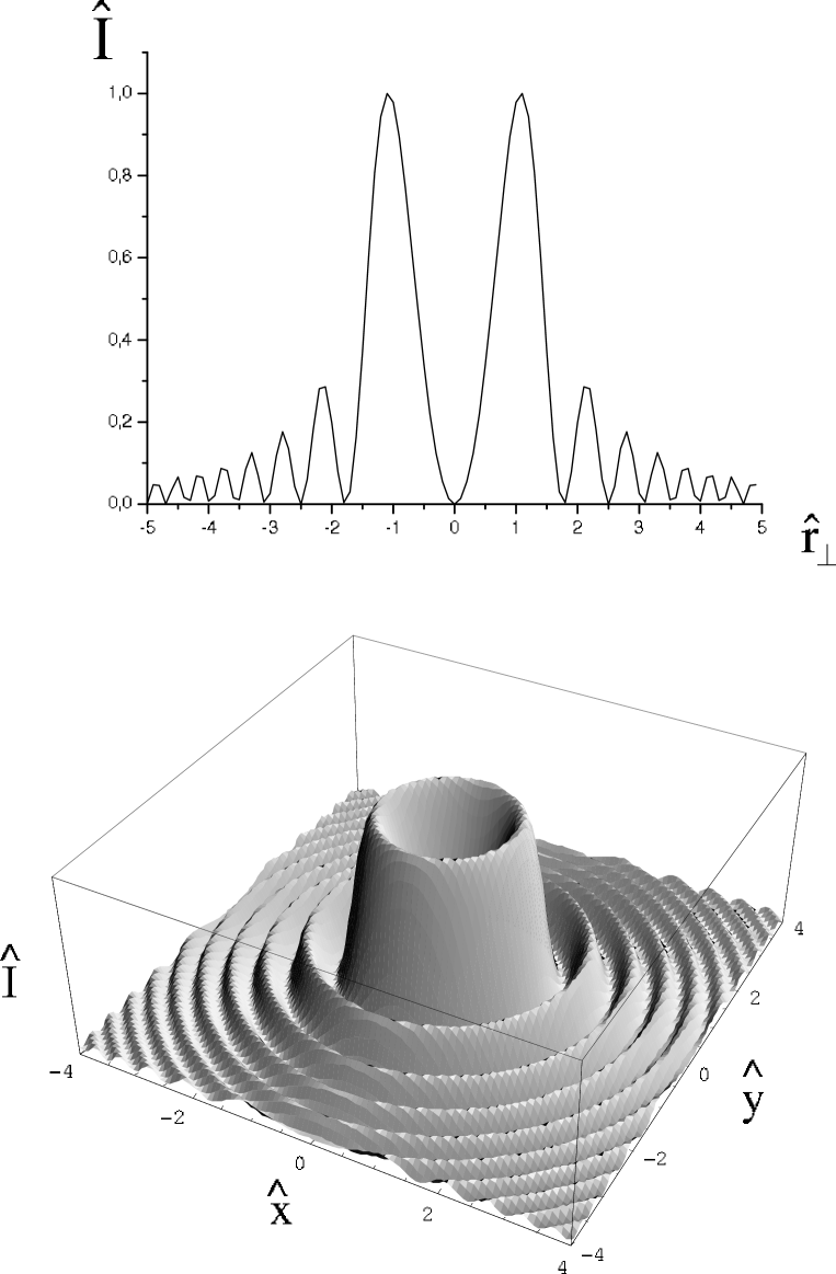
Figure 5: Intensity distribution at the virtual source, $\hat{I}$, as a function of $|\vec{\hat{r}_{\bot}}|$ (upper plot) and 3D view as a function of $\hat{x}$ and $\hat{y}$.

$$\hat{I}(\hat{r}_{\bot})=\mathrm{const.}\times{\hat{r}_{\bot}}^{2}\mathrm{sinc}^{2}\left({\hat{r}_{\bot}}^{2}\right)~{},$$ (104)

it can be detected (aside for scaling factors) by imaging the virtual plane with an ideal lens, and is plotted in Fig. 5.

Note that Eq. (102) describes a virtual source characterized by a plane wavefront. Application of the Fresnel propagation formula, Eq. (7) to Eq. (102) allows one to reconstruct the field both in the near and in the far region. We obtain the following result:

$$\vec{\widetilde{E}}({z}_{o},\vec{r}_{\bot}) =-\frac{2e}{c}\frac{\vec{{r}}_{\bot}}{{r}_{\bot}^{2}}\exp\left[i\frac{\omega{r}_{\bot}^{2}}{2c{z}_{o}}\right]$$ (106)

$$\times\left[\exp\left(-\frac{i\omega{r}_{\bot}^{2}}{2c{z}_{o}(1+2{z}_{o}/L)}\right)-\exp\left(\frac{i\omega{r}_{\bot}^{2}}{2c{z}_{o}(-1+2{z}_{o}/L)}\right)\right]~{}.$$

Eq. (106) solves the field propagation problem for both the near and the far field in the limit for $\hat{\phi}\ll 1$.

The intensity profile associated with Eq. (106) is given by

$${\hat{I}}(\hat{\theta}) = \frac{1}{\hat{\theta}^{2}}\left|\left[\exp\left(-\frac{i\hat{\theta}^{2}\hat{z}_{o}}{2(1+2\hat{z}_{o})}\right)-\exp\left(\frac{i\hat{\theta}^{2}\hat{z}_{o}}{2(-1+2\hat{z}_{o})}\right)\right]\right|^{2}~{},$$ (107)

where $\hat{\theta}=\hat{r}_{\bot}/\hat{z}_{o}$ and $\hat{z}_{o}=z_{o}/L$.

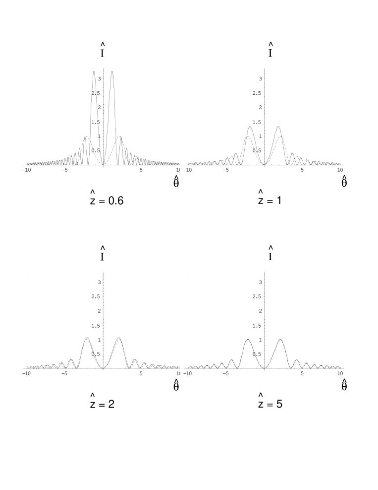
Figure 6: Evolution of the intensity profile for edge radiation in the limit for $\hat{\phi}\ll 1$. These profiles are shown as a function of angles at different observation distances $\hat{z}_{o}=0.6$, $\hat{z}_{o}=1.0$, $\hat{z}_{o}=2.0$ and $\hat{z}_{o}=5.0$ (solid lines). The dashed line always refers to the far-zone intensity.

In the limit for $\hat{z}_{o}\longrightarrow\infty$ Eq. (106) and Eq. (107) respectively transform to

$$\vec{\widetilde{E}} =\frac{i\omega eL}{c^{2}z_{o}}\exp\left[\frac{i\omega\theta^{2}z_{o}}{2c}\right]\vec{\theta}~{}\mathrm{sinc}\left[\frac{\omega L\theta^{2}}{4c}\right]$$ (108)

and

$$\hat{I}=\mathrm{const.}\times{\hat{\theta}^{2}}~{}\mathrm{sinc}^{2}\left[\frac{\hat{\theta}^{2}}{4}\right]~{},$$ (109)

corresponding to Eq. (91) and Eq. (100) in the asymptotic case for for $\hat{\phi}\ll 1$.

Note that when $\hat{\phi}\ll 1$ we have only two asymptotic regions with respect to $\hat{z}_{o}$: the far zone for $\hat{z}_{o}\gg 1$ and the near zone for $\hat{z}_{o}\ll 1$. Of course, it should be stressed that in the case $\hat{z}_{o}\ll 1$ we still hold the assumption that the approximation of zero-length switchers is satisfied. It is interesting to study the evolution of the intensity profile for edge radiation along the longitudinal axis. This gives an idea of how good the far field approximation ($\hat{z}_{o}\gg 1$) is. A comparison between intensity profiles at different observation points is plotted in Fig. 6.

The case $\hat{\phi}\ll 1$ studied until now corresponds to a short straight section $L\ll\gamma^{2}\lambdabar$. When this is condition is not satisfied, we find that the integral on the right hand side of Eq. (101) is difficult to calculate analytically. However, one can use numerical techniques. With the help of polar coordinates, the right hand side of Eq. (101) can be transformed in a one-dimensional integral, namely

Figure 7: Intensity profiles of the virtual source for the setup in Fig. 3. These profiles are shown for $\hat{\phi}=0.1$, $\hat{\phi}=1.0$, $\hat{\phi}=10.0$ and $\hat{\phi}=50.0$ (solid lines). Solid curves are calculated with the help of Eq. (110). The dotted lines show comparison with the asymptotic limit for $\hat{\phi}\ll 1$, shown in Fig. 5 and calculated using Eq. (104).

Figure 8: Intensity distribution at the virtual source for the setup in Fig. 3 for $\hat{\phi}=50$ (enlargement of the bottom right graph in Fig. 7).

$$\vec{\widetilde{E}}(0,\vec{r}_{\bot})=-\frac{4\omega e}{c^{2}}\frac{\vec{r}_{\bot}}{r_{\bot}}\int_{0}^{\infty}\frac{{\theta}^{2}}{{\theta}^{2}+1/\gamma^{2}}\sin\left[\frac{\omega L}{4c}\left(\theta^{2}+\frac{1}{\gamma^{2}}\right)\right]J_{1}\left(\frac{\omega{\theta}{r}_{\bot}}{c}\right)d{\theta}~{}.$$ (110)

We calculated the intensity distribution associated with the virtual source for values $\hat{\phi}=0.1$, $\hat{\phi}=1$, $\hat{\phi}=10$ and $\hat{\phi}=50$, corresponding to directivity diagrams in the far zone in Fig. 4. We plot these distributions in Fig. 7. In particular, it is instructive to make a separate, enlarged plot of the case $\hat{\phi}=50$, that is in the asymptotic case for $\hat{\phi}\gg 1$. This is given in Fig. 8. Fine structures are now evident, and are consistent with the presence of fine structures in Fig. 4 for the far zone. In fact, as we have seen, the field in the far region and the virtual source are linked, basically, by a Fourier transform. In principle, this allows to qualitatively describe the situation at the virtual source through the reciprocal relation. However, as we have said before, when $\hat{\phi}\gg 1$, in the far zone we have fine structures with variable width $\delta\theta$ (see also Fig. 4). As a result, in the limiting case $\hat{\phi}\gg 1$, use of the reciprocal relation to describe the properties of the virtual source is problematic. For example, a typical width $\delta\hat{\theta}\sim 1$ should correspond to typical dimension of the virtual source of order unity, that is in obvious disagreement with Fig. 8. Nonetheless, we managed to specified the field at the virtual source by means of numerical techniques, even in the case $\hat{\phi}\gg 1$ (see Fig. 8). Once the field at the virtual source is specified for any value of $\hat{\phi}$, Fourier Optics can be used to propagate it. In free space, the Fresnel formula must be used. However, we prefer to proceed in another way. There is, in fact, an alternative way to obtain the solution to the field propagation problem valid for any value of $\hat{\phi}$ and capable of giving a better physical insight for large values of $\hat{\phi}$.

5.2.2 Edge radiation as a superposition of the field from two virtual sources

Let us begin considering the far field in Eq. (91). This can also be written as

$$\vec{\widetilde{E}}\left({z}_{o},\vec{\theta}\right)=\vec{\widetilde{E}}_{1}\left({z}_{o},\vec{\theta}\right)+\vec{\widetilde{E}}_{2}\left({z}_{o},\vec{\theta}\right)~{}$$ (111)

where

$$\vec{\widetilde{E}}_{1,2}\left({z}_{o},\vec{\theta}\right)=\pm\frac{2e\vec{{\theta}}}{c{z}_{o}(\theta^{2}+1/\gamma^{2})}\exp\left[\pm\frac{i\omega L}{4c\gamma^{2}}\right]\exp\left[\frac{i\omega L\theta^{2}}{2c}\left(\frac{z_{o}}{L}\pm\frac{1}{2}\right)\right].$$ (112)

The two terms $\vec{\widetilde{E}}_{1}$ and $\vec{\widetilde{E}}_{2}$ represent two spherical waves respectively centered at ${z}=L/2$ and ${z}=-L/2$, that is at the edges of the straight section. Analysis of Eq. (112) shows that both contributions to the total field are peaked at an angle of order $1/\gamma$. While, as has been seen before, the total field in dimensional units explicitly depends on the straights section length $L$, the two expressions $\vec{\widetilde{E}}_{1}$ and $\vec{\widetilde{E}}_{2}$ exhibit dependence on $L$ through phase factors only. This fact will have interesting consequences, as we will discuss later. The two spherical waves represented by $\vec{\widetilde{E}}_{1}$ and $\vec{\widetilde{E}}_{2}$ may be thought as originating from two separate virtual sources located at the edges of the straight section. One may then describe the system with the help of two separate virtual sources, and interpret the field at any distance as the superposition of the contributions from two edges. This viewpoint is completely equivalent to that considered before involving a single virtual source in the straight line center. We are presenting here a different description of the same phenomenon. As we have seen before, we could not specify, analytically, the single virtual source in the center of the straight line. In contrast to this it is possible to specify the two virtual sources at the edges of the setup. In order to so so we take advantage of a slightly modified version of Eq. (17) that accounts for an arbitrary position of the source ${z}_{s(1,2)}$:

$$\vec{\widetilde{E}}\left({z}_{s(1,2)},\vec{r}_{\bot}\right) = \frac{i\omega{z}_{o}}{2\pi c}\int d\vec{\theta}$$ (114)

$$\times\exp{\left[-\frac{i\omega{\theta}^{2}}{2c}\left(z_{o}+{z}_{s(1,2)}\right)\right]}{\vec{\widetilde{E}}}_{1,2}\left({z}_{o},\vec{\theta}\right)\exp\left[\frac{i\omega}{c}\vec{r}_{\bot}\cdot\vec{\theta}\right]~{},$$

Separately substituting $\vec{\widetilde{E}}_{1}$ and $\vec{\widetilde{E}}_{2}$ into Eq. (LABEL:virfiesh2), and with the help of polar coordinates, we find the following expressions for the field at the virtual source positions ${z}_{s1}=L/2$ and ${z}_{s2}=-L/2$:

$$\vec{\widetilde{E}}\left(\pm\frac{L}{2},\vec{r}_{\bot}\right)=\mp\frac{2ie\omega}{c^{2}\gamma}\exp\left[\pm\frac{i\omega L}{4c\gamma^{2}}\right]\frac{\vec{r}_{\bot}}{r}K_{1}\left(\frac{\omega r_{\bot}}{c\gamma}\right)~{},$$ (116)

where $K_{1}(\cdot)$ is the modified Bessel function of the first order. Analysis of Eq. (116) shows a typical scale related to the sources dimension of order $c\gamma/\omega$ in dimensional units, corresponding to $1/\sqrt{\hat{\phi}}$ in normalized units. This is in agreement with the fact that both source contributions to the far field are peaked at an angle of order $\sqrt{\hat{\phi}}$. Note that this remark is only qualitative. The peak angle in the far zone does not correspond univocally to the width of the field distribution, nor the typical scale $1/\sqrt{\hat{\phi}}$ of the virtual sources can be univocally associated to the width of the sources. Also note that since the far zone field in dimensional units exhibit dependence on $L$ only through phase factors only has its counterpart in the fact that the field at the virtual sources, written in dimensional units, exhibit dependence on $L$ only through phase factors as well.

Application of the Fresnel formula allows to calculate the field at any distance ${z}_{o}$ in free space. Of course, Eq. (116) can also be used as input to any Fourier code to calculate the field evolution in the presence of whatever optical beamline. However, we restrict ourselves to the free-space case. Taking advantage, once more, of polar coordinates and using the definition $\vec{\hat{\theta}}=\vec{\hat{r}}_{\bot}/\hat{z}_{o}$ we obtain the following scaling law for the intensity in normalized units:

$$\hat{I}\left(\hat{z}_{o},\vec{\hat{\theta}}\right) = \mathrm{const}\cdot\left|\left\{-\frac{\vec{\hat{\theta}}}{\hat{\theta}}\frac{2i\sqrt{\hat{\phi}}\exp\left[i\hat{\phi}/4\right]}{\hat{z}_{o}-1/2}\exp\left[\frac{i\hat{\theta}^{2}\hat{z}_{o}^{2}}{2\left(\hat{z}_{o}-1/2\right)}\right]\right.\right.$$ (120)

$$\left.\left.\times\int_{0}^{\infty}d\hat{r}^{\prime}_{\bot}\hat{r}^{\prime}_{\bot}K_{1}\left(\sqrt{\hat{\phi}}\hat{r}^{\prime}_{\bot}\right)J_{1}\left(\frac{\hat{\theta}\hat{r}^{\prime}_{\bot}\hat{z}_{o}}{\hat{z}_{o}-1/2}\right)\exp\left[\frac{i\hat{r}_{\bot}^{{}^{\prime}2}}{2\left(\hat{z}_{o}-1/2\right)}\right]\right\}\right.$$

$$\left.+\left\{\frac{\vec{\hat{\theta}}}{\hat{\theta}}\frac{2i\sqrt{\hat{\phi}}\exp\left[-i\hat{\phi}/4\right]}{\hat{z}_{o}+1/2}\exp\left[\frac{i\hat{\theta}^{2}\hat{z}_{o}^{2}}{2\left(\hat{z}_{o}+1/2\right)}\right]\right.\right.$$

$$\left.\left.\times\int_{0}^{\infty}d\hat{r}^{\prime}_{\bot}\hat{r}^{\prime}_{\bot}K_{1}\left(\sqrt{\hat{\phi}}\hat{r}^{\prime}_{\bot}\right)J_{1}\left(\frac{\hat{\theta}\hat{r}^{\prime}_{\bot}\hat{z}_{o}}{\hat{z}_{o}+1/2}\right)\exp\left[\frac{i\hat{r}_{\bot}^{{}^{\prime}2}}{2\left(\hat{z}_{o}+1/2\right)}\right]\right\}\right|^{2}~{}.$$

In the limit for $\hat{z}_{o}\gg 1$ Eq. (LABEL:fipr) gives back the square modulus of Eq. (112) in normalized units. Similarly, in the limit for $\hat{\phi}\ll 1$, and using the fact that $K_{1}(\sqrt{\hat{\phi}}\hat{r}_{\bot})\simeq 1/(\hat{r}_{\bot}\sqrt{\hat{\phi}})$ one recovers the square modulus of Eq. (106). In general, the integrals in Eq. (LABEL:fipr) cannot be calculated analytically, but they can be integrated numerically.

Figure 9: Intensity profile for edge radiation for $\hat{\phi}=50$. These profiles are shown as a function of angles at different observation distances $\hat{z}_{o}=0.52$, $\hat{z}_{o}=0.6$, $\hat{z}_{o}=1.5$ and $\hat{z}_{o}=100.0$.

First we checked that we are able to recover, posing $\hat{z}_{o}=0$, the intensity profile for the single virtual source, already calculated numerically and shown in Fig. 7 and Fig. 8. Then we propagated the field at non-virtual positions, for $\hat{z}_{o}>1/2$. In Fig. 9 we plotted, in particular, results for the propagation in case $\hat{\phi}=50$. Radiation profiles are shown as a function of angles $\hat{\theta}$ at different observation distances $\hat{z}_{o}=0.52$, $\hat{z}_{o}=0.6$, $\hat{z}_{o}=1.5$ and $\hat{z}_{o}=100.0$.

From a technical viewpoint, it is easier to deal with two sources than with one, because the expression for the virtual two sources is analytical, whereas that for a single one is not. Moreover, as said before, the two-sources picture gives new physical insight for the asymptotic limit $\hat{\phi}\gg 1$.

Qualitatively, we can deal with two limiting cases of the theory, the first for $\hat{\phi}\ll 1$ and the second for $\hat{\phi}\gg 1$.

Let us first discuss the case $\hat{\phi}\ll 1$. The field at any observation distance is given by Eq. (106). There are only two observation zones of interest.

• Far zone. In the limit for $\hat{z}_{o}\gg 1$ one has the far field Eq. (108).

• Near zone. When $\hat{z}_{o}\lesssim 1$ instead, one has the near field Eq. (106).

As it can be seen from Eq. (106), the total field is given, both in the near and in the far zone, by the interference of the two virtual sources located at the straight section edges. Eq. (LABEL:fipr) shows that the transverse dimension of these virtual sources is given by $\gamma\lambdabar$ in dimensional units. This is the typical scale in $r^{\prime}_{\bot}$ after which the integrands in $d\hat{r}^{\prime}_{\bot}$ in Eq. (LABEL:fipr) are suppressed by the function $K_{1}$. Thus, the sources at the edges of the straight section have a dimension that is independent of $L$. In the center of the setup instead, the virtual source has a dimension of order $\sqrt{\lambdabar L}$ as it can be seen Eq. (104). When $\hat{\phi}\ll 1$ the source in the center of the setup is much smaller than those at the edge. This looks paradoxical. The explanation is that the two contributions due to edge sources interfere in the center of the setup. In particular, when $\hat{\phi}\ll 1$ they nearly compensate, as they have opposite sign. As a result of this interference, the single virtual source in the center of the setup (and its far-zone counterpart) has a dimension dependent on $L$ (in non-normalized units) while at the edges (and in their far-zone counterpart) the dependence on $L$ is limited to phase factors only. Due to the fact that edges contributions nearly compensate for $\hat{\phi}\ll 1$ one may say that the single-source picture is particularly natural in the case $\hat{\phi}\ll 1$.

Let us now discuss the case $\hat{\phi}\gg 1$. In this situation the two-sources picture becomes more natural. Let us define with ${d}_{1,2}={z}_{o}\mp L/2$ the distances of the observer from the edges. As seen before, the transverse dimension of the sources at the edges of the straight section is $r^{\prime}_{\bot}\sim\gamma\lambdabar$. Moreover, we see from Eq. (89) and Eq. (90) that when $\hat{\phi}\gg 1$ the formation length is $L_{f}=\gamma^{2}\lambdabar$, much shorter than the system dimension $L$. As a result, one can recognize four regions of interest, that are more naturally discussed in the two-source picture.

• Two-edge radiation. Far zone. When $d_{1,2}\gg L$ we are summing far field contributions from the two edge sources. This case is well represented in Fig. 9 for $\hat{z}_{o}=100$, where interference effects between the two edges contribution are well visible.

• Two-edge radiation. Near zone. When $d_{1,2}\sim L$ the observer is located far away with respect to the formation length of the sources $L^{\prime}_{f}$. Both contributions from the sources are important, but that from the nearest source begins to become the main one, as $d_{1}$ and $d_{2}$ become sensibly different. This case is well represented in Fig. 9 for $\hat{z}_{o}=1.5$.

• Single-edge radiation. Far zone. When $\gamma^{2}\lambdabar\ll d_{1}\ll L$ the contribution due to the near edge is dominant, while the far edge contribution is negligible. Such tendency is clearly depicted in Fig. 9 for $\hat{z}_{o}=0.6$. Interference tends to disappear as the near edge becomes the dominant one, while the intensity distribution tends to approximate

  $${I}\left({\theta}\right)=\mathrm{const}\times\left|\vec{\widetilde{E}}_{2}\left(z_{o},\theta\right)\right|^{2}=\mathrm{const}\times\frac{4e^{2}}{c^{2}z_{o}^{2}}\frac{\gamma^{4}{\theta}^{2}}{\left(\gamma^{2}\theta^{2}+1\right)^{2}}~{},$$ (122)

  where $\vec{\widetilde{E}}_{2}$ is the single edge far field limit in Eq. (112).

• Single-edge radiation. Near zone. When $0<d_{1}\lesssim\gamma^{2}\lambdabar$ we have the near-field contribution from a single edge. As ${d}_{1}$ becomes smaller and smaller the intensity distribution tends to reproduce the singular behavior from a single virtual source, i.e. the square modulus of Eq. (116):

  $${I}\left(\frac{L}{2},\vec{r}_{\bot}\right)=\mathrm{const}\times\left|\vec{\widetilde{E}}\left(\frac{L}{2},\vec{r}_{\bot}\right)\right|^{2}=\mathrm{const}\times\frac{4e^{2}}{\gamma^{2}\lambdabar^{2}c^{2}}\left|K_{1}\left(\frac{r_{\bot}}{\gamma\lambdabar}\right)\right|^{2}~{}.$$ (123)

  This tendency can be seen in Fig. 9 for $\hat{z}_{o}=0.52$.

It should be noted that the straight section contribution has been calculated within the applicability region of the paraxial approximation, but independently of all assumptions on the switchers. If switchers or other setup parts are present, their contribution must be separately calculated and added to the contribution due to the straight section. For instance, if an observer is placed after a switcher located downstream of the straight section, the field due to the straight section has physical meaning (i.e. the theoretical intensity can be compared with experiment) only if the zero-length switchers approximation can be applied. Otherwise it is just a mathematically convenient term, a partial result to be summed with the switcher contribution. If, instead, the observer is placed on a transverse plane placed before the switcher, at the downstream edge of the straight section, the switcher (or any other part of the setup following the straight section) will not influence the field with ultra-relativistic accuracy. Eq. (116) (or Eq. (123)) can then be compared with experimental results. As has been discussed in footnote 13, the singularity in the field at $r_{\bot}=0$ is fundamentally related with our ignorance about the structure of the electron.

It should be noted that our Eq. (116) is identical to the frequency-domain expression for the transverse component of the field originating from an ultra-relativistic electron moving with constant velocity (see JACK ). In fact, our treatment for the straight-section contribution in the case of single-edge radiation in the near zone gives, within an accuracy of $1/\gamma^{2}$, the same result found in JACK for bremsstrahlung in a collision between an ultra-relativistic electron and an atomic nucleus by means of the method of virtual quanta. In the bremsstrahlung case the electron harmonic is switched off within a length $d_{s}\ll\lambdabar$ even in the model for an electron on a uniform motion, because non-negligible contributions to the field are generated by the part of the trajectory before the nucleus only, while the trajectory after the nucleus gives negligible contribution within an accuracy $1/\gamma^{2}$. Exact calculation, retaining all parts of the Lienard-Wiechert field show that the field from the relativistic particle is equivalent to two virtual pulses of radiation. One moves longitudinally, i.e. in the same direction as the electron. A second moves transversely, i.e. perpendicularly with respect to the electron direction. As already said, the component of the frequency spectrum due to the longitudinal pulse is given by our Eq. (116). At any observation position, the component due to the transverse pulse can be neglected with an accuracy $1/\gamma^{2}$. In other words, the weak transverse pulse is a correction to the main longitudinal pulse. It may be interpreted as an evanescent wave decaying in the longitudinal direction, since it propagates transversely, i.e. at large angle $\pi/2$ with respect to the $z$ axis. Dropping this term gives back our result, that was found in the paraxial approximation.

Our previous result in Eq. (116) constitutes a novel finding in theory of edge radiation dealing with the situation of a particle in straight motion. The case of a particle in straight motion is of fundamental importance, because of two reasons. First, our result can be applied to any setup where the zero-length switchers approximation applied. Second, straight sections are basic building blocks for any magnetic setup, and our expression for the near field from a straight section can be used, as part of the total field, also in the case when the zero-length switchers approximation fails.

5.3 Supplementary remarks on the zero-length switcher approximation

For the sake of completeness it remains to qualitatively discuss the conditions when the field due to switchers is negligible, because in this case one can work in the ”zero-length switchers approximation”. We consider the case when switchers are present in the form of bending magnets. In particular, here we report results from an analysis of the problem in the limit $L\gg\gamma^{2}\lambdabar$. In this case the formation length associated with the straight section is given by $\gamma^{2}\lambdabar$, while the formation length associated with the bending magnet is given by $(\lambdabar\rho^{2})^{1/3}$, $\rho$ being the radius of the bend. The ratio between the latter and the former is indicated with $\epsilon^{2}=(\lambda_{c}/\lambda)^{2/3}\ll 1$, where $\lambda_{c}=4\pi\rho/(3\gamma^{3})$ is the critical wavelength for SR from the bend and we assumed $\lambda\gg\lambda_{c}$, as we are interested in edge radiation. The product between the small quantity $\epsilon$ and the formation length for the straight section is indicated with $d_{c}=\epsilon\gamma^{2}\lambdabar$, and turns out to constitute an extra characteristic-length for our system. Let us indicate with $d$ the distance between a transverse plane of observation and the downstream edge of the straight section. At very short distances, for $d\ll d_{c}$, the straight section contribution dominates the bending magnet one for transverse displacements from the $z$-axis $r_{\bot}$ of order $r_{\bot}>\epsilon\gamma\lambdabar$. Within the area $r_{\bot}<\epsilon\gamma\lambdabar$ the two contributions are comparable. Note that in this area the contribution from the straight section is much larger than in the area for $\epsilon\gamma\lambdabar<r_{\bot}<\gamma\lambdabar$ due to singular behavior of the field contribution from the straight section at $r_{\bot}\longrightarrow 0$. When $d\sim d_{c}$ the zero-length switcher approximation cannot be used, and contributions from the bend should be calculated explicitly. When $\gamma^{2}\lambdabar\gtrsim d\gg d_{c}$ we have room for direct application of our theory for the straight section within the range $0<r_{\bot}\ll(\lambdabar^{2}\rho)^{1/3}$, because the characteristic size of the radiation is $\epsilon(\lambdabar^{2}\rho)^{1/3}$. Finally, for $d\gg\gamma^{2}\lambdabar$, we have room for direct application of our theory for the straight section within the angular range $0<\theta\ll(\lambdabar/\rho)^{1/3}$, because the characteristic angle of the radiation is $\epsilon(\lambdabar/\rho)^{1/3}$.

6 A more sophisticated application. Transition undulator radiation

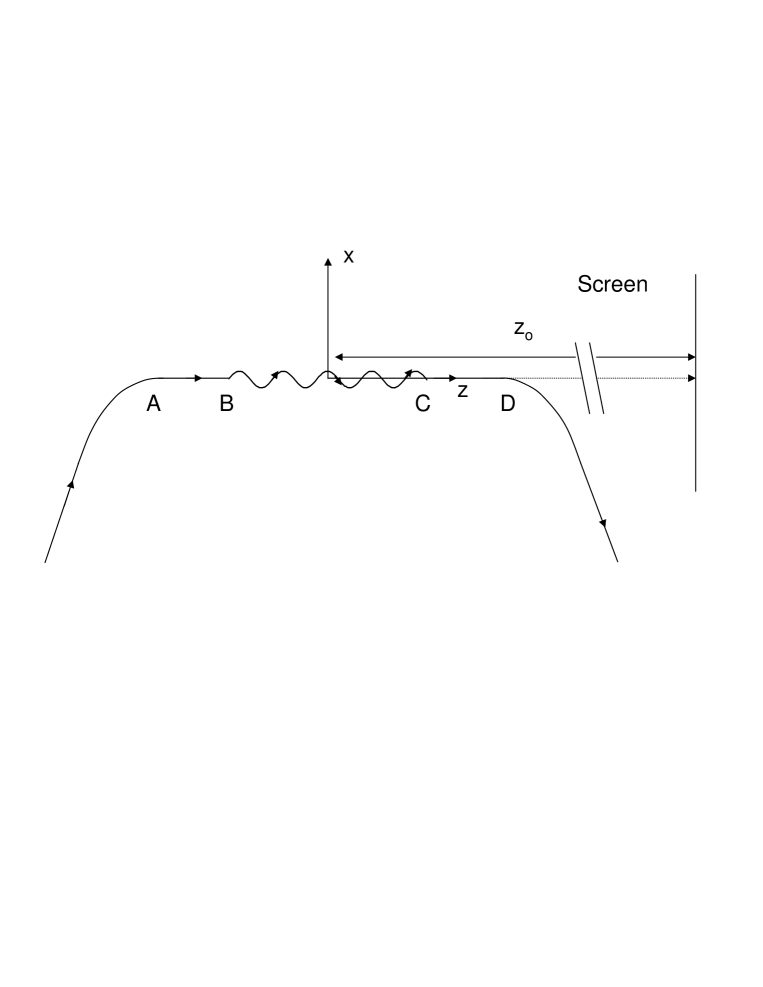
Figure 10: Edge radiation geometry. The beam enters the system through a bending magnet, passes a straight section, an undulator and another straight section before leaving the setup through another bend. Radiation is collected at a distance $z_{o}$ from the origin of the reference system, located in the middle of the undulator.

In this Section we apply the method described in Section 2 to the more complicated case of an undulator setup.

Instead of the setup in Fig. 3, we now consider the system depicted in Fig. 10 and we consider a single particle moving along the system. The electron enters the setup via a bending magnet, passes through a straight section (segment $AB$), an undulator (segment $BC$), and another straight section (segment $CD$). Finally, it exit the setup via another bend. Radiation is collected at a distance $z_{o}$ from the center of the reference system, located in the middle of the undulator. The passage of the electron through the setup results in collimated emission of radiation in the low photon energy range, a mechanism analogous to transition radiation. This kind of radiation is known in literature as TUR KIM1 , BOS4 , KINC , CAST , BOS6 , ROY2 , even though in this paper we prefer to denote it as edge radiation from undulator setup.

In our case of study the trajectory and, therefore, the space integration in Eq. (23) can be split in five parts: the two bends, that will be indicated with $b_{1}$ and $b_{2}$, the two straight sections $AB$ and $CD$ and the undulator $BC$. One may write

$$\vec{\widetilde{{E}}}_{\bot}(z_{o},\vec{r}_{\bot o},\omega) = \vec{\widetilde{{E}}}_{b1}(z_{o},\vec{r}_{\bot o},\omega)+\vec{\widetilde{{E}}}_{AB}(z_{o},\vec{r}_{\bot o},\omega)+\vec{\widetilde{{E}}}_{BC}(z_{o},\vec{r}_{\bot o},\omega)$$ (125)

$$+\vec{\widetilde{{E}}}_{CD}(z_{o},\vec{r}_{\bot o},\omega)+\vec{\widetilde{{E}}}_{b2}(z_{o},\vec{r}_{\bot o},\omega)~{},$$

with obvious meaning of notation.

We will denote the length of the segment $AD$ with $L_{\mathrm{tot}}$, while we will indicate the length of the straight section $AB$ with $L_{1}$, the length of the straight section $CD$ with $L_{2}$ and the length of the undulator with $L_{w}$. It follows

$$L_{\mathrm{tot}}=L_{1}+L_{w}+L_{2}~{}.$$ (126)

This means that point $A$ is located at longitudinal coordinate $z_{A}=-L_{1}-L_{w}/2$, while $B$, $C$ and $D$ are located respectively at $z_{B}=-L_{w}/2$, $z_{C}=L_{w}/2$ and $z_{D}=L_{w}/2+L_{2}$.

First, with the help of Eq. (23) we will derive an expression for the field in the far zone. The intensity distribution in this case, results to be in agreement with that given in BOS4 . Then, we will calculate the field distribution at the virtual source with the help of Eq. (17). Finally, Eq. (7) will allow us to find an expression for the field both in the near and in the far zone. We will the turn to analyze the case when a undulator is present, and describe the field from the setup as superposition of three laser-like beam from straight sections and undulator. In the following we will ignore the presence of the bending magnets, i.e. the radiation switchers. As before, we will treat them as if they had zero length. As a result, Eq. (125) can be simplified to

$$\vec{\widetilde{{E}}}_{\bot}(z_{o},\vec{r}_{\bot o},\omega) = \vec{\widetilde{{E}}}_{AB}(z_{o},\vec{r}_{\bot o},\omega)+\vec{\widetilde{{E}}}_{BC}(z_{o},\vec{r}_{\bot o},\omega)+\vec{\widetilde{{E}}}_{CD}(z_{o},\vec{r}_{\bot o},\omega)~{}.$$ (127)

We already addressed the question of the applicability region of the ”zero-length switcher approximation” in previous Section 5.

6.1 Far field from the undulator setup

Let us describe the far field from the undulator setup in Fig. 10 by separately characterizing the field contributions along undulator, straight sections and bends and finally adding them together.

6.1.1 Field contribution calculated along the undulator

We first consider the contribution $\vec{\widetilde{{E}}}_{BC}$ from the undulator, following OUR1 . Assuming a planar undulator we write the following expression for the transverse velocity of an electron:

$$\vec{v}_{\bot}(z^{\prime})=-{cK\over{\gamma}}\sin{\left(k_{w}z^{\prime}\right)}\vec{x}~{},$$ (128)

that is Eq. (72). Here $K$ is the undulator parameter defined in Eq. (71). Moreover, $k_{w}=2\pi/\lambda_{w}$, where $\lambda_{w}$ is the undulator period, so that the undulator length is $L=N_{w}\lambda_{w}$. The transverse position of the electron is therefore

$$\vec{r^{\prime}}_{\bot}(z^{\prime})=\frac{K}{\gamma k_{w}}\cos{\left(k_{w}z^{\prime}\right)}\vec{x}~{}.$$ (129)

An expression for the curvilinear abscissa $s$ as a function of the longitudinal position $z^{\prime}$ is given by

$$s(z^{\prime})={\frac{\beta}{\beta_{av}}}z^{\prime}-{K^{2}\over{8\gamma^{2}k_{w}}}\sin\left(2k_{w}z^{\prime}\right)~{},$$ (130)

where $\beta_{av}$ is the time-averaged velocity along the $z$ direction, that can be expressed as:

$$\beta_{av}=\beta\left(1-{K^{2}\over{4\gamma^{2}}}\right)~{}.$$ (131)

We can now substitute Eq. (129) and Eq. (128) in Eq. (23). Such substitution leads to a general expression, valid for any observer distance $z_{o}$. It is possible to obtain, similarly to many SR textbooks, a simplified expression valid in the limit for large values of $z_{o}$. Since we are interested in the contribution of the undulator device to the total field at the observer position, we will integrate Eq. (23) only along the undulator. Then all terms in $(z_{o}-z^{\prime})^{-1}$ in the phase factor of Eq. (23) can be expanded around $z_{o}$. In the far field limit we can retain first order terms in $z^{\prime}$. Dropping negligible terms we obtain

$$\vec{\widetilde{{E}}}_{BC}(z_{o},\vec{r_{\bot o}},\omega) = \frac{i\omega e}{c^{2}z_{o}}\int_{z_{B}}^{z_{C}}dz^{\prime}{\exp{\left[i\Phi_{BC}\right]}}\left\{\left[{K\over{\gamma}}\sin\left(k_{w}z^{\prime}\right)+\theta_{x}\right]{\vec{x}}+\theta_{y}{\vec{y}}\right\},$$ (132)

where

$$\Phi_{BC} = {\omega}\left\{{\theta_{x}^{2}+\theta_{y}^{2}\over{2c}}z_{o}+\frac{z^{\prime}}{2c}\left(\frac{1}{\gamma_{z}^{2}}+\theta_{x}^{2}+\theta_{y}^{2}\right)-\frac{K\theta_{x}}{\gamma k_{w}c}\cos(k_{w}z^{\prime})\right.$$ (134)

$$\left.-\frac{K^{2}}{8\gamma^{2}k_{w}c}\sin(2k_{w}z^{\prime})\right\}~{}.$$

The longitudinal Lorentz factor $\gamma_{z}$ in Eq. (134) is defined by

$$\gamma_{z}=\frac{\gamma}{\sqrt{1+{K^{2}}/{2}}}$$ (135)

and is always smaller than $\gamma$, because the average longitudinal velocity of the electron inside the undulator is smaller than that along the straight sections.

In this paper we will be interested up to frequencies much lower than the resonance frequency, i.e. $\omega\ll 2\gamma_{z}^{2}ck_{w}$. Then, the contribution due to the term in $\sin(k_{w}z^{\prime})$ in Eq. (132) can always be neglected when compared with the maximal field magnitude of the terms in $\theta_{x,y}$. Similarly, in Eq. (134), phase terms in $\cos(k_{w}z^{\prime})$ and $\sin(2k_{w}z^{\prime})$ can can also be neglected. As a result, Eq. (132) can be simplified as

$$\vec{\widetilde{{E}}}_{BC}(z_{o},\vec{r_{\bot o}},\omega) = \frac{i\omega e}{c^{2}z_{o}}\int_{z_{B}}^{z_{C}}dz^{\prime}{\exp{\left[i\Phi_{BC}\right]}}\left(\theta_{x}{\vec{x}}+\theta_{y}{\vec{y}}\right)$$ (136)

while

$$\Phi_{BC} = {\omega}\left[{\theta_{x}^{2}+\theta_{y}^{2}\over{2c}}z_{o}+\frac{z^{\prime}}{2c}\left(\frac{1}{\gamma_{z}^{2}}+\theta_{x}^{2}+\theta_{y}^{2}\right)\right]~{}.~{}$$ (137)

Finally, note that within these approximations, the curvilinear abscissa $s$ in Eq. (130) can be simplified to

$$s(z^{\prime})={\frac{\beta}{\beta_{av}}}z^{\prime}~{}.$$ (138)

6.1.2 Field contribution calculated along the straight sections

Let us now calculate the curvilinear abscissa along segments $AB$ and $CD$. Eq. (138) implies that the curvilinear abscissa at the undulator edges $z^{\prime}=\pm L_{w}/2$ is given by $\pm\beta L_{w}/(2\beta_{av})$. Moreover the curvilinear abscissa must be of the form $s(z^{\prime})=z^{\prime}+\mathrm{const.}$, because segments $AB$ and $CD$ are straight lines. It follows that

$$s(z^{\prime})=z^{\prime}+\frac{L_{w}}{2}\left(1-\frac{\beta}{\beta_{av}}\right)\simeq z^{\prime}+\frac{L_{w}}{4\gamma^{2}}-\frac{L_{w}}{4\gamma_{z}^{2}}~{}~{}~{}~{}~{}\mathrm{for}~{}z_{A}<z^{\prime}<z_{B}~{}$$ (139)

and

$$s(z^{\prime})=z^{\prime}-\frac{L_{w}}{2}\left(1-\frac{\beta}{\beta_{av}}\right)\simeq z^{\prime}-\frac{L_{w}}{4\gamma^{2}}+\frac{L_{w}}{4\gamma_{z}^{2}}~{}~{}~{}~{}~{}\mathrm{for}~{}z_{C}<z^{\prime}<z_{D}~{},$$ (140)

where we have used the fact that

$$\frac{1}{\beta_{av}}\simeq 1+\frac{1}{2\gamma_{z}^{2}}~{}.$$ (141)

With the help of Eq. (23) we write the contribution from the straight line $AB$ as

$$\vec{\widetilde{E}}_{AB}={i\omega e\over{c^{2}z_{o}}}\int_{z_{A}}^{z_{B}}dz^{\prime}\exp{\left[i\Phi_{AB}\right]}\left(\theta_{x}{\vec{x}}+\theta_{y}{\vec{y}}\right)$$ (142)

where $\Phi_{AB}$ in Eq. (142) is given by

$$\Phi_{AB}=\omega\left[{\theta_{x}^{2}+\theta_{y}^{2}\over{2c}}z_{o}-\frac{L_{w}}{4c\gamma_{z}^{2}}+\frac{L_{w}}{4c\gamma^{2}}+{z^{\prime}\over{2c}}\left({1\over{\gamma^{2}}}+\theta_{x}^{2}+\theta_{y}^{2}\right)\right]~{},$$ (143)

$\theta_{x}=x/z_{o}$ and $\theta_{y}=y/z_{o}$ being the observation angles in the horizontal and vertical direction. Note that we also used $v\simeq c$ when calculating the term ${L_{w}}/{(4c\gamma_{z}^{2})}$ in Eq. (143). The contribution from the straight line $CD$ is similar to that from the straight line $AB$ and reads

$$\vec{\widetilde{E}}_{CD}={i\omega e\over{c^{2}z_{o}}}\int_{z_{C}}^{z_{D}}dz^{\prime}\exp{\left[i\Phi_{CD}\right]}\left(\theta_{x}{\vec{x}}+\theta_{y}{\vec{y}}\right)$$ (144)

where $\Phi_{CD}$ in Eq. (144) is given by

$$\Phi_{CD}=\omega\left[{\theta_{x}^{2}+\theta_{y}^{2}\over{2c}}z_{o}+\frac{L_{w}}{4c\gamma_{z}^{2}}-\frac{L_{w}}{4c\gamma^{2}}+{z^{\prime}\over{2c}}\left(\frac{1}{\gamma^{2}}+\theta_{x}^{2}+\theta_{y}^{2}\right)\right]~{}.$$ (145)

In general, the phases $\Phi_{CD}$ and $\Phi_{AB}$ start exhibiting oscillatory behavior when $\omega z^{\prime}/(2c\gamma^{2})\sim 1$, which gives a maximal integration range in the longitudinal direction. Similarly as before, in general one has that the formation lengths $L_{\mathrm{fs1}}$ and $L_{\mathrm{fs2}}$ for the straight sections $AB$ and $CD$ can be written as

$$L_{\mathrm{fs(1,2)}}\sim\min\left[\lambda\gamma^{2},L_{(1,2)}\right]~{}.$$ (146)

Depending on the wavelength of interest then, $L_{\mathrm{fs(1,2)}}\sim\lambda\gamma^{2}$ or $L_{\mathrm{fs(1,2)}}\sim L_{(1,2)}$.

6.1.3 Total field and energy spectrum of radiation

Consider Eq. (127). The contributions for segment $AB$ and segment $CD$ are given by Eq. (142) and Eq. (144). One obtains

$$\vec{\widetilde{E}}_{AB} =-\frac{2e\left(\theta_{x}\vec{x}+\theta_{y}\vec{y}\right)}{\left(1/\gamma^{2}+\theta_{x}^{2}+\theta_{y}^{2}\right)cz_{o}}\exp\left[i\omega{\theta_{x}^{2}+\theta_{y}^{2}\over{2c}}z_{o}\right]\exp\left[-\frac{i\omega L_{w}}{4c\gamma_{z}^{2}}+\frac{i\omega L_{w}}{4c\gamma^{2}}\right]$$ (149)

$$\times\left\{\exp\left[-i\frac{\omega(L_{1}+L_{w}/2)}{2c}\left(\frac{1}{\gamma^{2}}+\theta_{x}^{2}+\theta_{y}^{2}\right)\right]\right.$$

$$\left.-\exp\left[-i\frac{\omega L_{w}}{4c}\left(\frac{1}{\gamma^{2}}+\theta_{x}^{2}+\theta_{y}^{2}\right)\right]\right\}$$

that can also be written as

$$\vec{\widetilde{E}}_{AB} =\frac{i\omega eL_{1}}{c^{2}z_{o}}\vec{\theta}\mathrm{sinc}\left[\frac{\omega L_{1}}{4c}\left(\frac{1}{\gamma^{2}}+\theta^{2}\right)\right]\exp\left[\frac{i\omega\theta^{2}z_{o}}{2c}\right]$$ (152)

$$\times\exp\left[-\frac{i\omega L_{w}}{4c}\left(\frac{1}{\gamma_{z}^{2}}+\theta^{2}\right)\right]\exp\left[-\frac{i\omega L_{1}}{4c}\left(\frac{1}{\gamma^{2}}+\theta^{2}\right)\right]$$

Similarly,

$$\vec{\widetilde{E}}_{CD} =-\frac{2e\left(\theta_{x}\vec{x}+\theta_{y}\vec{y}\right)}{\left(1/\gamma^{2}+\theta_{x}^{2}+\theta_{y}^{2}\right)cz_{o}}\exp\left[i\omega{\theta_{x}^{2}+\theta_{y}^{2}\over{2c}}z_{o}\right]\exp\left[\frac{i\omega L_{w}}{4c\gamma_{z}^{2}}-\frac{i\omega L_{w}}{4c\gamma^{2}}\right]$$ (155)

$$\times\left\{-\exp\left[i\frac{\omega(L_{2}+L_{w}/2)}{2c}\left(\frac{1}{\gamma^{2}}+\theta_{x}^{2}+\theta_{y}^{2}\right)\right]\right.$$

$$\left.+\exp\left[i\frac{\omega L_{w}}{4c}\left(\frac{1}{\gamma^{2}}+\theta_{x}^{2}+\theta_{y}^{2}\right)\right]\right\}~{}.$$

that can also be written as

$$\vec{\widetilde{E}}_{CD} =\frac{i\omega eL_{2}}{c^{2}z_{o}}\vec{\theta}\mathrm{sinc}\left[\frac{\omega L_{2}}{4c}\left(\frac{1}{\gamma^{2}}+\theta^{2}\right)\right]\exp\left[\frac{i\omega\theta^{2}z_{o}}{2c}\right]$$ (158)

$$\times\exp\left[\frac{i\omega L_{w}}{4c}\left(\frac{1}{\gamma_{z}^{2}}+\theta^{2}\right)\right]\exp\left[\frac{i\omega L_{2}}{4c}\left(\frac{1}{\gamma^{2}}+\theta^{2}\right)\right]$$

Finally, the contribution for the segment $BC$ is written as in Eq. (136). Calculations yield:

$$\vec{\widetilde{E}}_{{BC}} = -\frac{2e\left(\theta_{x}\vec{x}+\theta_{y}\vec{y}\right)}{\left(1/\gamma_{z}^{2}+\theta_{x}^{2}+\theta_{y}^{2}\right)cz_{o}}\exp\left[i\omega\frac{\theta_{x}^{2}+\theta_{y}^{2}}{2c}z_{o}\right]$$ (161)

$$\times\left\{{-\exp\left[\frac{i\omega L_{w}}{4c}\left(\frac{1}{\gamma_{z}^{2}}+\theta_{x}^{2}+\theta_{y}^{2}\right)\right]}\right.$$

$$\left.+{\exp\left[-\frac{i\omega L_{w}}{4c}\left(\frac{1}{\gamma_{z}^{2}}+\theta_{x}^{2}+\theta_{y}^{2}\right)\right]}\right\}~{}.$$

that can be written as

$$\vec{\widetilde{E}}_{BC} =\frac{i\omega eL_{w}}{c^{2}z_{o}}\vec{\theta}\mathrm{sinc}~{}\left[\frac{\omega L_{w}}{4c}\left(\frac{1}{\gamma_{z}^{2}}+\theta^{2}\right)\right]\exp\left[\frac{i\omega\theta^{2}z_{o}}{2c}\right]$$ (163)

The total field produced by the setup is obtained by summing up Eq. (LABEL:ABcontrint4), Eq. (LABEL:CDcontrint4) and Eq. (163). Note that the same definition for the observation angle $\vec{\theta}=\vec{r}_{\bot}/z_{o}$ is used in these equations. This means that the observation angle is measured starting from the center of the undulator, located at $z=0$. The energy density of radiation as a function of angles and frequencies can be written substituting the resultant total field in Eq. (95). We obtain

$$\frac{dW}{d\omega d\Omega}=\frac{e^{2}}{\pi^{2}c}\frac{\gamma^{4}\theta^{2}}{\left(1+\gamma^{2}\theta^{2}\right)^{2}}\Bigg{|}-\exp\left[-i\frac{\omega L_{w}}{4c\gamma^{2}}\left(1+\frac{K^{2}}{2}+\gamma^{2}\theta^{2}\right)\right]$$ (164)

$$+\exp\left[-i\frac{\omega L_{1}}{2c\gamma^{2}}\left(1+\gamma^{2}\theta^{2}\right)-i\frac{\omega L_{w}}{4c\gamma^{2}}\left(1+\frac{K^{2}}{2}+\gamma^{2}\theta^{2}\right)\right]$$ (165)

$$+\frac{1/\gamma^{2}+\theta^{2}}{1/\gamma_{z}^{2}+\theta^{2}}\left\{{-\exp\left[\frac{i\omega L_{w}}{4c\gamma^{2}}\left({1}+\frac{K^{2}}{2}+\gamma^{2}\theta^{2}\right)\right]}\right.$$ (166)

$$\left.+{\exp\left[-\frac{i\omega L_{w}}{4c\gamma^{2}}\left(1+\frac{K^{2}}{2}+\gamma^{2}\theta^{2}\right)\right]}\right\}+\exp\left[i\frac{\omega L_{w}}{4c\gamma^{2}}\left(1+\frac{K^{2}}{2}+\gamma^{2}\theta^{2}\right)\right]$$ (167)

$$-\exp\left[i\frac{\omega L_{2}}{2c\gamma^{2}}\left(1+\gamma^{2}\theta^{2}\right)+\frac{i\omega L_{w}}{4c\gamma^{2}}\left(1+\frac{K^{2}}{2}+\gamma^{2}\theta^{2}\right)\right]\Bigg{|}^{2}~{},$$ (168)

that is equivalent to the analogous expression in BOS4 .

6.2 Virtual source characterization and field propagation

Expressions in Eq. (152), Eq. (158) and Eq. (163) can be interpreted as far field radiation from separate virtual sources. Note that the same definition for the observation angle $\vec{\theta}=\vec{r}_{\bot}/z_{o}$ is used in these equations. Let us find the locations of the virtual sources. We will see that these locations corresponds to points along the longitudinal axis where wavefronts are plane, i.e. where maximal simplification arises.

When $F(0)$ is real, Eq. (16) describes the far field in terms of a spherical wave centered at $z=0$. In the more generic case of a spherical wave centered at some position $z_{s}$ Eq. (16) should be substituted by Eq. (15) with $z=z_{s}$, as the typical phase phase factor of a spherical wave centered in $z_{s}$ is $\exp[i\omega\theta^{2}(z_{o}+z_{s})/(2c)]$. In this case $F(z_{s})$ in Eq. (15) is a real function. Accordingly, Eq. (17) should be modified to Eq. (18). Once we substitute Eq. (152), Eq. (158) or Eq. (163) in Eq. (18), there are particular values of $z_{s}$ ($z_{s1}$ for the segment $AB$, $z_{s2}$ for $BC$ and $z_{s3}$ for $CD$) such that the phase in $\theta^{2}$ is cancelled and that ${\widetilde{E}}(z_{s},\vec{r}_{\bot})$ gives a plane wave. These are:

$${z}_{s1}=-\frac{{L}_{w}}{2}-\frac{{L}_{1}}{2}~{},$$ (169)

$${z}_{s2}=0$$ (170)

and

$${z}_{s3}=\frac{{L}_{w}}{2}+\frac{{L}_{2}}{2}~{}.$$ (171)

Substituting Eq. (152), Eq. (158) and Eq. (163) into Eq. (18) we obtain the following plane wavefronts describing the three virtual sources at positions $z_{s1}$, $z_{s2}$ and $z_{s3}$:

$$\vec{\widetilde{E}}_{AB}\left(z_{s1},\vec{r}_{\bot}\right) = -\frac{\omega^{2}eL_{1}}{2\pi c^{3}}\exp\left[-\frac{i\omega}{4c}\left(\frac{L_{w}}{\gamma_{z}^{2}}+\frac{L_{1}}{\gamma^{2}}\right)\right]$$ (173)

$$\times\int d\vec{\theta}~{}\vec{\theta}~{}\mathrm{sinc}\left[\frac{\omega L_{1}}{4c}\left(\theta^{2}+\frac{1}{\gamma^{2}}\right)\right]\exp\left[\frac{i\omega}{c}\vec{r}_{\bot}\cdot\vec{\theta}\right]~{},$$

$$\vec{\widetilde{E}}_{BC}(z_{s2},\vec{r}_{\bot}) = -\frac{\omega^{2}eL_{w}}{2\pi c^{3}}\int d\vec{\theta}~{}\vec{\theta}~{}\mathrm{sinc}\left[\frac{\omega L_{w}}{4c}\left(\theta^{2}+\frac{1}{\gamma_{z}^{2}}\right)\right]\exp\left[\frac{i\omega}{c}\vec{r}_{\bot}\cdot\vec{\theta}\right]~{}$$ (174)

and

$$\vec{\widetilde{E}}_{CD}\left(z_{s3},\vec{r}_{\bot}\right) = -\frac{\omega^{2}eL_{2}}{2\pi c^{3}}\exp\left[\frac{i\omega}{4c}\left(\frac{L_{w}}{\gamma_{z}^{2}}+\frac{L_{2}}{\gamma^{2}}\right)\right]$$ (177)

$$\times\int d\vec{\theta}~{}\vec{\theta}~{}\mathrm{sinc}\left[\frac{\omega L_{1}}{4c}\left(\theta^{2}+\frac{1}{\gamma^{2}}\right)\right]\exp\left[\frac{i\omega}{c}\vec{r}_{\bot}\cdot\vec{\theta}\right]~{}.$$

Note that $L_{1}$, $L_{2}$ and $L_{w}$ can assume different values. $\gamma$ and $\gamma_{z}$ are also different. It may therefore seem convenient to introduce different normalized quantities, referring to the undulator and the straight lines. However, in the end we are in summing up contribution all contributions from different sources, so that it is important to keep a common definition of vertical displacement (or observation angle). Therefore we prescribe the same normalization for all quantities:

$$\vec{\hat{\theta}}=\sqrt{\frac{\omega L_{\mathrm{tot}}}{c}}\vec{\theta}~{},$$ (178)

$$\hat{\phi}=\frac{\omega L_{\mathrm{tot}}}{\gamma^{2}c}~{},$$ (179)

and

$$\vec{\hat{r}}_{\bot}=\sqrt{\frac{\omega}{L_{\mathrm{tot}}c}}\vec{r}_{\bot}~{}.$$ (180)

Then, we introduce parameters $\hat{L}_{1}=L_{1}/L_{\mathrm{tot}}$, $\hat{L}_{2}=L_{2}/L_{\mathrm{tot}}$, $\hat{L}_{w}=L_{w}/L_{\mathrm{tot}}$ and $\hat{\phi}_{w}=\gamma^{2}/\gamma_{z}^{2}\hat{\phi}$. Finally, we define $\hat{z}_{s}=z_{s}/L_{\mathrm{tot}}$. Eq. (173), Eq. (LABEL:vir1ebf) and Eq. (177) can then be written as

$$\vec{\hat{E}}_{AB}\left(\hat{z}_{1},\vec{\hat{r}}_{\bot}\right) =- \hat{L}_{1}\exp\left[-\frac{i}{4}\left(\hat{L}_{w}\hat{\phi}_{w}+\hat{L}_{1}\hat{\phi}\right)\right]$$ (182)

$$\times\int d\vec{\hat{\theta}}~{}\vec{\hat{\theta}}~{}\mathrm{sinc}\left[\frac{\hat{L}_{1}}{4}\left(\hat{\theta}^{2}+\hat{\phi}\right)\right]\exp\left[i\vec{\hat{r}}_{\bot}\cdot\vec{\hat{\theta}}\right]~{},$$

$$\vec{\hat{E}}_{BC}(\hat{z}_{2},\vec{\hat{r}}_{\bot}) = -\hat{L}_{w}\int d\vec{\hat{\theta}}~{}\vec{\hat{\theta}}~{}\mathrm{sinc}\left[\frac{\hat{L}_{w}}{4}\left(\hat{\theta}^{2}+\hat{\phi}_{w}\right)\right]\exp\left[i\vec{\hat{r}}_{\bot}\cdot\vec{\hat{\theta}}\right]~{}$$ (183)

and

$$\vec{\hat{E}}_{CD}\left(\hat{z}_{3},\vec{\hat{r}}_{\bot}\right) = -{\hat{L}_{2}}\exp\left[\frac{i}{4}\left(\hat{L}_{w}\hat{\phi}_{w}+\hat{L}_{2}\hat{\phi}\right)\right]$$ (185)

$$\times\int d\vec{\hat{\theta}}~{}\vec{\hat{\theta}}~{}\mathrm{sinc}\left[\frac{\hat{L}_{2}}{4}\left(\hat{\theta}^{2}+\hat{\phi}\right)\right]\exp\left[i\vec{\hat{r}}_{\bot}\cdot\vec{\hat{\theta}}\right]~{}$$

where we defined

$$\vec{\widetilde{E}}=\frac{\omega e}{c^{2}}\vec{\hat{E}}~{}.$$ (186)

Besides factors in the $\mathrm{sinc}$ functions, the integrals in Eq. (182), Eq. (183) and Eq. (185) are mathematically identical to Eq. (101). One may check that, in the limit for $\hat{\phi}\ll 1$ and $\hat{\phi}_{w}\ll 1$ one obtains the same results as for edge radiation from a single straight section.

Besides this obvious limit, there is a second region of interest in the parameter space that can be dealt with analytically and corresponds to $\hat{\phi}\ll 1$ and $\hat{\phi}_{w}\gg 1$. In this particular limit, the contribution from the undulator, Eq. (183) can be neglected, because the $\mathrm{sinc}(\cdot)$ is strongly suppressed. In this case one has the following virtual sources:

$$\vec{\hat{E}}(\hat{z}_{1},\vec{\hat{r}}_{\bot})=\frac{4\vec{\hat{r}}_{\bot}}{\hat{L}_{1}}\exp\left[-\frac{i\hat{L}_{w}\hat{\phi}_{w}}{4}\right]\mathrm{sinc}\left(\left|\vec{\hat{r}}_{\bot}\right|^{2}/\hat{L}_{1}\right)~{},$$ (187)

$$\vec{\hat{E}}(\hat{z}_{2},\vec{\hat{r}}_{\bot})\simeq 0~{},$$ (188)

$$\vec{\hat{E}}(\hat{z}_{3},\vec{\hat{r}}_{\bot})=\frac{4\vec{\hat{r}}_{\bot}}{\hat{L}_{2}}\exp\left[\frac{i\hat{L}_{w}\hat{\phi}_{w}}{4}\right]\mathrm{sinc}\left(\left|\vec{\hat{r}}_{\bot}\right|^{2}/\hat{L}_{2}\right)~{},$$ (189)

Note that the previous three equations describe virtual sources characterized by plane wavefronts. Application of the Fresnel propagation formula, Eq. (7) allows one to reconstruct the field both in the near and in the far region. Results can directly be obtained from Eq. (106) accounting for the fact that we want to calculate contributions at the same observation point, which requires substitution of $z_{o}/L_{(1,w,2)}$ with $(z_{o}-z_{s(1,2,3)})/{L_{(1,w,2)}}$. From Eq. (106) we obtain the following results for the two surviving contributions:

$$\vec{\hat{E}}_{AB}(\hat{z}_{o},\vec{\hat{r}}_{\bot}) = -\frac{4\vec{\hat{r}}_{\bot}}{\hat{r}_{\bot}^{2}}\exp\left[-\frac{i\hat{L}_{w}\hat{\phi}_{w}}{4}\right]\exp\left[i\frac{\hat{r}_{\bot}^{2}}{2(\hat{z}_{o}-\hat{z}_{s1})}\right]$$ (192)

$$\times\left[\exp\left(-\frac{i\hat{L}_{1}\hat{r}_{\bot}^{2}}{2(\hat{z}_{o}-\hat{z}_{s1})(\hat{L}_{1}+2\hat{z}_{o}-2\hat{z}_{s1})}\right)\right.$$

$$\left.-\exp\left(\frac{i\hat{L}_{1}\hat{r}_{\bot}^{2}}{2(\hat{z}_{o}-\hat{z}_{s1})(-\hat{L}_{1}+2\hat{z}_{o}-2\hat{z}_{s1})}\right)\right]~{}.$$

$$\vec{\hat{E}}_{CD}(\hat{z}_{o},\vec{\hat{r}}_{\bot}) = -\frac{4\vec{\hat{r}}_{\bot}}{\hat{r}_{\bot}^{2}}\exp\left[\frac{i\hat{L}_{w}\hat{\phi}_{w}}{4}\right]\exp\left[i\frac{\hat{r}_{\bot}^{2}}{2(\hat{z}_{o}-\hat{z}_{s3})}\right]$$ (195)

$$\times\left[\exp\left(-\frac{i\hat{L}_{2}\hat{r}_{\bot}^{2}}{2(\hat{z}_{o}-\hat{z}_{s3})(\hat{L}_{2}+2\hat{z}_{o}-2\hat{z}_{s3})}\right)\right.$$

$$\left.-\exp\left(\frac{i\hat{L}_{2}\hat{r}_{\bot}^{2}}{2(\hat{z}_{o}-\hat{z}_{s3})(-\hat{L}_{2}+2\hat{z}_{o}-2\hat{z}_{s3})}\right)\right]~{}.$$

Eq. (192) and Eq. (195) solve the field propagation problem for both the near and the far field in the limit for $\hat{\phi}\ll 1$ and $\hat{\phi}_{w}\gg 1$. The directivity diagram is obtained by summing up Eq. (192) and Eq. (195) and taking square modulus of the sum.

In the particular case $L_{1}=L_{2}=L_{w}=L_{\mathrm{tot}}/3$ we obtain simplified expressions:

$$\vec{\hat{E}}_{AB}(\hat{z}_{o},\vec{\hat{r}}_{\bot}) = -\frac{4\vec{\hat{r}}_{\bot}}{\hat{r}_{\bot}^{2}}\exp\left[i\frac{\hat{r}_{\bot}^{2}}{2(\hat{z}_{o}+1/3)}\right]\left[\exp\left(-\frac{i\hat{r}_{\bot}^{2}}{6(\hat{z}_{o}+1/3)(1+2\hat{z}_{o})}\right)\right.$$ (197)

$$\left.-\exp\left(\frac{i\hat{r}_{\bot}^{2}}{6(\hat{z}_{o}+1/3)(2\hat{z}_{o}+1/3)}\right)\right]\exp\left[-\frac{i\hat{\phi}_{w}}{12}\right]~{}.$$

$$\vec{\hat{E}}_{CD}(\hat{z}_{o},\vec{\hat{r}}_{\bot}) = -\frac{4\vec{\hat{r}}_{\bot}}{\hat{r}_{\bot}^{2}}\exp\left[i\frac{\hat{r}_{\bot}^{2}}{2(\hat{z}_{o}-1/3)}\right]\left[\exp\left(-\frac{i\hat{r}_{\bot}^{2}}{6(\hat{z}_{o}-1/3)(2\hat{z}_{o}-1/3)}\right)\right.$$ (199)

$$\left.-\exp\left(\frac{i\hat{r}_{\bot}^{2}}{6(\hat{z}_{o}-1/3)(2\hat{z}_{o}-1)}\right)\right]\exp\left[\frac{i\hat{\phi}_{w}}{12}\right]~{}.$$

The corresponding directivity diagram is given by

$$\hat{I} \sim \frac{1}{\hat{\theta}^{2}}\Bigg{|}\exp\left[i\frac{\hat{z}_{o}^{2}\hat{\theta}^{2}}{2(\hat{z}_{o}+1/3)}\right]\left[\exp\left(-\frac{i\hat{z}_{o}^{2}\hat{\theta}^{2}}{6(\hat{z}_{o}+1/3)(1+2\hat{z}_{o})}\right)\right.$$ (203)

$$\left.-\exp\left(\frac{i\hat{z}_{o}^{2}\hat{\theta}^{2}}{6(\hat{z}_{o}+1/3)(2\hat{z}_{o}+1/3)}\right)\right]\exp\left[-\frac{i\hat{\phi}_{w}}{12}\right]$$

$$+\exp\left[i\frac{\hat{z}_{o}^{2}\hat{\theta}^{2}}{2(\hat{z}_{o}-1/3)}\right]\left[\exp\left(-\frac{i\hat{z}_{o}^{2}\hat{\theta}^{2}}{6(\hat{z}_{o}-1/3)(2\hat{z}_{o}-1/3)}\right)\right.$$

$$\left.-\exp\left(\frac{i\hat{z}_{o}^{2}\hat{\theta}^{2}}{6(\hat{z}_{o}-1/3)(2\hat{z}_{o}-1)}\right)\right]\exp\left[\frac{i\hat{\phi}_{w}}{12}\right]\Bigg{|}^{2}$$

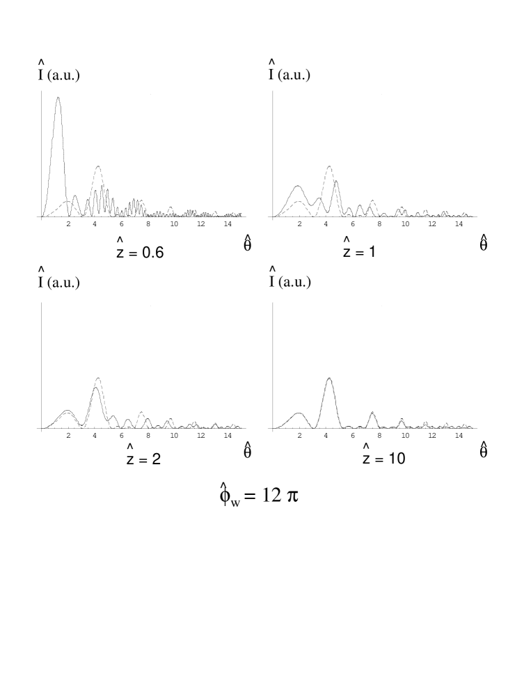
Figure 11: Evolution of the intensity profile for TUR for $\hat{\phi}_{w}=12\pi$ . These profiles are shown as a function of angles at different observation distances $\hat{z}_{o}=0.6$, $\hat{z}_{o}=1.0$, $\hat{z}_{o}=2.0$ and $\hat{z}_{o}=10.0$ (solid lines). The dashed line always refers to the far-zone intensity.

Even though it refers to a particular case where $L_{1}=L_{2}=L_{w}=L_{\mathrm{tot}}/3$, Eq. (203) still depends on the parameter $\hat{\phi}_{w}\gg 1$. Its dependence on $\hat{\phi}_{w}$ is periodic, with period $12\pi$. For the sake of exemplification, in Fig. 11 we plot the intensity profile for $\hat{\phi}_{w}=12\pi$ at different distances $\hat{z}_{o}$ and we compare these profiles with the far field asymptotic behavior. In Fig. 12 and Fig. 13 we plot, instead, the intensity profile for different values of $\hat{\phi}_{w}$ at $\hat{z}_{o}=0.6$ and in the asymptotic case for $\hat{z}_{o}\gg 1$ respectively.

Figure 12: Intensity profiles for TUR at $\hat{z}_{0}=0.6$. at different values $\hat{\phi}_{w}=(1/4)(12\pi)$, $\hat{\phi}_{w}=(1/2)(12\pi)$, $\hat{\phi}_{w}=(3/4)(12\pi)$, $\hat{\phi}_{w}=(12\pi)$.

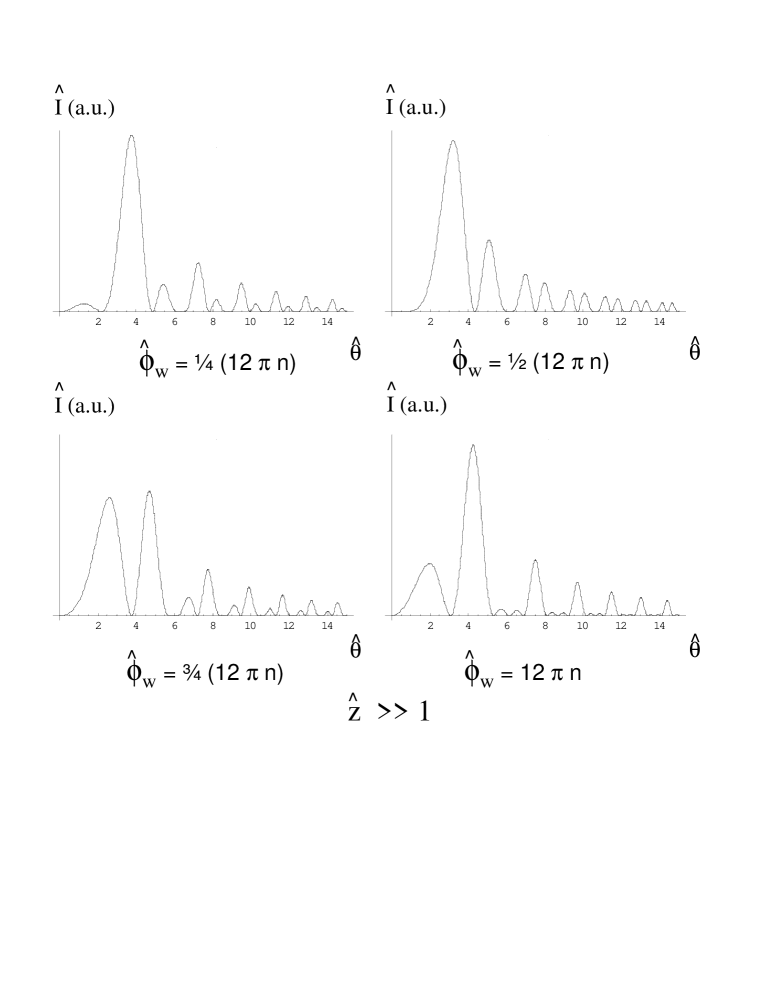
Figure 13: Intensity profiles for TUR in the asymptotic limit for $\hat{z}_{0}\gg 1$. at different values $\hat{\phi}_{w}=(1/4)(12\pi)$, $\hat{\phi}_{w}=(1/2)(12\pi)$, $\hat{\phi}_{w}=(3/4)(12\pi)$, $\hat{\phi}_{w}=(12\pi)$

7 A critical re-examination of conventional edge radiation theory

In this Section we compare our findings with treatments of edge radiation and TUR, that can be found in literature. Conventional understanding is based on the zero-length switcher approximation. This allows direct comparison of results with the contributions calculated in the previous Section 5 and Section 6. Since there is a lot of literature dealing with edge radiation and TUR we will limit ourselves to a few significative works only. In particular, we will refer to BOS4 , BOS3 , BOS7 and CHUN , even though other works report the same results. For example, the same understanding can be found in the very recent review WILL .

We found agreement with literature as concerns calculations in the far-field zone.

As we have discussed before, the far-field asymptotic is valid at observation positions $z_{o}\gg L$, independently of $\hat{\phi}=L/(\gamma^{2}\lambdabar)$. It should therefore be stressed that in the case $\hat{\phi}\gg 1$ one may be in the near zone even though the observer is located many formation lengths $\gamma^{2}\lambdabar$ from the downstream edge (for example, when $z_{o}=L$). In the far-zone case Eq. (91) gives the electric field in the far region. The correspondent directivity diagram, Eq. (100), is plotted in Fig. 4, for different values of the main parameter of the theory, $\hat{\phi}$. This result is well-known and in perfect agreement with literature. For example one may see that, aside for proportionality factors due to different choice of units, there is agreement between the radiation energy density in Eq. (97) and the photon flux per unit solid angle in Eq. (18) of BOS4 (also compare, qualitatively, Fig. 4 of that reference and our Fig. 4). Similarly, the field in Eq. (97) is in agreement with Eq. (17) of BOS3 or Eq. (31) of BOS7 (in the limit for a large observation distance) accounting for the fact that the origin of the reference system is chosen at the exit of the straight section by the author of BOS3 (also, the electron charge $e$ is negative in that reference). Note that in the far zone, the field exhibits a spherical wavefront (independently of the choice of coordinate system).

Differences between our results and results in literature arise, however, in the near zone.

7.1 Near-field edge radiation

Case for $\mathbf{\hat{\phi}\gg 1}$.

Let us pose $d=z_{o}-L/2$. In the case when $0\lesssim d\ll\gamma^{2}\lambdabar$, we have seen that the intensity profile for edge radiation reproduces better and better (as $d$ decreases) the single edge source, i.e. Eq. (123). According to our understanding then, it follows that the photon flux depends on $\gamma$, does not exhibit oscillatory dependence on the transverse position $r$, it has a characteristic scale $\gamma\lambdabar$, and depends on the frequency as $\omega^{2}(\Delta\omega/\omega)K_{1}^{2}[\omega r_{\bot}/(c\gamma)]$. In contrast to this, the flux according to Eq. (14) in BOS4 reads, in our notation (number of photons per unit surface per unit time within the bandwidth $\Delta\omega/\omega$) :

$$\frac{dF}{dS}\simeq\alpha\frac{\Delta\omega}{\omega}\frac{I_{b}}{e\pi^{2}}\frac{1}{r_{\bot}^{2}}\sin^{2}\left[\frac{\omega r_{\bot}^{2}}{4cd}\right]~{},$$ (204)

where $\alpha=e^{2}/(\hbar c)$ is the fine structure constant and $I_{b}$ is the beam current. This suggests that for $d\ll\gamma^{2}\lambda$ the photon flux does not depend on $\gamma$, exhibits oscillatory dependence on the transverse position $r_{\bot}$ on the scale $\sqrt{\lambda d}$, and depends on the frequency as $(\Delta\omega/\omega)\sin^{2}[\omega r_{\bot}^{2}/(4cd)]$. The field from which Eq. (204) is derived is given explicitly in several papers (e.g. Eq. (24) in BOS7 , Eq. (4) in BOS2 ). In our units, it reads:

$$\vec{\widetilde{E}}({z}_{o},\vec{r}_{\bot}) =-\frac{4ie}{c}\frac{\vec{{r}}_{\bot}}{{r}_{\bot}^{2}}\exp\left[-i\frac{\omega{r}_{\bot}^{2}}{4cd}\right]\sin\left[\frac{\omega{r}_{\bot}^{2}}{4cd}\right]~{}.$$ (205)

We disagree with the conclusions in Eq. (204) and Eq. (205). In particular the expression for the field in Eq. (205) is in contrast with our Eq. (116).

The region of parameters for $d\sim\gamma^{2}\lambdabar$ is not discussed in literature. As we have seen, this corresponds to a region where the near-field contribution from the downstream edge is present.

When $\gamma^{2}\lambdabar\ll d\ll L$ the contribution of the downstream edge is dominant, and the intensity distribution tends to approximate $\mathrm{const}\times\hat{\theta}^{2}/(\hat{\theta}^{2}+\hat{\phi})^{2}$, that is the single edge far field limit. This case is practically described in literature when discussing ”an electron exiting a bending magnet at the upstream end of a straight section” of infinite length (cited from BOS4 . Compare, for example with Eq. (8) in the same reference). Although this situation is per se not physical, in the sense that an infinite straight section cannot be built, it has a practical realization (for $\hat{\phi}\gg 1$) in the before-mentioned observation region $\gamma^{2}\lambdabar\ll d\ll L$.

The region of parameters for $d\sim L$ is not discussed in literature, because the near-field region is understood for $d\lesssim\gamma^{2}\lambdabar$ only. However, as we have seen, the case $d\sim L$ corresponds to a region where interference begins to become important. In our understanding, this is a transition region between the near and the far zone ($d\gg L$).

Case for $\mathbf{\hat{\phi}\ll 1}$.

In this situation we can compare results in literature with our Eq. (106). In particular, Eq. (31) of BOS7 (or, equivalently, Eq. (17) of BOS3 for the Fourier transform of the field $\vec{\bar{E}}$) is said to be applicable at for observation regions where $d\ll\gamma^{2}\lambdabar$ (using our notations) and for $L\ll\gamma^{2}\lambdabar$, i.e. when $\hat{\phi}\ll 1$. Accounting for the fact that the origin of the reference system in BOS7 is at the downstream edge of the straight section, we can write Eq. (31) of BOS7 in our dimensional units as:

$$\vec{\widetilde{E}}({z}_{o},\vec{r}_{\bot}) =\frac{2e}{c}\frac{\vec{{r}}_{\bot}}{{r}_{\bot}^{2}}\exp\left[i\frac{\omega{r}_{\bot}^{2}}{2c{z}_{o}}\right]\exp\left[i\frac{\omega{r}_{\bot}^{2}}{2c(L-2{z}_{o})}\right]$$ (207)

$$\times\left[\exp\left(-\frac{i\omega{r}_{\bot}^{2}}{2c{z}_{o}(1+2{z}_{o}/L)}\right)-\exp\left(\frac{i\omega{r}_{\bot}^{2}}{2c{z}_{o}(-1+2{z}_{o}/L)}\right)\right].$$

Thus, Eq. (31) in BOS7 appears to differ of the phase factor $\exp\{i\omega{r}_{\bot}^{2}/[2c(L-2{z}_{o})]\}$ with respect to our Eq. (106), directly calculated by propagating the field at the virtual source position. We disagree with the result in Eq. (207) (i.e. Eq. (31) in BOS7 ). The intensity pattern, however, is correct in both cases.

It is of some interest to understand the origin of the difference between our Eq. (106) and Eq. (31) in BOS7 . In this regard, in BOS7 it is reported that when $L\gg d$ (and $L\ll\gamma^{2}\lambda$) , the interference between upstream and downstream edge is negligible. In this limit, Eq. (31) in BOS7 gives back Eq. (24) in BOS7 that is Eq. (205). On the one hand Eq. (24) in BOS7 is said to be valid for an infinitely long straight section followed by a downstream edge. On the other hand, Eq. (31) in BOS7 (and thus its limiting case for $L\gg d$ as well) is reported to be valid for $d,L\ll\gamma^{2}\lambda$. Since the limiting case of Eq. (31) in BOS7 for $L\gg d$ coincides with Eq. (24) in BOS7 one concludes that an infinitely long straight section is identified de facto with the case $L\gg d$. We hold this to be a misconception, in disagreement with our understanding. The length of the straight section is naturally measured by the parameter $\hat{\phi}=L/(\gamma^{2}\lambdabar)$. Such length is independent of the position of the observer. Only when $\hat{\phi}\gg 1$ it is possible to have radiation from a single edge. In our understanding thus, the condition $L\gg d$ is still necessary, but not sufficient to have single-edge radiation. Describing the situation for $\hat{\phi}\ll 1$ we have seen from Eq. (106) that the total field is always given as the result of the interference of the two virtual sources located at the straight section edges and one never has radiation from single edge. In contrast to this radiation from a single edge (in Eq. (24) of BOS7 ) is explicitly reported to hold for $L\ll\gamma^{2}\lambda$ in the limit for $L\gg d$.

We conclude that the origin of the difference between our results and those in literature may be ascribed to a different understanding of the parameters of the theory. While we hold $\hat{\phi}$ to be the main parameter of our treatment, result in literature seem to neglect its existence. By doing this, conventional treatments neglect the fact that $d$ and $L$ should always be compared with the third main length scale of the problem, that is $\gamma^{2}\lambdabar$.

7.2 Transition Undulator Radiation

As we have seen, TUR can be addressed as a more complicated edge-radiation setup. In this case we have contributions from three parts, two straight lines and the undulator. As we have seen, the undulator contribution is similar to a straight line contribution, the only difference being a different average longitudinal velocity of the electron. Then, the far-zone region can be identified by distances $z_{o}\gg L_{tot}$. In the far zone, well-accepted expressions for the TUR emission are reported in literature KIM1 , KINC , CAST , that are equivalent to the following equation for the radiation energy density as a function of angle and frequency:

$$\frac{dW}{d\omega d\Omega} = \frac{e^{2}}{\pi^{2}c}\left[\frac{2\gamma^{2}\theta K^{2}}{(1+K^{2}/2+\gamma^{2}\theta^{2})(1+\gamma^{2}\theta^{2})}\right]^{2}\sin^{2}\left[\frac{\pi L_{w}}{2\gamma^{2}\lambda}\left(1+\frac{K^{2}}{2}+\gamma^{2}\theta^{2}\right)\right].$$ (208)

We disagree with this expression. In our understanding, there cannot be any range of parameters in the setup in Fig. 10 where Eq. (LABEL:wron3) is valid.

In order to prove this it is sufficient to compare Eq. (LABEL:wron3) with Eq. (168), that is equivalent to Eq. (20) of reference BOS4 . In particular, since Eq. (LABEL:wron3) does not depend on the straight section lengths $L_{1}$ or $L_{2}$, we conclude that the only regions where such comparison makes sense can be for $L_{1}=L_{2}=0$, or $L_{1}=L_{2}=L_{w}$ .

When $L_{1}=L_{2}=0$ Eq. (168) reduces to:

$$\frac{dW}{d\omega d\Omega}=\frac{e^{2}}{\pi^{2}c}\left[\frac{2\gamma^{2}\theta}{1+K^{2}/2+\gamma^{2}\theta^{2}}\right]^{2}\sin^{2}\left[\frac{\pi L_{w}}{2\gamma^{2}\lambda}\left({1}+\frac{K^{2}}{2}+\gamma^{2}\theta^{2}\right)\right]~{},$$ (210)

that is obviously different from Eq. (LABEL:wron3.)

When $L_{1}=L_{2}=L_{w}$ Eq. (168) becomes:

$$\frac{dW}{d\omega d\Omega} = \frac{e^{2}}{\pi^{2}c}\left[\frac{2\gamma^{2}\theta K^{2}}{(1+K^{2}/2+\gamma^{2}\theta^{2})\left(1+\gamma^{2}\theta^{2}\right)}\right]^{2}$$ (211)

$$\times \Bigg{|}\frac{1}{2}~{}{\sin\left[\frac{\pi L_{w}}{2\gamma^{2}\lambda}\left({1}+\frac{K^{2}}{2}+\gamma^{2}\theta^{2}\right)\right]}$$ (213)

$$-\frac{(1+K^{2}/2+\gamma^{2}\theta^{2})}{K^{2}}\sin\left[\frac{\omega L_{w}}{4c\gamma^{2}}\left(3+\frac{K^{2}}{2}+3\gamma^{2}\theta^{2}\right)\right]\Bigg{|}^{2}~{},$$

that is also different from Eq. (LABEL:wron3). We conclude that Eq. (LABEL:wron3) has no physical meaning.

Finally, we put attention on the fact that there is a general need, in the FEL community, to extend the current theory of TUR to cover the near zone. Some attempt in this direction has been reported in ADA1 . The author of ADA1 discusses a possible use of coherent TUR to produce visible-to-infrared light synchronized with X-rays from an X-ray free-electron laser. For simplicity we will ignore the delicate issue of technical realization of the scheme proposed in ADA1 for the LCLS facility, and we will restrict our discussion of a issue pertaining fundamental questions of electrodynamics.

In our view, the extension of the theory of TUR in Appendix A of ADA1 to the near zone also includes some misconceptions. The treatment begins with Eq. (A1), that is an expression for the vector potential $\vec{A}$ at a given observation position and at a given frequency of interest. We report this expression here, for the readers’ commodity:

$$\vec{A}(\omega)\sim\int_{-T/2}^{T/2}\exp\left[i\omega\left(t+R(t)/c\right)\right]\frac{d}{dt}\left[\frac{\vec{n}\times\left(\vec{n}\times\vec{\beta}\right)}{1-\vec{\beta}\cdot\vec{n}}\right]~{}.$$ (214)

Here $T=L/c$ is the time that a photon takes to travel the undulator length, $R(t)$ is the distance from the electron position at retarded time $t$ to the observer, the unit vector $\vec{n}$ is the direction from the retarded position of the electron to the observer and $\vec{\beta}(t)$ is the electron velocity in units of the speed of light. Eq. (214) is a modification of the well-known Eq. (14.62) of JACK . In fact, integration limits in Eq. (214) have been changed from $\pm\infty$ to $\pm T/2$ ”under the assumption that the electrons go on straight paths before and after the undulator” (cited from ADA1 ). As a first remark, as discussed above, the previous assumption is not justified in our view, as it does not make sense to discuss generically about infinite straight lines preceding and following the undulator. However, we believe that there is another problem with the use made of Eq. (214). The author of ADA1 starts with Eq. (214) and modifies it accounting for the fact that, in the near zone, $\vec{n}$ is not constant. The problem with this is that the derivation of Eq. (214) relies a priori on the assumption that $\vec{n}=\mathrm{const}$. In particular, the classical result

$${\vec{n}\times[(\vec{n}-\vec{\beta})\times{\dot{\vec{\beta}}}]\over{(1-\vec{n}\cdot\vec{\beta})\left|\vec{r}_{o}-\vec{r^{\prime}}(t)\right|}}={1\over{r_{o}}}{d\over{dt}}\left[{\vec{n}\times(\vec{n}\times{\vec{\beta}})\over{1-\vec{n}\cdot\vec{\beta}}}\right]~{},$$ (215)

is used, where $r_{o}=|\vec{r}_{o}|$ is the distance of the observer from the origin of the coordinate system. Eq. (215) assumes $\vec{n}=\mathrm{const}$.

Our conclusion is that Eq. (214) cannot be manipulated assuming that $\vec{n}$ is not constant, as has been done in ADA1 . When $\vec{n}$ is not constant, as in this case, Eq. (215) should be modified to the expression presented before in Eq. (65) that may be found in the interesting but perhaps little-known reference LUCC , dating back more than twenty years.

However, in this paper we have seen that it is possible to develop a more convenient theory of near-field Synchrotron Radiation Theory (including the case of TUR) in the space-frequency domain, where Fourier Optics techniques can be taken advantage of.

8 Conclusions

In this paper we presented a general connection between Fourier Optics and classical relativistic electrodynamics. Consistent use of such connection resulted in the formulation of a modern theory of Synchrotron Radiation in terms of laser-beam optics.

In particular, we developed a theory of near-field SR in the space-frequency domain based of Fourier Optics techniques. These techniques can be taken advantage of without limitations for SR setups, because the paraxial approximation can always be applied in the case of electrons in ultra-relativistic motion. We restricted ourselves to the analysis of single-particle radiation. As we demonstrated in Section 2, and discussed in Section 3 the use of paraxial approximation allows reconstruction of the field in the near-zone from the knowledge of far-field data only. The solvability of the inverse problem for the field starting from far-field data allows characterization of any synchrotron radiation setup by means of virtual sources. In cases of interest these sources exhibit a plane wavefront, and can be pictured as waists of laser-like beams. These laser-like beams help developing our theory in close relation with laser-beam optics. In particular, usual Fourier Optics can be used to describe the field at any distance, thus providing a tool for designing and analyzing SR setups.

We gave several examples of applications of our theory in Section 4, Section 5 and Section 6. These examples provide both physical insight and understanding of several non-intuitive phenomena. In Section 4 we treated the case of undulator radiation. In the case of perfect resonance we found an analytic expression for the virtual source and we propagated such expression both in the near and in the far zone. The applications in the following Section 5 and Section 6 actually constitute the first comprehensive theory of edge radiation and transition undulator radiation.

In Section 5 we dealt with the fundamental case of an electron moving on a straight section. Such kind of system can be considered, in all generality, as a fundamental building block for a number of more complicated setups. We demonstrated that two equivalent pictures in terms of laser-like sources can be presented. The first takes advantage of a single virtual source in the middle of the straight section. The second relies on two virtual sources at the edges. The virtual sources at the edges can always be described analytically, independently of the region of parameters considered. The main parameter of the theory is identified to be the ratio between the straight section length $L$ and $\gamma^{2}\lambdabar$. When this ratio is small the single-source picture is found to be natural, and two asymptotic regions of observation are found, the near and the far zone. When the ratio is large, the two-source picture is more natural and one is left with four asymptotic regions of observation: far zone for two interfering sources, near zone for two interfering sources, far zone for a single edge and near zone for a single edge. Results in Section 5 can be directly used to describe an edge-radiation setup in the case upstream and downstream bends can be considered to have zero length. These bends act like switchers, switching the radiation harmonic (and the beam current harmonic) on and off. Thus, our results for the straight section can be applied to any situation with zero-length switchers. Our expressions are of importance also in the case when switchers cannot be considered having zero-length. In fact in general, as said before, straight sections can be considered as basic building blocks for any magnetic setup.

To demonstrate this last point, in Section 6 we used results of Section 5 as building blocks for describing the case of TUR in the zero-length switcher approximation. In particular, we dealt with a setup composed by an undulator preceded and followed by two straight sections. In the zero-length switchers approximation, such setup describes TUR emission. Although more sophisticated with respect to the straight-section motion, the example in Section 6 does not present any conceptual difficulty in addition to those encountered in the treatment of the straight-section motion.

Finally, in Section 7, we compared our findings with current understanding of edge radiation and TUR. We found that several misconceptions exist in the conventional understanding of edge radiation in the near zone, as well as in the treatment of TUR. We extensively discussed these misconceptions and proposed our understanding of the correct description of these phenomena.

We find it interesting to remark that, although classical relativistic electrodynamics is a relatively old branch of physics, there are many novel and valuable results pertaining this field that have been obtained only recently. Undoubtedly, many more will follow. These recent developments illustrate a recurring fact in the history of Physics. Namely, subjects appearing well-understood, and perhaps even a little old-fashioned may still have surprises in store for us.

9 Acknowledgements

The authors are grateful to Martin Dohlus, Hermann Franz, Petr Ilinski and Helmut Mais (DESY) for many useful discussions and to Massimo Altarelli, Edgar Weckert and Jochen Schneider (DESY) for their interest in this work.

References

- [1] G. Geloni, E. Saldin, E. Schneidmiller and M. Yurkov, ”Paraxial Green’s functions in SR theory”, DESY 05-032, ISSN 0418-9833 (2005)
- [2] G. Geloni, E. Saldin, E. Schneidmiller and M. Yurkov, ”Understanding transverse coherence properties of X-ray beams in third generation SR source”, DESY 05-109, ISSN 0418-9833 (2005)
- [3] G. Geloni, E. Saldin, E. Schneidmiller and M. Yurkov, ”Statistical Optics approach to the design of beamlines for Synchotron Radiation”, DESY 06-037, ISSN 0418-9833 (2006)
- [4] J. W. Goodman, ”Introduction to Fourier Optics”, Mc Graw-Hill Book Company(1968)
- [5] ZEMAX code, at http://www.zemax.com/
- [6] R.A. Bosch et al. Rev. Sci. Instrum. 67, 3346 (1995)
- [7] R.A. Bosch and O.V. Chubar, ”Long wavelength edge radiation in an electron storage ring”, Proc. SRI’97, tenth US National Conference, AIP Conf. Proc. 417, edited by E. Fontes (AIP, Woodbury, NY), pp. 35-41 (1997)
- [8] R.A. Bosch, Il Nuovo Cimento, 20, 4 p. 483 (1998)
- [9] R.A. Bosch, Nucl. Instr. Meth. Phys. Res. A, 431 (1999) 320
- [10] P. Roy, J-B. Brubach et al., Nucl. Instr. Meth. Phys. Res. A, 426 (2001)
- [11] R.A. Bosch, Nucl. Instr. Meth. Phys. Res. A, 482, 789 (2002)
- [12] R.A. Bosch, Phys. Rev. ST AB 5, 020701 (2002)
- [13] G. P. Williams, Rep. Prog. Phys. 69 (2006), 301
- [14] K.-J. Kim, Phys. Rev. Lett. 76, 8 (1996)
- [15] B.M. Kincaid, Il Nuovo Cimento Soc. Ital. Fis, 20D, 495 (1998) and LBL-38245 (1996)
- [16] M. Castellano, Nucl. Instr and Meth. in Phys. Res. A 391 (1997) 375
- [17] R.A. Bosch, Nucl. Instr. Meth. Phys. Res. A, 386 (1997) 525
- [18] P. Roy et al. Phys. Rev. Lett. 84, 3 (2000)
- [19] S. Reiche and Z. Huang, in Proceedings of the 2004 FEL Conference, R. Bakker et al. Editors, Trieste, pp. 193-195 (2004)
- [20] B. Adams, Rev. Sci. Instrum. 76, 2 (2005)
- [21] J. Jackson, ”Classical Electrodynamics”, 3rd ed., Wiley, New York (1999)
- [22] O. Chubar and P. Elleaume, in Proc. of the 6th European Particle Accelerator Confernce EPAC-98, 1177-1179 (1998)
- [23] Y. Hirai, A. Luccio and Li-hua Yu, J. Appl. Phys. 55(1), 25 (1984)
- [24] G. Geloni, E. Saldin, E. Schneidmiller and M. Yurkov, ”Exact solution for the Second Harmonic Generation in XFELs”, DESY 05-137, ISSN 0418-9833 (2005), submitted to Optics Communications
- [25] J. Bahrdt, in Proceedings of the 2005 FEL Conference, R. Reitmeyer Editor, Stanford, pp. 694-701 (2005)