Charge-Resonance Effect on Harmonic Generation by Symmetric Diatomic Molecular Ions in Intense Laser Fields

Abstract

In present paper we develop an analytic theory for the harmonic generation of symmetric diatomic molecular ions beyond two-level model, emphasizing the influence of charge-resonance (CR) states those are strongly coupled to electromagnetic fields for large internuclear distance. With taking into account the continuum states that is ignored in the two-level model and become important for intense laser case, our model is capable to produce spectrum for the whole range of harmonic orders consisting of a molecular plateau due to the CR transition and an atomic-like plateau for a long-wavelength excitation, and in good agreement with numerical results from directly solution of the Schrödinger equation. Our theory also identifies the crucial role of the CR states in the fine structure of harmonic spectrum and shows that the harmonic generation in molecular system can be effectively controlled by adjusting the internuclear distance.

I Introduction

In recent years, high order harmonic generation (HOHG) from atom and molecule has been the subject of numerous experimental and theoretical studies, mainly because the emission of high-order harmonics is a promising method to produce coherent x rays and attosecond pulses, and an effective ways to study the internal construction of atom or molecule1 ; 2 ; 3 ; 4 ; 5 ; 6 ; 7 ; 8 ; 9 ; 10 ; 11 ; 12 ; 13 ; 14 ; 15 ; 16 ; 17 ; 18 ; 19 ; 20 ; 21 ; 22 .

Compared to atom case, the HOHG spectrum of molecule systems demonstrates novel properties, e.g., peak splitting and sideband peaks, Rabi or Mollow triplets effect, and combination of the atomic-like and molecular-like plateau, molecular alignment effect, and two-center interference, to name only a few23 ; 24 ; 25 ; 26 . Symmetric molecular system such as $H_{2}^{+}$ have pairs of electronic states known as the charge-resonance (CR) states, (i.e.,$1\sigma_{g}$,$1\sigma_{\mu}$.) It is known that the CR states are strongly coupled to electromagnetic fields at large internuclear separation $R$. Bandrauk and co-worker first pointed out the importance of these CR states as sources of highly nonlinear laser-induced effects in molecules23 . Ivanov, Corkum examined the possibility of using the CR states to produce and coherently control HOHG24 . Zuo, Chelkowski, and Bandrauk have showed that symmetric molecular ions in general produce more efficient harmonic generation than atoms, especially at large $R$, due to these CR states25 ; 26 . However, in the all above discussions, the theoretical analysis is based on a two-level model where the continuum (ionization) states are ignored completely. Since the ground-continuum coupling and ionization become important for the strong laser fields of $10^{14}W/cm^{2}$ and above, a fully understanding of the whole structure of HOHG and the effect of CR states in molecule systems requires to extend to consider the continuum states and ionization process.

In present paper we develop an analytic theory on the harmonic generation of symmetric diatomic molecular ions beyond the two-level model. Our model is capable to produce harmonic structure for the whole range of harmonic order, including the molecular plateau due to CR transition and the atomic-like plateau for a long-wavelength excitation, and agrees well with the numerical results from directly solving the Schrödinger equation. Our theory identifies the role of the CR states in the fine structure of harmonic spectrum and shows that the harmonic generation in molecular system can be effectively controlled through CR states by adjusting the internuclear distance.

Our paper is organized as follows. In Sec.II we present our analytical theory. Our analysis is divided into two cases: near-resonance region of intermediate internuclear distance and the strong-coupling region of large internuclear distance. We will derive the time-dependent amplitudes of the ground, excited and continuum states, then calculate dipolar moments and their Fourier transformation. The analytic expressions of the amplitudes of HOHG for the whole range of harmonic order is given in this section. Sec.III presents our numerical results. Our theory is applied to 1D symmetric diatomic molecule model, making analysis on the structure of HOHG and compare with the results from directly solving Schrödinger equation. Sec.V is our conclusion.

II Analytic theory

We consider a diatomic molecule ion in single-electron approximation under the influence of a linear polarized laser field $\mathbf{A}(t)=(E\cos({\omega}t),0,0)$, where $E{\omega}$ is the absolute amplitude of the external electric field and ${\omega}$ is the frequency of the external field. The Hamiltonian of the model molecule studied here is

$$\begin{split}H(t)=(\mathbf{p}-\mathbf{A}(t))^{2}/2+V(\mathbf{r}),\end{split}$$

where $\mathbf{p}$ is the canonical momentum and $V(\mathbf{r})$ is the binding potential.

Under strong-field conditions 27 ; 28 , it is reasonable to assume that, (a) Except the ground state $|0\rangle$ and the first excited state$|1\rangle$, the contribution from other bound states can be neglected;(b) The depletion of the ground state and the first excited state is small;(c) In the continuum, the electron can be treated as a free particle moving in the electric field without considering Coulomb potential. Then, the time-dependent wave functions can be expanded as

$$|\psi(t)\rangle=e^{-iE_{0}t}[a(t)|0\rangle+b(t)|1\rangle+\int d\mathbf{p}c_{\mathbf{p}}(t)|\mathbf{p}\rangle],$$ (1)

where $-E_{0}$ is the ionization potential of the ground state, $a(t)$ is the ground-state amplitude, $b(t)$ is the first excited state amplitude and $c_{\mathbf{p}}(t)$ are the amplitudes of the corresponding continuum states. While the ionization is weak, by neglecting the depletion of the ground and the first excited state and setting $|a(t)|^{2}+|b(t)|^{2}=1$, the formulation of $a(t)$ and $b(t)$ can be obtained by a two-level approximation. We have factor out here free oscillations of the ground-state amplitude by the bare frequency $-E_{0}$. The Schr$\ddot{o}$dinger equation for $c_{\mathbf{p}}(t)$ reads as

$$\dot{c}_{\mathbf{p}}(t)=i\mathbf{A}(t)\mathbf{p}[a(t)\langle\mathbf{p}|0\rangle+b(t)\langle\mathbf{p}|1\rangle]+[(\mathbf{p}-\mathbf{A}(t))^{2}/2-E_{0}]c_{\mathbf{p}}(t).$$ (2)

(2) can be solved exactly and $c_{\mathbf{p}}(t)$ can be written in the closed form

$$\begin{split}c_{\mathbf{p}}(t)=i\int_{0}^{t}dt^{\prime}\mathbf{A}(t^{\prime})\mathbf{p}[a(t^{\prime})\langle\mathbf{p}|0\rangle+b(t^{\prime})\langle\mathbf{p}|1\rangle]\\ \times e^{-i\int_{t^{\prime}}^{t}[(\mathbf{p}-\mathbf{A}(t^{\prime\prime}))^{2}/2-E_{0}]dt^{\prime\prime}}.\end{split}$$ (3)

Using Eq. (1) and (3), the mechanical momentum $\mathbf{p}-\mathbf{A}(t)$ component of the time-dependent dipole moment is

$${\bf D}(t)=\langle\psi(t)|{\mathbf{p}}-\mathbf{A}(t)|\psi(t)\rangle.$$ (4)

Neglecting the term $\langle\psi(t)|\mathbf{A}(t)|\psi(t)\rangle$=$\mathbf{A}(t)$, which only includes the fundamental frequency ${\omega}$, and the contribution from C-C part and considering only the transitions back to the ground state and the first excited state, we obtain ${\bf D}(t)=D_{0}(t)+D_{1}(t)$,where

$$\begin{split}D_{0}(t)=i\int d\mathbf{p}\int_{0}^{t}dt^{\prime}a^{*}(t)\langle 0|{\mathbf{p}}|\mathbf{p}\rangle\mathbf{A}(t^{\prime})\cdot\mathbf{p}\big{[}a(t^{\prime})\langle\mathbf{p}|0\rangle\\ +b(t^{\prime})\langle\mathbf{p}|1\rangle\big{]}\times e^{-iS(\mathbf{p},t,t^{\prime})},\end{split}$$ (5)

$$\begin{split}D_{1}(t)=i\int d\mathbf{p}\int_{0}^{t}dt^{\prime}b^{*}(t)\langle 1|{\mathbf{p}}|\mathbf{p}\rangle\mathbf{A}(t^{\prime})\cdot\mathbf{p}\big{[}a(t^{\prime})\langle\mathbf{p}|0\rangle\\ +b(t^{\prime})\langle\mathbf{p}|1\rangle\big{]}\times e^{-iS(\mathbf{p},t,t^{\prime})},\end{split}$$ (6)

where $S(\mathbf{p},t,t^{\prime})=\int_{t^{\prime}}^{t}\left[(\mathbf{p}-\mathbf{A}(t^{\prime\prime}))^{2}/2-E_{0}\right]dt^{\prime\prime}$. $D_{0}(t)$ denotes the transition back to the ground state, and $D_{1}(t)$ denotes the transition back to the first excited state. Each of $D_{0}(t)$ and $D_{1}(t)$ includes two different terms, which denote two different moments, respectively. For $D_{0}(t)$, they are $|0\rangle\rightarrow|\mathbf{p}\rangle\rightarrow|0\rangle$ (denoted by $D_{0}^{0}(t)$) and $|1\rangle\rightarrow|\mathbf{p}\rangle\rightarrow|0\rangle$ (denoted by $D_{0}^{1}(t)$), which denote the transition from the ground state to the continuum state, then back to the ground state($D_{0}^{0}(t)$), or from the first excited state to the continuum state, then back to the ground state($D_{0}^{1}(t)$); for $D_{1}(t)$,they are $|0\rangle\rightarrow|\mathbf{p}\rangle\rightarrow|1\rangle$ (denoted by $D_{1}^{0}(t)$) and $|1\rangle\rightarrow|\mathbf{p}\rangle\rightarrow|1\rangle$ (denoted by $D_{1}^{1}(t)$), which denote the transition from the ground state to the continuum state, then back to first excited state($D_{1}^{0}(t)$), or from the first excited state to the continuum state, then back to first excited state($D_{1}^{1}(t)$). We should discuss these moments at intermediate $R$ and large $R$, respectively.

II.1 Intermediate $R$ with $(E_{1}-E_{0})/{\omega}\simeq 1$

For a two-level system, the time-dependent wave function can be written as $|\psi(t)\rangle$=$a(t)|0\rangle+b(t)|1\rangle$, where $|0\rangle$ and $|1\rangle$ are the ground-state and the first excited state of the unperturbed Hamiltonian $H_{0}={{\mathbf{p}}}^{2}+V({\vec{r}})$ with $H_{0}|0\rangle=E_{0}|0\rangle$ and $H_{0}|1\rangle=E_{1}|1\rangle$. While $(E_{1}-E_{0})/{\omega}\simeq 1$, in the rotating-wave approximation, the solution for $a(t)$ and $b(t)$ can be written as

$$\left\{\begin{array}[]{ll}a(t)=e^{-iE_{0}t-i\int_{0}^{t}[\mathbf{A}^{2}(t^{\prime})/2]dt^{\prime}}(a_{1}e^{iQt/2}+a_{2}e^{-iQt/2})e^{-i\xi t/2},\\ b(t)=e^{-iE_{1}t-i\int_{0}^{t}[\mathbf{A}^{2}(t^{\prime})/2]dt^{\prime}}(b_{1}e^{iQt/2}+b_{2}e^{-iQt/2})e^{i\xi t/2},\end{array}\right.$$

and by the Bessel function formula29 ,we obtain finally

$$\left\{\begin{array}[]{ll}a(t)=\sum_{n=-\infty}^{n=+\infty}J_{n}(E^{2}/8{\omega})(a_{1}e^{-iA_{1}t}+a_{2}e^{-iA_{2}t})\\ b(t)=\sum_{n=-\infty}^{n=+\infty}J_{n}(E^{2}/8{\omega})(b_{1}e^{-iB_{1}t}+b_{2}e^{-iB_{2}t}),\end{array}\right.$$ (10)

where $E{\omega}$ is the absolute amplitude of the external electric field and$A_{1}=E^{2}/4+2n{\omega}-Q/2+\xi/2,$ $A_{2}=E^{2}/4+2n{\omega}+Q/2+\xi/2,$ $B_{1}=E_{1}+E^{2}/4+2n{\omega}-Q/2-\xi/2-E_{0},$ $B_{2}=E_{1}+E^{2}/4+2n{\omega}+Q/2-\xi/2-E_{0},$ where $\xi$=$E_{1}-E_{0}-{\omega}$; $Q$=$\sqrt{|Q_{R}|^{2}+\xi^{2}}$, $Q_{R}$=$ED$, $D$=$\langle 0|{\mathbf{p}}|1\rangle$ is the matrix element of the electric dipole moment, and $a_{1},a_{2},b_{1}$ and $b_{2}$ are constants of integration which are determined from the initial conditions $|\psi(0)\rangle$=$a(0)|0\rangle+b(0)|1\rangle$:

$$\left\{\begin{array}[]{ll}a_{1}=[(Q+\xi)a(0)+Q_{R}b(0)]/(2Q)\\ a_{2}=[(Q-\xi)a(0)-Q_{R}b(0)]/(2Q)\\ b_{1}=[(Q-\xi)b(0)+Q_{R}^{*}a(0)]/(2Q)\\ b_{2}=[(Q+\xi)b(0)-Q_{R}^{*}a(0)]/(2Q),\end{array}\right.$$ (15)

where $Q_{R}^{*}$ is the conjugated element of $Q_{R}$. For the convenience of latter calculation, we have multiplied $a(t)$ and $b(t)$ by a phasic factor $e^{iE_{0}t}$. Substituting (8) into (5) and (6), then it follows:

II.1.1 $|0\rangle\rightarrow|\mathbf{p}\rangle\rightarrow|0\rangle$

For $D_{0}(t)$, above all we consider the moment$|0\rangle\rightarrow|\mathbf{p}\rangle\rightarrow|0\rangle$ , i.e.,

$$\begin{split}D_{0}^{0}(t)=i\int d\mathbf{p}\int_{0}^{t}dt^{\prime}a^{*}(t)\langle 0|{\mathbf{p}}|\mathbf{p}\rangle{\mathbf{A}(t^{\prime})\cdot\mathbf{p}a(t^{\prime})\langle\mathbf{p}|0\rangle e^{-iS(\mathbf{p},t,t^{\prime})}},\end{split}$$ (16)

For $e^{-iS(\mathbf{p},t,t^{\prime})}$, by the formula $e^{-i\gamma sin(2{\omega}t)+i\kappa Esin({\omega}t)}=\sum_{n=-\infty}^{n=+\infty}J_{n}(-\kappa,\gamma)e^{-in{\omega}t}$, we can obtain

$$\begin{split}e^{-iS(\mathbf{p},t,t^{\prime})}=&e^{-i(E^{2}/4+\mathbf{p}^{2}/2-E_{0})(t-t^{\prime})}\sum_{n,m=-\infty}^{n,m=+\infty},\\ &J_{n}(\frac{-p_{x}E}{{\omega}},\frac{E^{2}}{8{\omega}})J_{m}(\frac{p_{x}E}{{\omega}},\frac{-E^{2}}{8{\omega}})e^{-in{\omega}t}e^{-im{\omega}t^{\prime}},\end{split}$$

substituting it into (9), and integrating over $t^{\prime}$, we obtain

$$\begin{split}&D_{0}^{0}(t)=i\int d\mathbf{p}\frac{E}{2}\langle 0|\mathbf{p}\rangle\mathbf{p}(\mathbf{p}_{x})\langle\mathbf{p}|0\rangle\\ &\sum_{n,m,n_{1},m_{1}=-\infty}^{n,m,n_{1},m_{1}=+\infty}\bigg{\{}\frac{a_{1}^{*}a_{1}e^{-i(C_{1}+A_{1}^{\prime}+D_{1}-A_{1})t}}{-i(C_{1}+A_{1}^{\prime})}\\ &+\frac{a_{1}^{*}a_{2}e^{-i(C_{1}+A_{2}^{\prime}+D_{1}-A_{1})t}}{-i(C_{1}+A_{2}^{\prime})}+\frac{a_{1}^{*}a_{1}e^{-i(C_{2}+A_{1}^{\prime}+D_{1}-A_{1})t}}{-i(C_{2}+A_{1}^{\prime})}\\ &+\frac{a_{1}^{*}a_{2}e^{-i(C_{2}+A_{2}^{\prime}+D_{1}-A_{1})t}}{-i(C_{2}+A_{2}^{\prime})}+\frac{a_{2}^{*}a_{1}e^{-i(C_{1}+A_{1}^{\prime}+D_{1}-A_{2})t}}{-i(C_{1}+A_{1}^{\prime})}\\ &+\frac{a_{2}^{*}a_{2}e^{-i(C_{1}+A_{2}^{\prime}+D_{1}-A_{2})t}}{-i(C_{1}+A_{2}^{\prime})}+\frac{a_{2}^{*}a_{1}e^{-i(C_{2}+A_{1}^{\prime}+D_{1}-A_{2})t}}{-i(C_{2}+A_{1}^{\prime})}\\ &+\frac{a_{2}^{*}a_{2}e^{-i(C_{2}+A_{2}^{\prime}+D_{1}-A_{2})t}}{-i(C_{2}+A_{2}^{\prime})}\bigg{\}}J_{n}J_{m}J_{n_{1}}J_{m_{1}},\end{split}$$

where $J_{m}$=$J_{m}(\frac{p_{x}E}{{\omega}},\frac{-E^{2}}{8{\omega}})$, $J_{m_{1}}$=$J_{m_{1}}(\frac{-p_{x}E}{{\omega}},\frac{E^{2}}{8{\omega}})$, $J_{n}$=$J_{n}(\frac{E^{2}}{8{\omega}})$, $J_{n_{1}}$=$J_{n_{1}}(\frac{E^{2}}{8{\omega}})$,and $A_{1}=E^{2}/4+2n_{1}{\omega}-Q/2+\xi/2,$ $A_{2}=E^{2}/4+2n_{1}{\omega}+Q/2+\xi/2,$ $C_{1}=m{\omega}-\mathbf{p}^{2}/2-E^{2}/4+E_{0}-{\omega},$ $C_{2}=m{\omega}-\mathbf{p}^{2}/2-E^{2}/4+E_{0}+{\omega},$ $A_{1}^{\prime}=E^{2}/4+2n{\omega}-Q/2+\xi/2,$ $A_{2}^{\prime}=E^{2}/4+2n{\omega}+Q/2+\xi/2,$$D_{1}=\mathbf{p}^{2}/2+E^{2}/4-E_{0}+m_{1}{\omega}.$

The Fourier component of $D_{0}^{0}(t)$ reads as

$$\begin{split}&P_{0}^{0}({\omega}^{\prime})=-i\int d\mathbf{p}E\pi\langle 0|\mathbf{p}\rangle\mathbf{p}p_{x}\langle\mathbf{p}|0\rangle\sum_{n,m,n_{1},m_{1}=-\infty}^{n,m,n_{1},m_{1}=+\infty}J_{n}J_{m}\\ &\Bigg{\{}\frac{a_{1}^{*}a_{1}\delta\left[(m+m_{1}-1+2(n-n_{1})){\omega}-{\omega}^{\prime}\right]}{(C_{1}+A_{1}^{\prime})}\\ &+\frac{a_{2}^{*}a_{2}\delta\left[(m+m_{1}-1+2(n-n_{1})){\omega}-{\omega}^{\prime}\right]}{(C_{1}+A_{2}^{\prime})}\\ &+\frac{a_{1}^{*}a_{1}\delta\left[(m+m_{1}+1+2(n-n_{1})){\omega}-{\omega}^{\prime}\right]}{(C_{2}+A_{1}^{\prime})}\\ &+\frac{a_{2}^{*}a_{2}\delta\left[(m+m_{1}+1+2(n-n_{1})){\omega}-{\omega}^{\prime}\right]}{(C_{2}+A_{2}^{\prime})}\\ &+\frac{a_{1}^{*}a_{2}\delta\left[(m+m_{1}-1+2n-2n_{1}){\omega}+Q-{\omega}^{\prime}\right]}{(C_{1}+A_{2}^{\prime})}\\ &+\frac{a_{1}^{*}a_{2}\delta\left[(m+m_{1}+1+2n-2n_{1}){\omega}+Q-{\omega}^{\prime}\right]}{(C_{2}+A_{2}^{\prime})}\\ &+\frac{a_{2}^{*}a_{1}\delta\left[(m+m_{1}-1+2n-2n_{1}){\omega}-Q-{\omega}^{\prime}\right]}{(C_{1}+A_{1}^{\prime})}\\ &+\frac{a_{2}^{*}a_{1}\delta\left[(m+m_{1}+1+2n-2n_{1}){\omega}-Q-{\omega}^{\prime}\right]}{(C_{2}+A_{1}^{\prime})}\Bigg{\}}J_{n_{1}}J_{m_{1}}\end{split}$$ (17)

For(10),the parity of $\langle 0|\mathbf{p}\rangle\mathbf{p}p_{x}\langle\mathbf{p}|0\rangle$ for the integral over $\mathbf{p}$ is even, according to the property of Bessel function, only when $m+m_{1}$ is even, the value of Eq. (10) for the integral over $\mathbf{p}$ is not zero. Fourier components on the right-hand side of (10) can be divided into two parts, odd Fourier components of $(m+m_{1}+2n-2n_{1}\pm 1){\omega}$, and no-integer Fourier components of $(m+m_{1}+2n-2n_{1}\pm 1){\omega}\pm Q$ .It also can be seen from (10), the Rabi oscillation of the ground and first excited state should not contribute to the parity of integer harmonic, but induces the symmetrical splitting of odd harmonic. The splitting separations around each odd harmonic all take the same value $Q$. If $Q/{\omega}$ is integer of odd number, then the odd harmonic sidebands should coincide at the even harmonic ($2n{\omega}$) position, thus giving rise to radiation of even harmonics.

II.1.2 $|1\rangle\rightarrow|\mathbf{p}\rangle\rightarrow|0\rangle$

For $|1\rangle\rightarrow|\mathbf{p}\rangle\rightarrow|0\rangle$, i.e.,

$$D_{0}^{1}(t)=i\int d\mathbf{p}\int_{0}^{t}dt^{\prime}a^{*}(t)\langle 0|{\mathbf{p}}|\mathbf{p}\rangle{\mathbf{A}(t^{\prime})\cdot\mathbf{p}b(t^{\prime})\langle\mathbf{p}|1\rangle e^{-is(\mathbf{p},t,t^{\prime})}}.$$

Analogous to $|0\rangle\rightarrow|\mathbf{p}\rangle\rightarrow|0\rangle$, the Fourier component of $D_{0}^{1}(t)$ reads as

$$\begin{split}&P_{0}^{1}({\omega}^{\prime})=-i\int d\mathbf{p}E\pi\langle 0|\mathbf{p}\rangle\mathbf{p}p_{x}\langle\mathbf{p}|1\rangle\sum_{n,m,n_{1},m_{1}=-\infty}^{n,m,n_{1},m_{1}=+\infty}J_{n}J_{m}\\ &\Bigg{\{}\frac{a_{1}^{*}b_{1}\delta\left[(m+m_{1}+2n-2n_{1}){\omega}-{\omega}^{\prime}\right]}{(C_{1}+B_{1}^{\prime})}\\ &+\frac{a_{2}^{*}b_{2}\delta\left[(m+m_{1}+2n-2n_{1}){\omega}-{\omega}^{\prime}\right]}{(C_{1}+B_{2}^{\prime})}\\ &+\frac{a_{1}^{*}b_{1}\delta\left[(m+m_{1}+2+2n-2n_{1}){\omega}-{\omega}^{\prime}\right]}{(C_{2}+B_{1}^{\prime})}\\ &+\frac{a_{2}^{*}b_{2}\delta\left[(m+m_{1}+2+2n-2n_{1}){\omega}-{\omega}^{\prime}\right]}{(C_{2}+B_{2}^{\prime})}\\ &+\frac{a_{1}^{*}b_{2}\delta\left[(m+m_{1}+2n-2n_{1}){\omega}+Q-{\omega}^{\prime}\right]}{(C_{1}+B_{2}^{\prime})}\\ &+\frac{a_{1}^{*}b_{2}\delta\left[(m+m_{1}+2+2n-2n_{1}){\omega}+Q-{\omega}^{\prime}\right]}{(C_{2}+B_{2}^{\prime})}\\ &+\frac{a_{2}^{*}b_{1}\delta\left[(m+m_{1}+2n-2n_{1}){\omega}-Q-{\omega}^{\prime}\right]}{(C_{1}+B_{1}^{\prime})}\\ &+\frac{a_{2}^{*}b_{1}\delta\left[(m+m_{1}+2+2n-2n_{1}){\omega}-Q-{\omega}^{\prime}\right]}{(C_{2}+B_{1}^{\prime})}\Bigg{\}}J_{n_{1}}J_{m_{1}},\end{split}$$ (18)

where the definitions of $C_{1}$ and $C_{2}$ are the same as in $|0\rangle\rightarrow|\mathbf{p}\rangle\rightarrow|0\rangle$, and $B_{1}^{\prime}=E_{1}+E^{2}/4+2n{\omega}-Q/2-\xi/2-E_{0},$ $B_{2}^{\prime}=E_{1}+E^{2}/4+2n{\omega}+Q/2-\xi/2-E_{0}.$

For(11), the parity of $\langle 0|\mathbf{p}\rangle\mathbf{p}p_{x}\langle\mathbf{p}|1\rangle$ for the integral over $\mathbf{p}$ is odd, only when $m+m_{1}$ is odd, the value of(11) for the integral over $\mathbf{p}$ is not zero. Fourier components on the right-hand side of (11) can also be divided into two parts, odd Fourier components of $(m+m_{1}+2n-2n_{1}){\omega}$ and $(m+m_{1}+2n-2n_{1}+2){\omega}$, and no-integer Fourier components of $(m+m_{1}+2n-2n_{1}){\omega}\pm Q$ and $(m+m_{1}+2+2n-2n_{1}){\omega}\pm Q$.

II.1.3 $|0\rangle\rightarrow|\mathbf{p}\rangle\rightarrow|1\rangle$

For $|0\rangle\rightarrow|\mathbf{p}\rangle\rightarrow|1\rangle$, i.e.,

$$D_{1}^{0}(t)=i\int d\mathbf{p}\int_{0}^{t}dt^{\prime}b^{*}(t)\langle 1|{\mathbf{p}}|\mathbf{p}\rangle{\mathbf{A}(t^{\prime})\cdot\mathbf{p}a(t^{\prime})\langle\mathbf{p}|0\rangle e^{-iS(\mathbf{p},t,t^{\prime})}}.$$

The Fourier component of $D_{1}^{0}(t)$ reads as

$$\begin{split}&P_{1}^{0}({\omega}^{\prime})=-i\int d\mathbf{p}E\pi\langle 1|\mathbf{p}\rangle\mathbf{p}p_{x}\langle\mathbf{p}|0\rangle\sum_{n,m,n_{1},m_{1}=-\infty}^{n,m,n_{1},m_{1}=+\infty}J_{n}J_{m}\\ &\Bigg{\{}\frac{b_{1}^{*}a_{1}\delta\left[(m+m_{1}-2+2n-2n_{1}){\omega}-{\omega}^{\prime}\right]}{(C_{1}+A_{1}^{\prime})}\\ &+\frac{b_{2}^{*}a_{2}\delta\left[(m+m_{1}-2+2n-2n_{1}){\omega}-{\omega}^{\prime}\right]}{(C_{1}+A_{2}^{\prime})}\\ &+\frac{b_{1}^{*}a_{1}\delta\left[(m+m_{1}+2n-2n_{1}){\omega}-{\omega}^{\prime}\right]}{(C_{2}+A_{1}^{\prime})}\\ &+\frac{b_{2}^{*}a_{2}\delta\left[(m+m_{1}+2n-2n_{1}){\omega}-{\omega}^{\prime}\right]}{(C_{2}+A_{2}^{\prime})}\\ &+\frac{b_{1}^{*}a_{2}\delta\left[(m+m_{1}-2+2n-2n_{1}){\omega}+Q-{\omega}^{\prime}\right]}{(C_{1}+A_{2}^{\prime})}\\ &+\frac{b_{1}^{*}a_{2}\delta\left[(m+m_{1}+2n-2n_{1}){\omega}+Q-{\omega}^{\prime}\right]}{(C_{2}+A_{2}^{\prime})}\\ &+\frac{b_{2}^{*}a_{1}\delta\left[(m+m_{1}-2+2n-2n_{1}){\omega}-Q-{\omega}^{\prime}\right]}{(C_{1}+A_{1}^{\prime})}\\ &+\frac{b_{2}^{*}a_{1}\delta\left[(m+m_{1}+2n-2n_{1}){\omega}-Q-{\omega}^{\prime}\right]}{(C_{2}+A_{1}^{\prime})}\Bigg{\}}J_{n_{1}}J_{m_{1}}.\end{split}$$ (19)

where the definitions of $C_{1}$, $C_{2}$, $A_{1}^{\prime}$, $A_{2}^{\prime}$, are the same as in $|0\rangle\rightarrow|\mathbf{p}\rangle\rightarrow|0\rangle$.

For(12), only when $m+m_{1}$ is odd, the value of(12) for the integral over $\mathbf{p}$ is not zero. Fourier components on the right-hand side of (12) also can be divided into two parts, odd Fourier components of $(m+m_{1}+2n-2n_{1}){\omega}$ and $(m+m_{1}+2n-2n_{1}-2){\omega}$, and no-integer Fourier components of $(m+m_{1}+2n-2n_{1}){\omega}\pm Q$ and $(m+m_{1}-2+2n-2n_{1}){\omega}\pm Q$.

II.1.4 $|1\rangle\rightarrow|\mathbf{p}\rangle\rightarrow|1\rangle$

$$D_{1}^{1}(t)=i\int d\mathbf{p}\int_{0}^{t}dt^{\prime}b^{*}(t)\langle 1|{\mathbf{p}}|\mathbf{p}\rangle{\mathbf{A}(t^{\prime})\cdot\mathbf{p}b(t^{\prime})\langle\mathbf{p}|1\rangle e^{-is(\mathbf{p},t,t^{\prime})}}.$$

The Fourier component of $D_{1}^{1}(t)$ reads as

$$\begin{split}&P_{1}^{1}({\omega}^{\prime})=-i\int d\mathbf{p}E\pi\langle 1|\mathbf{p}\rangle\mathbf{p}p_{x}\langle\mathbf{p}|1\rangle\sum_{n,m,n_{1},m_{1}=-\infty}^{n,m,n_{1},m_{1}=+\infty}J_{n}J_{m}\\ &\Bigg{\{}\frac{b_{1}^{*}b_{1}\delta\left[(m+m_{1}-1+2n-2n_{1}){\omega}-{\omega}^{\prime}\right]}{(C_{1}+B_{1}^{\prime})}\\ &+\frac{b_{2}^{*}b_{2}\delta\left[(m+m_{1}-1+2n-2n_{1}){\omega}-{\omega}^{\prime}\right]}{(C_{1}+B_{2}^{\prime})}\\ &+\frac{b_{1}^{*}b_{1}\delta\left[(m+m_{1}+1+2n-2n_{1}){\omega}-{\omega}^{\prime}\right]}{(C_{2}+B_{1}^{\prime})}\\ &+\frac{b_{2}^{*}b_{2}\delta\left[(m+m_{1}+1+2n-2n_{1}){\omega}-{\omega}^{\prime}\right]}{(C_{2}+B_{2}^{\prime})}\\ \end{split}$$ (20)

$$\begin{split}&+\frac{b_{1}^{*}b_{2}\delta\left[(m+m_{1}-1+2n-2n_{1}){\omega}+Q-{\omega}^{\prime}\right]}{(C_{1}+B_{2}^{\prime})}\\ &+\frac{b_{1}^{*}b_{2}\delta\left[(m+m_{1}+1+2n-2n_{1}){\omega}+Q-{\omega}^{\prime}\right]}{(C_{2}+B_{2}^{\prime})}\\ &+\frac{b_{2}^{*}b_{1}\delta\left[(m+m_{1}-1+2n-2n_{1}){\omega}-Q-{\omega}^{\prime}\right]}{(C_{1}+B_{1}^{\prime})}\\ &+\frac{b_{2}^{*}b_{1}\delta\left[(m+m_{1}+1+2n-2n_{1}){\omega}-Q-{\omega}^{\prime}\right]}{(C_{2}+B_{1}^{\prime})}\Bigg{\}}J_{n_{1}}J_{m_{1}},\end{split}$$

where the value of $C_{1}$, $C_{2}$, $B_{1}^{\prime}$ and $B_{2}^{\prime}$ is the same as in $|1\rangle\rightarrow|\mathbf{p}\rangle\rightarrow|0\rangle$.

For(13), the parity of $\langle 1|\mathbf{p}\rangle\mathbf{p}p_{x}\langle\mathbf{p}|1\rangle$ for the integral over $\mathbf{p}$ is even, only when $m+m_{1}$ is even, $P_{1}^{1}$ is not zero. Fourier components on the right-hand side of (13) include odd Fourier components of $(m+m_{1}+2n-2n_{1}\pm 1){\omega}$, and no-integer Fourier components of $(m+m_{1}+2n-2n_{1}\pm 1){\omega}\pm Q$.

Using(10)-(13), the Fourier component of $\textbf{D}(t)$ reads as

$$P({\omega}^{\prime}) = \int\limits_{t=-\infty}^{t=+\infty}dt\left[D^{0}_{0}(t)+D^{0}_{1}(t)+D^{1}_{0}(t)+D^{1}_{1}(t)\right]e^{-i{\omega}^{\prime}t}$$ (21)

$$= P^{0}_{0}({\omega}^{\prime})+P^{0}_{1}({\omega}^{\prime})+P^{1}_{0}({\omega}^{\prime})+P^{1}_{1}({\omega}^{\prime}).$$

It can be seen from (10)-(13), no matter initially the system being in the ground state or the first excited state or the coherent superposition state21 , the right-hand side of (14) only includes odd harmonic with the symmetrical splitting of $\pm Q$.

It should be noted that the rotating-wave approximation is applicable only when $(E_{1}-E_{0})/{\omega}\simeq 1$ and the external field is weak. However, in case of stronger field where tunnelling ionization is prominent, our model at intermediate $R$ is considered to be an approximative approach. The splitting separation can also be calculated by the effective Rabi frequency or quasienergies of the Flock states of the system25 ; 26 ; 30 . But for some specific intermediate $R$, the molecule ions have relative high ionization rate in the presence of relative weak field and if the external field frequency ${\omega}$ accords with $(E_{1}-E_{0})/{\omega}\simeq 1$, our model can give an adequate description of the process.

When $(E_{1}-E_{0})/{\omega}\simeq 0$, according to25 , the energy separation of quasienergy (Floquet or dressed) states around each even harmonic accords with ${\omega}_{q}=\triangle EJ_{0}(2Q^{\prime}_{R}/{\omega})\simeq 0$, (where $Q^{\prime}_{R}=ED^{\prime},D^{\prime}=\langle 0|\textbf{x}|1\rangle$, $E$ is the absolute amplitude of the external field here), in other words, when $R\rightarrow\infty$, all of the large Rabi splittings of the odd harmonics should converge towards even harmonic31 . However it can be showed that in this case the amplitudes of all of even harmonic should be zero, so at very large $R$, only odd harmonic can be produced. The point can be made clearer by the latter analysis of (16)-(19).

II.2 Large R and $(E_{1}-E_{0})/{\omega}\simeq 0$

When $(E_{1}-E_{0})/{\omega}\simeq 0$, assuming $E_{1}$=$E_{0}$ and using the Bessel function formula $e^{-i\zeta sin({\omega}t)}=\sum_{n=-\infty}^{n=+\infty}J_{n}(\zeta)e^{-i{\omega}t}$, the two-level approximation solution of $a(t)$ and $b(t)$ can be written as:

$$\left\{\begin{array}[]{ll}\begin{split}&a(t)=\frac{1}{2}e^{-i[\frac{E^{2}}{4}t]}\bigg{[}u(0)\sum\limits_{n=-\infty}^{n=+\infty}J_{n}(\frac{-|Q_{R}|}{{\omega}},\frac{E^{2}}{8{\omega}})\\ &\times e^{-in{\omega}t}+v(0)\sum\limits_{m=-\infty}^{m=+\infty}J_{m}(\frac{-|Q_{R}|}{{\omega}},\frac{E^{2}}{8{\omega}})e^{-im{\omega}t}\bigg{]}\\ &b(t)=\frac{|Q_{R}|}{2Q_{R}}e^{-i[\frac{E^{2}}{4}t]}\bigg{[}u(0)\sum\limits_{n=-\infty}^{n=+\infty}J_{n}(\frac{-|Q_{R}|}{{\omega}},\frac{E^{2}}{8{\omega}})\\ &\times e^{-in{\omega}t}-v(0)\sum\limits_{m=-\infty}^{m=+\infty}J_{m}(\frac{-|Q_{R}|}{{\omega}},\frac{E^{2}}{8{\omega}})e^{-im{\omega}t}\bigg{]},\\ \end{split}\end{array}\right.$$ (23)

where $u(0)=a(0)+\frac{Q_{R}}{|Q_{R}|}b(0)$, and $v(0)=a(0)-\frac{Q_{R}}{|Q_{R}|}b(0)$. For convenience, we have multiplied $a(t)$ and $b(t)$ by a phasic factor $e^{iE_{0}t}$, respectively. If initially the system is in the ground state $|0\rangle$, then $u(0)=1,v(0)=1;$ if initially the system is in the first excited state $|1\rangle$, then $u(0)=\frac{Q_{R}}{|Q_{R}|},v(0)=-\frac{Q_{R}}{|Q_{R}|}$; if initially the system is in the coherent superposition state $\frac{\sqrt{2}}{2}|0\rangle+\frac{\sqrt{2}}{2}|1\rangle$, then $u(0)=\frac{\sqrt{2}}{2}\left(1+\frac{Q_{R}}{|Q_{R}|}\right),$ $v(0)=\frac{\sqrt{2}}{2}\left(1-\frac{Q_{R}}{|Q_{R}|}\right).$

Substituting (15) into (5) and (6) and considering only the transitions back to the ground state and the first excited state, one can obtain four different transition moments $|0\rangle\rightarrow|\mathbf{p}\rangle\rightarrow|0\rangle$,$|1\rangle\rightarrow|\mathbf{p}\rangle\rightarrow|0\rangle$ ,$|0\rangle\rightarrow|\mathbf{p}\rangle\rightarrow|1\rangle$ ,$|1\rangle\rightarrow|\mathbf{p}\rangle\rightarrow|1\rangle$. Accordingly, the Fourier component of the four moments can be written as:

$$\begin{split}&P_{0}^{0}({\omega}^{\prime})=-i\int d\mathbf{p}\frac{E\pi}{4}\langle 0|\mathbf{p}\rangle\mathbf{p}p_{x}\langle\mathbf{p}|0\rangle\sum_{n,m,n_{1},n_{2}=-\infty}^{n,m,n_{1},n_{2}=+\infty}\\ &\times\bigg{\{}\frac{\delta[(m-1+n+n_{1}-n_{2}){\omega}-{\omega}^{\prime}]}{A}\\ &+\frac{\delta[(m+1+n+n_{1}-n_{2}){\omega}-{\omega}^{\prime}]}{B}\bigg{\}}\\ &\times\bigg{[}(-1)^{n_{1}+n_{2}}|u(0)|^{2}+(-1)^{n_{2}}u^{*}(0)v(0)\\ &+(-1)^{n_{1}}v^{*}(0)u(0)+|v(0)|^{2}\bigg{]}J_{n}J_{m}J_{n_{1}}J_{n_{2}},\\ \end{split}$$ (24)

$$\begin{split}&P_{0}^{1}({\omega}^{\prime})=-i\int d\mathbf{p}\frac{E\pi|Q_{R}|}{4Q_{R}}\langle 0|\mathbf{p}\rangle\mathbf{p}p_{x}\langle\mathbf{p}|1\rangle\sum_{n,m,n_{1},n_{2}=-\infty}^{n,m,n_{1},n_{2}=+\infty}\\ &\times\bigg{\{}\frac{\delta[(m-1+n+n_{1}-n_{2}){\omega}-{\omega}^{\prime}]}{A}\\ &+\frac{\delta[(m+1+n+n_{1}-n_{2}){\omega}-{\omega}^{\prime}]}{B}\bigg{\}}\\ &\times\bigg{[}(-1)^{n_{1}+n_{2}}|u(0)|^{2}-(-1)^{n_{2}}u^{*}(0)v(0)\\ &+(-1)^{n_{1}}v^{*}(0)u(0)-|v(0)|^{2}\bigg{]}J_{n}J_{m}J_{n_{1}}J_{n_{2}},\end{split}$$ (25)

$$\begin{split}&P_{1}^{0}({\omega}^{\prime})=-i\int d\mathbf{p}\frac{E\pi Q_{R}}{4|Q_{R}|}\langle 1|\mathbf{p}\rangle\mathbf{p}p_{x}\langle\mathbf{p}|0\rangle\sum_{n,m,n_{1},n_{2}=-\infty}^{n,m,n_{1},n_{2}=+\infty}\\ &\times\bigg{\{}\frac{\delta[(m-1+n+n_{1}-n_{2}){\omega}-{\omega}^{\prime}]}{A}\\ &+\frac{\delta[(m+1+n+n_{1}-n_{2}){\omega}-{\omega}^{\prime}]}{B}\bigg{\}}\\ &\times\bigg{[}(-1)^{n_{1}+n_{2}}|u(0)|^{2}+(-1)^{n_{2}}u^{*}(0)v(0)\\ &-(-1)^{n_{1}}v^{*}(0)u(0)-|v(0)|^{2}\bigg{]}J_{n}J_{m}J_{n_{1}}J_{n_{2}},\end{split}$$ (26)

$$\begin{split}&P_{1}^{1}({\omega}^{\prime})=-i\int d\mathbf{p}\frac{E\pi}{4}\langle 1|\mathbf{p}\rangle\mathbf{p}p_{x}\langle\mathbf{p}|1\rangle\sum_{n,m,n_{1},n_{2}=-\infty}^{n,m,n_{1},n_{2}=+\infty}\\ &\times\bigg{\{}\frac{\delta[(m-1+n+n_{1}-n_{2}){\omega}-{\omega}^{\prime}]}{A}\\ &+\frac{\delta[(m+1+n+n_{1}-n_{2}){\omega}-{\omega}^{\prime}]}{B}\bigg{\}}\\ &\times\bigg{[}(-1)^{n_{1}+n_{2}}|u(0)|^{2}-(-1)^{n_{2}}u^{*}(0)v(0)\\ &-(-1)^{n_{1}}v^{*}(0)u(0)+|v(0)|^{2}\bigg{]}J_{n}J_{m}J_{n_{1}}J_{n_{2}},\end{split}$$ (27)

where$J_{n}=J_{n}(\frac{-p_{x}E}{{\omega}},\frac{E^{2}}{8{\omega}}),$$J_{m}=J_{m}(\frac{p_{x}E}{{\omega}},\frac{-E^{2}}{8{\omega}}),$$J_{n_{1}}=J_{n_{1}}(\frac{|Q_{R}|}{{\omega}},\frac{E^{2}}{8{\omega}}),$ $J_{n_{2}}=J_{n_{2}}(\frac{|Q_{R}|}{{\omega}},\frac{E^{2}}{8{\omega}}),$ $A=(m-1+n_{1}){\omega}-\frac{\mathbf{p}^{2}}{2}+E_{0},$ $B=(m+1+n_{1}){\omega}-\frac{\mathbf{p}^{2}}{2}+E_{0}.$

From above formulae, it is easy to prove that if initially the system is in the ground or first excited state, only odd harmonic can be generated and if initially the system is in the coherent superposition state, both odd and even harmonics can be generated.

Using(16)-(19), the Fourier component of $D(t)$ reads as

$$P({\omega}^{\prime}) = \int\limits_{t=-\infty}^{t=+\infty}dt\left[D^{0}_{0}(t)+D^{0}_{1}(t)+D^{1}_{0}(t)+D^{1}_{1}(t)\right]e^{-i{\omega}^{\prime}t}$$ (28)

$$= P^{0}_{0}({\omega}^{\prime})+P^{0}_{1}({\omega}^{\prime})+P^{1}_{0}({\omega}^{\prime})+P^{1}_{1}({\omega}^{\prime}).$$

From the above analysis, one can show that no matter initially the system being in the ground state $|0\rangle$ or first excited state $|1\rangle$, only odd harmonics should be included in (20); while initially the system being in the coherent superposition state of $\frac{\sqrt{2}}{2}|0\rangle+\frac{\sqrt{2}}{2}|1\rangle$21 , the formula (20) should include all odd and even harmonics, which corresponds to our numerical calculation (seeing Fig.6). According to the generalized Bessel function formula ${lim}_{u\rightarrow 0}[J_{2n+1}(u,v)]=0$29 , while $|Q_{R}|\rightarrow 0$, if one or all of the values of $n_{1}$ and $n_{2}$ are odd, then $J_{n_{1}}(\frac{|Q_{R}|}{{\omega}},\frac{E^{2}}{8{\omega}})J_{n_{2}}(\frac{|Q_{R}|}{{\omega}},\frac{E^{2}}{8{\omega}})\rightarrow 0$, hence while $|Q_{R}|\ll 1$, in all case, odd harmonics should primarily come from (16) and (19), and even harmonics should primarily come from (17) and (18). However, because the initial phases of $|0\rangle$ and $|1\rangle$ all take zero in our numerical calculation, hence $\langle 1|\mathbf{p}\rangle\langle\mathbf{p}|0\rangle$=$-\langle 0|\mathbf{p}\rangle\langle\mathbf{p}|1\rangle$, and $Q_{R}/|Q_{R}|=-i$, the contributions to even harmonics from (17) should be counteracted by the contributions from (18), which imply that the intensity of even harmonics as a whole should be weaker than that of odd one, to which the contributions from (16) and (19) shouldn’t counteract each other, and should depend on the relative phase of the ground and first excited state. Since other contributions to even harmonics from (16) and (19) are correlative to $n_{1}-n_{2}$ being odd, then their intensity also should depend on the value of $|Q_{R}|$. The result also is accordant with the ultimate case of the strict degeneracy of $|0\rangle$ and $|1\rangle$, where $E_{1}=E_{0}$, $D=\langle 0|\mathbf{p}|1\rangle$=$0$ and $Q_{R}$=$0$. In the ultimate case, all even harmonic from (16)-(19) should disappear which spells that while $R\rightarrow\infty$, the symmetrical diatomic molecule ions should be equivalent to two unattached atoms.

Figure 1: Photon-emission spectrum of symmetrical diatomic molecular ions and the population of the ground state(solid curve) and the first excited state(dotted curve) at $R=5.2a.u.$, $I=6.7\times 10^{13}W/cm^{2}.$ and ${\omega}=0.05642a.u.$, initially in the ground state: (a)and(b) Two-level calculation; (c)and(d) $1D$ time-dependent exact calculation.

Furthermore, since in the ultimate case $R\rightarrow\infty$ and $(E_{1}-E_{0})/{\omega}\rightarrow 0$, so ${\omega}_{q}\rightarrow 0$, the Floquet states theory predicts the appearance of all odd and even harmonics while the system initially being in the ground state13 ; 25 , and our model only predicts odd one in the case, it seems safe to conclude that the even harmonics coming from the large Rabi splittings of the odd harmonics should get weaker and weaker and disappear finally with the increasing $R$ (seeing Fig.2 and Fig.6(a)).

Figure 2: Photon-emission spectrum of symmetrical diatomic molecular ions at $R=16a.u.$, $I=10^{14}W/cm^{2}$, and ${\omega}=0.05642a.u.$, initially in the ground state:(a) two-level calculation;(b) $1D$ time-dependent exact calculation.

III Numerical Results

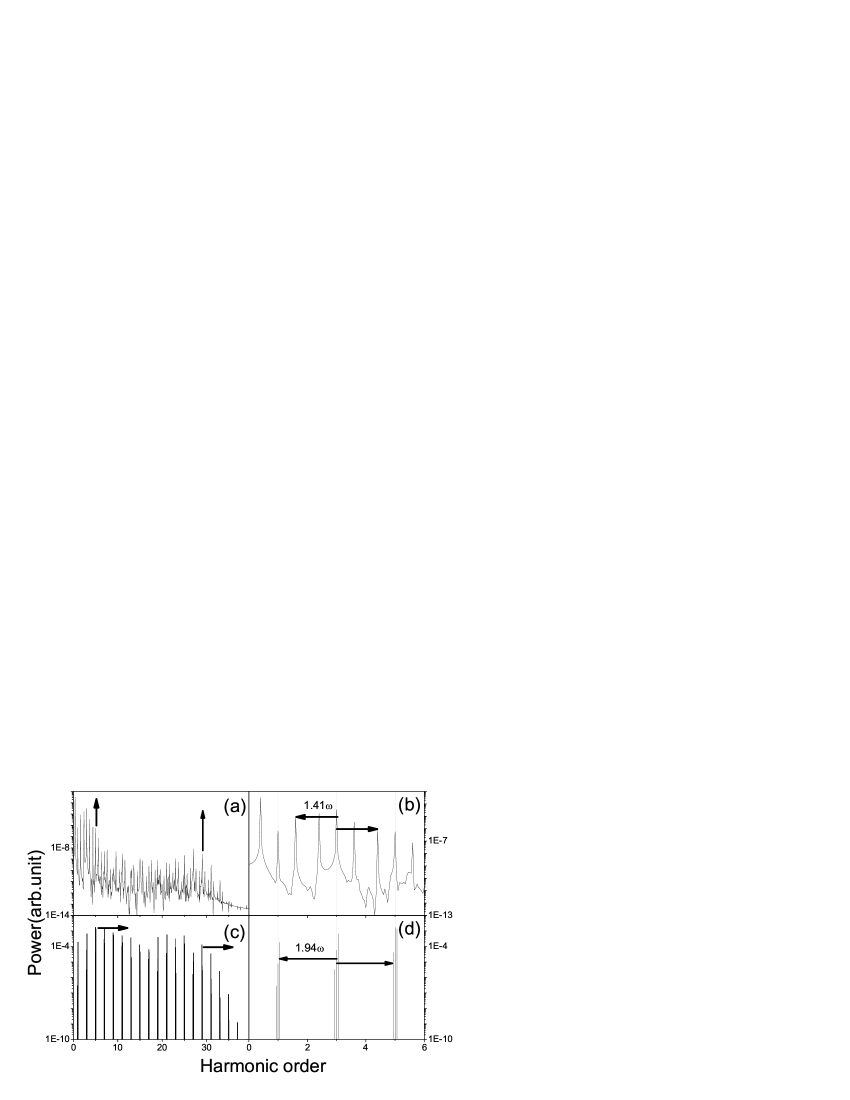
Figure 3: Harmonic-generation spectra at ${\omega}=0.05642a.u.$, $R=5.2$, $I=6.7\times 10^{13}W/cm^{2}$, initially in the ground state, from $1D$ time-dependent exact calculation ((a) and (b)) and the formula (14)((c) and (d)): (a) and (c) the contour of the spectrum; (b)and (d) the corresponding fine structure of (a) and (c), respectively. The arrows in (a) and (c) show the molecular and the atomic like cutoffs of the transfer harmonics; the arrows in (b)and (d) show the symmetrical splitting around the 3th harmonic, and the numbers above the arrows show the splitting separation.

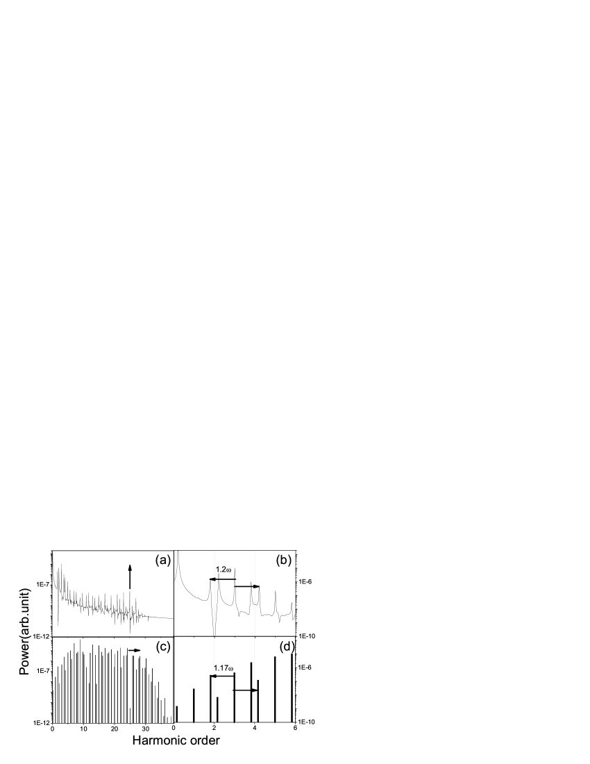
Figure 4: Harmonic-generation spectra at ${\omega}=0.05642a.u.$, $R=6a.u.$, $I=5.3\times 10^{13}W/cm^{2}$, initially in the ground state, from $1D$ time-dependent exact calculation ((a) and (b)) and the formula (14)((c) and (d)): (a) and (c) the contour of the spectrum; (b)and (d) the corresponding fine structure of (a) and (c), respectively. The arrows in (a) and (c) show the atomiclike cutoffs of the transfer harmonics; the arrows in (b)and (d) show the symmetrical splitting around the 3th harmonic, and the numbers above the arrows show the splitting separation.

Figure 5: The splitting separation(scaled by the frequency ${\omega}$) at ${\omega}=0.05642a.u.$ get from the model prediction of $Q$(solid curve) and from $1D$ time-dependent exact calculation (dotted curve) VS the maximum absolute amplitude of the external electric field (atomic unit): (a)$R=5.2$; (b) $R=6$.

Figure 6: Harmonic-generation spectra calculated from $1D$ time-dependent exact calculation((a) and (b)) and the formula (20) ((c) and (d)) at $R=8a.u.$, $I=6.7\times 10^{13}W/cm^{2}$ and ${\omega}=0.05642a.u.$, (a) and (c)initially in the ground state; (b) and (d)initially in the coherent superposition state of the ground state and the first excited state with equally weighted populations.The arrows in (a) and (c) show the atomic-like cutoffs of the transfer harmonics.

Figure 7: Harmonic-generation spectra (same parameters as in Fig.4), calculated from the formulas (10)-(13): (a)from (10); (b)from (11); (c)from (12); (d)from (13).

Figure 8: Harmonic-generation spectra (same parameters as in Fig.6(a)), calculated from the formulas (16)-(19): (a)from (16); (b)from (17); (c)from (18); (d)from (19).

Figure 9: Harmonic-generation spectra at ${\omega}=0.05642a.u.$, $R=16$, $I=1\times 10^{14}W/cm^{2}$, initially in the ground state: (a) $1D$ time-dependent exact calculation; (b) calculation according to the formula (20). The arrows in (a) and (c) show the atomic-like cutoffs of the transfer harmonics.

In this section, we apply our theory to concrete model and present numerical results. For convenience, we adopt an $1D$ symmetrical diatomic molecule model. The Hamiltonian of the model molecule studied here is $H(t)$=$-\frac{d^{2}}{2dx^{2}}$+$\frac{z}{\sqrt{1+({x+0.5R})^{2}}}$+$\frac{z}{\sqrt{1+({x-0.5R})^{2}}}$$-xE\sin({\omega}t)$, where $z$ is the effective charges, $R$ is the internuclear separation, $E$ is the absolute amplitude of the external electric field here and ${\omega}$ the frequency of the external field. In the paper, we adopt atom unit, $\hbar=e=m_{e}=1$, the laser intensity varies from $10^{13}W/cm^{2}$ to $10^{14}W/cm^{2}$($0.017a.u.-0.055a.u.$), the internuclear separation varies from intermediate $R$ ($5.2a.u.,$ and $6a.u.$) to large $R$ ($16a.u.$), the wavelength adopted is $\lambda$=$800nm$, accordingly ${\omega}=0.05642a.u.$ and the laser pulse contains 20 optical cycles. Numerically the above schrödinger equation can be solved by operator-splitting method22 .

We begin the calculation by assuming the electron initially is in the ground state. But Ivanov et al show that one should consider at least two wave packets excited to the electronic surfaces in their program32 , which means initially the system should be in the coherent superposition state21 . So we also perform the calculations from the coherent superposition state of the ground state and the first excited state with equally weighted populations.

III.1 Failure of the two-level modle in producing the whole harmonic spectrum

When $R=5.2a.u.$, the ionization potential of ground state is $E_{0}=-0.89830a.u.$ and first excited state is $E_{1}=-0.84085a.u.$. The energy separation between $E_{0}$ and $E_{1}$ is $\triangle E=0.05745a.u.$, which is in the near-(one-photon)-resonance region. Fig.1 shows the spectrum from $1D$ time-dependent calculation for the model molecule at $R=5.2a.u.$. In Fig.1, each odd harmonic peak is accompanied symmetrically by two strong sidebands. The energy separations between the neighboring sidebands all have the same value, which can be explained in a dressed molecule state picture33 .

Comparison between Fig.1 (a) and Fig.1(c) shows that while the external field becomes stronger and although the ground states and the first excited state depletion in Fig.1(c) is only $0.03$, there is very large difference between $1D$ time-dependent exact calculation and two-level calculation. So the continuum state effects on spectrum must be considered in this case. Otherwise, an obvious characteristic, different from atom, for the population of molecule states is the strong-coupling of the ground state and the first excited state. It shows that it is necessary and reasonable to consider the first excited state effect on harmonic generation to explain the spectrum from symmetrical diatomic molecular ions.

While $R=16a.u.$, the ionization potentials of the ground state and the first excited state are $E_{0}=-0.732574a.u.$ and $E_{1}=-0.7325723a.u.$, respectively. The energy separation is $\triangle E=1.7\times 10^{-6}a.u.$, which is in the strong-coupling region. When $I=10^{14}W/cm^{2}$, and the depletion of ground states and the first excited state is only $0.025$. Fig.2(b) exhibits harmonic-generation efficiencies of at least four orders of magnitude greater than that of Fig.2(a). It is worth it to be noted that both odd and even harmonic peaks appear although the even harmonic is weak in Fig.2, which accords with our above analysis that with the increasing internuclear separation $R$, the Rabi splitting of the odd harmonics should converge towards even harmonics and their intensity should become weaker and weaker. Again the calculation result also shows the strong-coupling of the ground state and the first excited state.

III.2 Harmonic spectrum calculated from our model

Fig.3(a) and (c) show the HOHG spectra from the $1D$ time-dependent calculation and the numerical calculation of the formula (14) with $R$=$5.2a.u.$ and assuming the system initially being in the ground state. Fig.3(b) and Fig. 3(d) show the fine structure of Fig.1(a) and Fig.3(c), respectively. The splitting separation is $Q=1.41w$ in Fig.3(b) and $1.94w$ in Fig.3(d). The discrepancy is due to invalidation of rotating-wave approximation in intense field. A plateau in low-order region is also identifiable in the spectrum in Fig.3(c) with a cutoff at the 5th harmonic order, which agrees with Fig.3(a). This corresponds to the maximum energy acquired by the electron in the two-level system in the presence of the field26 . Furthermore, a second plateau up to the $25th$ harmonic order which is associated with the ground-continuum coupling (referred to as the atomic plateau) can be identified. The cutoff position of the atomic plateau can be well explained by a semiclassical model28 .

Fig.4 shows the HOHG spectra from $1D$ time-dependent numerical calculation and (14) with $R$=$6a.u.$ and $E_{1}-E_{0}=0.0304a.u.$ The total depletion of the ground states and the first excited state is $0.34$. The splitting separations is $Q=1.2{\omega}$ in Fig.4(b) and $1.17{\omega}$ in Fig.4(d). The position of cutoff in Fig.4(c) is at the $24th$ harmonic order that agrees with the order $n=(3.17U_{p}+I_{p})/{\omega}$, the cutoff law predicted by the semiclassical mechanism of HOHG.

Fig5 shows the comparison of the splitting separation(scaled by the frequency ${\omega}$ with ${\omega}=0.05642a.u.$) between the model prediction of $Q$=$\sqrt{|Q^{2}_{R}|+\xi^{2}}$(solid curve) and the $1D$ time-dependent exact calculation (dotted curve) at $R$=$5.2a.u.$(Fig5(a)) and $R$=$6a.u.$(Fig5(b)). It is obvious that in the near resonance case(Fig5(a)), good agreement is obtained while the field is weak. However while the field becomes stronger, the difference between the theory one and the numerical one seems smaller in Fig5(b) than in Fig5(a) with the same field intensity.

III.3 Influence of initial condition and internuclear distance

At intermediate $R$, such as $R$=$5.2a.u.$ or $R$=$6a.u.$, no matter initially the system is in the ground state or the first excited state, or the coherent superposition state, no distinct difference is found in the spectra from numerical calculations. However at large $R$, the case is rather different. Fig.6 shows the comparison of harmonic generation spectrum calculated from different initial condition at $R$=$8a.u.$, where $E_{1}-E_{0}=0.0052a.u.$ and $Q=0.95{\omega}$. In Fig.6(b), where the system initially is in the coherent superposition state, even harmonics appear although they are weaker than the odd harmonics, however in Fig6(a), where the system initially is in the ground state, even harmonics hardly are distinguishable. The result validates our analysis for (20), which predicts that at large $R$ if the system initially is in the ground state, only odd harmonic can be produced , and if it is in the coherent superposition state, even harmonics also should be emitted although their strength should be weaker than the odd ones. If initially the system is in the excited state, the case is analogous with the ground state. Other calculations at $R$=$16a.u.$ from different initial conditions also show similar result. The position of cutoff in Fig.6(c) is at the $23th$ harmonic order, which agrees with the order $n=(3.17U_{p}+I_{p})/{\omega}$.

At intermediate $R$, with the same parameters as in Fig4, Fig.7 shows the comparison of contributions to harmonic from the four different terms (10)-(13). It can be seen that all of them give equivalent contribution to HOHG in this case.

At large $R$, with the same parameters as in Fig6(a), Fig.8 shows the comparison of contributions to harmonic from the four different terms (16)-(19) if initially the system is in the ground state. It is the term of $|0\rangle\rightarrow|\mathbf{p}\rangle\rightarrow|0\rangle$ that contributes mostly to HOHG in the case. Similarly, the calculation also shows that if initially the system is in the first excited state, the primary contribution to HOHG should come from $|1\rangle\rightarrow|\mathbf{p}\rangle\rightarrow|1\rangle$.

III.4 Cutoff law at large $R$

Fig.9 shows the spectra calculated by our analytic theory and $1D$ numerical simulation with $R$=$16.a.u.$. The main difference is that there are weak even harmonic peaks in Fig.9(a) but no even harmonic peaks in Fig.9(a). This is because $E_{1}-E_{0}=0$ has been adopted in the analytic formulation but actually these two states are not completely degenerated. The position of cutoff in Fig.9(b) is at the $35th$ harmonic order, which agrees with the order $n=(5.33U_{p}+I_{p})/{\omega}$ that is obtained by the semiclassical calculation considering complex trajectories. This is consistent with the finding that at very large $R$, the molecule has different cutoff law 2 ; 13 .

IV Conclusions

In summary, with considering the continuum states and ionization, the photon-emission spectra of the symmetric diatomic molecule ions in intense laser fields are thoroughly investigated and the role of the CR states is identified.

In the near-resonance region ($(E_{1}-E_{0})/{\omega}\simeq 1$), it is shown that the multiple Mollow triplet structure can be described by an analytic theory based on rotating-wave approximation and the Rabi oscillation between the ground state and the first excited state induces the symmetrical splittings of odd harmonics. The splitting separation in weak field can be approximately denoted by $Q$=$\sqrt{|ED|^{2}+(E_{1}-E_{0}-{\omega})^{2}}$.

In the strong coupling region ($(E_{1}-E_{0})/{\omega}\simeq 0$), all of the symmetrical splitting sidebands of odd harmonics gradually converge to even harmonics and their amplitudes get weaker and weaker with the increasing internuclear separation $R$. This is explained by our theory in the ultimate condition of $(E_{1}-E_{0})/{\omega}\simeq 0$($R\rightarrow\infty$). An interesting phenomenon is that in this case if initially the system is in the coherent superposition of the ground state and the first excited states, there are stronger even harmonics emitted than only in the ground or first excited state, and their intensity depends on the value of $|Q_{R}|=|ED|$.

In all above cases, the molecular plateau and the atomic plateau are identifiable in the analytical model and the cutoff positions are accordant with the numerical simulation and semiclassical calculation.

We also find that, for the symmetrical diatomic molecule, the dipole movement includes four terms, those are $|0\rangle\rightarrow|\mathbf{p}\rangle\rightarrow|0\rangle$, $|1\rangle\rightarrow|\mathbf{p}\rangle\rightarrow|0\rangle$, $|0\rangle\rightarrow|\mathbf{p}\rangle\rightarrow|1\rangle$ and $|1\rangle\rightarrow|\mathbf{p}\rangle\rightarrow|1\rangle$, respectively, denoting the transitions from the ground state or the first excited state to the continuum state, then back to the ground state or the first excited state. It is more complicated than atom case because of the existence of the $CR$ states. At intermediate $R$, each process contributes equivalently to molecular HOHG. However, at very large $R$, their contributions depend on the initial condition.

V Acknowledgements

This work is supported National Hi-Tech ICF Committee of China under Grant No. 2004AA84ts08 and the National Natural Science Foundations of China under Grant No. 10574019.

References

• (1) Liu$\_$Jie@iapcm.ac.cn
• (2) T. Kreibich, M. Lein, V. Engel, and E. K. U. Gross, Phys. Rev. Lett. 87, 103901(2001).
• (3) R. Kopold, W. Becker, M. Kleber, Phys. Rev. A 58, 4022(1998).
• (4) M. E. Sukharev, V. P. Krainov, Phys. Rev. A 62, 033404(2000).
• (5) P. Dietrich, M. Yu. Ivanov, F. A. Ilkov, and P. B. Corkum, Phys. Rev. Lett. 77, 4150(1996)
• (6) S. Chelkowski, A. Conjusteau, T. Zuo, and A. D. Bandrauk, Phys. Rev. A 54, 3235(1996).
• (7) Taiwang Cheng, Jie Liu, and Shigang Chen, Phys. Rev. A 62, 033402 (2000).
• (8) A. D. Bandrauk, S. Chelkowski, H. Yu, and E. Constant, Phys. Rev. A 56, R2537(1997).
• (9) H. Nikura et al., Nature(London)417, 917(2002).
• (10) A. D. Bandrauk, S. Chelkowski, and I. Kawata, Phys. Rev. A 67, 013407(2003).
• (11) M. Lein, N. Hay, R. Velotta, J. P. Marangos, and P. L. Knight, Phys. Rev. Lett. 88, 183903(2002); Phys. Rev. A 66, 023805(2002).
• (12) G. Lagmago Kamta and A. D. Bandrauk, Phys. Rev. A 70, 011404(R) (2004); G. L. Kamta and A. D. Bandrauk, Phys. Rev. A 71, 053407(2005).
• (13) X. X. Zhou et al., Phys. Rev. A 72, 033412(2005).
• (14) C. C. Chirila and M. Lein, Phys. Rev. A 73, 023410(2006).
• (15) R.Kopold, W.Becker,M.Kleber, Phys. Rev. A 58 4022 (1998).
• (16) Xi Chu and Shih-I Chu, Phys. Rev. A 63 023411 (2001).
• (17) X.M.Tong, and Shih-I Chu, Phys. Rev. A 61 021802 (2000).
• (18) C.C.Chirila and M.Lein,Phys. Rev. A 73 023410 (2006).
• (19) K.Miyazaki,M. Kaku, G. Miyaji, A. Abdurrouf, and F. H. M. Faisal,Phys. Rev. Lett. 95, 243903 (2005).
• (20) C.Vozzi, et al Phys. Rev. Lett. 95 15902 (2005), and references therein.
• (21) A. D. Bandrauk and Huizhong. Lu, Phys. Rev. A 68, 043408(2003).
• (22) Bingbing Wang, Taiwang Cheng, Xiaofeng Li, Panming Fu, Shigang Chen, and Jie Liu Phys. Rev. A 72, 063412 (2005)
• (23) Bambi Hu, Baowen Li, Jie Liu, and Yan Gu Phys. Rev. Lett. 82, 4224 (1999).
• (24) A. D. Bandrauk and M. L. Sink,Chem. Phys. Lett. 57, 569(1978); J. Chem. Phys. 74, 1110(1981).
• (25) M. Yu. Ivanov, P. B. Corkum, Phys. Rev. A 48, 580 (1993).
• (26) T. Zuo, S. Chelkowski, and A. D. Bandrauk, Phys. Rev. A 48, 3837(1993).
• (27) T. Zuo, S. Chelkowski, and A. D. Bandrauk, Phys. Rev. A 49, 3943(1994).
• (28) M. Lewenstein, Ph. Balcou, M. Yu. Ivanov, Anne L’Huillier and P. B. Corkum, Phys. Rev. A 49, 2117(1994).
• (29) P. B. Corkum, Phys. Rev. Lett. 71, 1994(1993).
• (30) H. R. Reiss, Phys. Rev. A 22, 1786(1980).
• (31) R. Bavli and H. Metiu, Phys. Rev. A 47, 3299(1993).
• (32) B. R. Mollow, Phys. Rev. 188, 1969(1969).
• (33) M. Yu. Ivanov and P. B. Corkum, Phys. Rev. A 48, 580(1993).
• (34) E. E. Aubanel, J. M. Gauthier, and A. D. Bandrauk, Phys. Rev. A 48, 2145(1993).