The self-energy of the electron: a quintessential problem in the development of QED

Abstract

The development of Quantum Electrodynamics (QED) is sketched from it’s earliest beginnings until the formulations of 1949, using the example of the divergent self-energy of the electron as a quintessential problem of the 1930’s-40’s. The lack of progress towards solving this problem led researchers to believe that after the conceptual revolution of quantum mechanics a new conceptual change was needed. It took a war and a new generation of algorithmically inclined physicists to pursue the conventional route of regularization and renormalization that led to the solution in 1947-1949. Some remarks on contemporary high energy physics are made.

1 Introduction

The beginning of the twentieth century saw two conceptual revolutions in physics that would dominate the theoretical physics of the entire century. The first was Einstein’s discovery of special and general relativity, that abruptly shook our conceptions of space and time. The lesson of special relativity was that we can no longer treat space and time as separate entities, but that they are intermixed and that no treatment can be totally satisfactory if it does not treat them on an equal footing. The second conceptual change was the development of quantum mechanics, that replaced the deterministic framework of classical physics by an essentially probabilistic one, that only allows us to calculate the probability of an event. These two theories were developed independently from each other (though often by the same researchers). Special relativity was completed in 1905 by Einstein. This was followed by ten years of labor on the general theory, which was presented by Einstein in 1916. Quantum mechanics began in 1901 with the black-body radiation of Planck, but needed more time to mature. The physicists that were concerned with it in those early days of the ‘old quantum theory’, Bohr, Einstein, Planck, were combining classical methods with new quantization principles and achieved some level of success. But the true breakthrough in quantum mechanics would only come when a new, younger generation of physicists stood up, who weren’t so deeply rooted in classical physics any longer, but had grown up with the new, revolutionary methods of quantum physics. These physicists like de Broglie, Heisenberg, Dirac and Pauli formulated quantum mechanics in the modern form in 1925-1927. Unlike Planck, Bohr and Einstein, who had used quantization methods in their calculations but had still arrived at exact predictions, the new theory could only give the probability of the outcome of an experiment. This conceptual change had remained out of reach for the old quantum theory and Einstein especially has never come to terms with it.

But the problems haunting physics were certainly not all resolved by the developments of the first decades of the twentieth century. The situation was that there were two theories, one describing the very fast (special relativity) and one pertaining to the very small (quantum mechanics). But electrons are very small particles that sometimes travel at speeds near the speed of light, and photons, the quanta of light that reappeared in quantum theory after hundreds of years of a wave picture of light, always travel at the speed of light. In these cases the two theories had to be applied both. As a consequence, the interaction of particles with the electromagnetic field was still poorly understood. This all constituted a great need to unify the two theories in a consistent framework. Immediately after the definite formulation of quantum theory, this new exploration was embarked upon.

The problems were however hard to resolve. Firstly there were two possible ways to construct the new theory: quantization of the involved fields or searching for a covariant theory of particles. The first line of research was the most popular and it started with de Broglie, and then moved on past the wave mechanics of Schrödinger to the work of Jordan, Pauli and Heisenberg. Their quantization methods for fields gave rise to new phenomena, such as the creation and annihilation of particles, which was a new phenomenon, as the number of particles is a conserved quantity in ordinary quantum mechanics. Dirac, however, followed the path of the particles and gave a covariant equation for the behavior of the electron. One of the consequences thereof was the existence of anti-particles. Much bigger than these early successes were the problems of the theory. It was littered with divergences, all kinds of relevant quantities came out infinite in the theory.

The physicists that worked on quantum electrodynamics in the 1930’s were the physicists that had accomplished the big conceptual breakthrough of quantum mechanics in the 1920’s. When overwhelmed by the problems posed to them by quantum electrodynamics, they quickly turned away from the methods they were using and started looking for a new conceptual change. They were very pessimistic about finding a solution to the problem of the divergences of the theory in the existing framework and believed that new conceptual change was needed to surpass the difficulties.

However, this was not what happened. The second world war started at the end of the 1930’s, which paralyzed research and destroyed the research infrastructure in Europe. In the meantime a new generation of American physicists was trained in the American research laboratories, for whom physics was all about numbers. In these research facilities the line between experiment and theory was a fine one, especially when compared to European research centers. These physicists were all drafted to work in war laboratories, mostly the Manhattan project and the development of the Radar, which gave them a strong focus on their problem-solving and algorithmic capabilities. After the war these young physicists quickly found the solution of the problems of quantum electrodynamics. The methods they used were conventional rather than revolutionary and the expected conceptual change did not take place. Their solution consisted of regularization and renormalization and succeeded in discarding the infinities that had troubled the theory so much. The fact that it took these physicists to find the solution is found in their training during the war. Both research paths (field and particle) came to a theory (found respectively by Julian Schwinger and Richard Feynman) and not long after, these two approaches were shown to be equivalent (by Freeman Dyson).

In the following sections of this papers this whole evolution will be illustrated by reconstructing the development of one of the quintessential problems of the early quantum electrodynamics, that of the self-energy of the electron. This is one of the numerous divergences that haunted the theory from the start and was given much attention during the subsequent developments. When the final solution was falling into place both Schwinger and Feynman considered this problem as one of the first of their new theory (in their papers ?, ?, ?, ?). We shall see how this problem showed up after the development of quantum mechanics and what were the different attempts at solving it. Some attention will go to the attempts at conceptual change of the 1930’s. Then we will follow the younger physicists during the war and sketch how they came to the final solution.

In the final section it will be argued that the situation of the development of quantum electrodynamics is somewhat similar to the present situation in theoretical high energy physics and this point will be elaborated upon a bit more.

2 The global problem: a covariant quantum mechanics

As has been said before, the problem with quantum mechanics was that it didn’t agree with the principle of relativity of Einstein’s theory, i.e. neither Schrödinger’s wave mechanics nor Heisenberg’s matrix mechanics was covariant. This is immediately clear when we consider the Schrödinger equation for a mechanical particle without spin

$$i\hbar\frac{\partial}{\partial t}\psi=H\psi\quad;\quad\psi\in\mathcal{H}=L^{2}(\mathbb{R}^{3})\ ,$$ (1)

here the Hamiltonian $H$ is

$$H=-\frac{\hbar^{2}}{2m}\Delta+V(x)\ .$$ (2)

This gives a differential equation of first order in the time derivative and of second order in the place derivative, which can’t be Lorentzcovariant, as space and time have to be treated equally in special relativity. A covariant version of the Schrödinger equation had to be found.

2.1 The first attempt: the Klein-Gordon equation

The first covariant quantum mechanical equation was found by using the correspondence principle of quantum mechanics together with the new insights relativity had brought. The correspondence principle is a way to quantize classical equations, by changing space coordinates $x_{k}$ by multiplication operators on the state space $\mathcal{H}=L^{2}(\mathbb{R}^{3})$. On a wave function this gives $\psi(x)\rightarrow x_{k}\psi(x)$. The classical momenta $p_{k}$, however, are replaced by differential operators: $\psi(x)\rightarrow\frac{\hbar}{i}\frac{\partial}{\partial x_{k}}\psi(x)$. The classical energy is substituted by the energy-differential operator $i\hbar\frac{\partial}{\partial t}$. By making these changes, one becomes the Schrödinger equation out of the classical expression for the energy of a particle ($E=\frac{p^{2}}{2m}+V(x)$), as one can readily check.

In special relativity space and time coordinates are considered together and they form covariant vectors $(x_{\mu})=(x_{0},x_{1},x_{2},x_{3})$ and $(p_{\mu})=(p_{0},p_{1},p_{2},p_{3})$ (here $x_{0}=ct$ and $p_{0}=E/c$). The correspondence principle connects these two vectors

$$p_{\mu}=i\hbar\frac{\partial}{\partial x^{\mu}}$$ (3)

which gives again

$$p_{0} =\frac{E}{c}=i\hbar\frac{\partial}{c\partial t}$$ (4)

$$p_{k} =\frac{\hbar}{i}\frac{\partial}{\partial x_{k}}\ .$$ (5)

In special relativity the expression for the energy of a free particle is given by

$$E^{2}=m_{0}^{2}c^{4}+p^{2}c^{2}\ .$$ (6)

This gives

$$m_{0}^{2}c^{2}=\frac{E^{2}}{c^{2}}-p\cdot p=p^{\mu}p_{\mu}$$ (7)

(Einstein summation convention). By quantizing this equation we find the simplest covariant quantum mechanical equation, the Klein-Gordon equation for a free particle with spin zero:

$$p^{\mu}p_{\mu}\psi=m_{0}^{2}c^{2}\psi\quad,\psi\in\mathcal{H}$$ (8)

or by substitution

$$\Big{(}\square+\big{(}\frac{m_{0}c}{\hbar}\big{)}^{2}\Big{)}\psi=0$$ (9)

with the d’Alembertian given by

$$\square=\partial^{\mu}\partial_{\mu}=\frac{\partial^{2}}{c^{2}\partial t^{2}}-\sum_{k=1}^{3}{\frac{\partial^{2}}{\partial x_{k}^{2}}}\ .$$ (10)

So we see that as the Schrödinger equation is the quantization of the classical expression for the energy of a particle, the Klein-Gordon equation is the quantization of the relativistic expression for the energy. When we solve this Klein-Gordon equation, we find solutions with positive energies as well as solutions with negative energies. This shouldn’t be surprising, because the relativistic expression for the energy of a particle (6) has always positive and negative solutions. In quantum mechanics these negative solutions give interpretation difficulties (non-positiveness of the probability densities).

2.2 Staring into the fireplace: the Dirac equation

One night Dirac was staring into a fire when he suddenly thought he wanted a relativistic wave equation that was linear in the space-time derivatives $\partial_{\mu}\equiv\frac{\partial}{\partial x^{\mu}}$. This equation had to have the form of ‘some linear combination of the $\partial_{\mu}$’s working on a field $\psi$, that is equal to a constant times that field’. When we write this down, this becomes

$$(i\gamma^{\mu}\partial_{\mu}-m)\psi=0\ .$$ (11)

If the $\gamma^{\mu}$’s were numbers, the vector $\gamma^{\mu}$ would define a direction in space-time and this would break the covariance of the theory. This is why the $\gamma^{\mu}$’s can’t be numbers. They were identified as matrices, subjected to the anti-commutation relation

$$\{\gamma^{\mu},\gamma^{\nu}\}=2\eta^{\mu\nu}\ ,$$ (12)

with $\eta^{\mu\nu}$ the Minkowski metric of special relativity. The wonderful thing about this equation is that it describes the spin property of electrons, which is a purely quantum mechanical effect. This is the equation for the behavior of spin-1/2 particles.

The Dirac equation, just like the Klein-Gordon equation, has negative energy solutions that cause problems. Dirac then proposed to consider as the vacuum state that state in which all negative energy states are filled. Then the Pauli exclusion principle will force any extra electron to take a positive energy state. This vacuum state is called the sea of electrons. When an electron is excited from a negative energy state to a positive energy state, it leaves a hole in the sea behind. Dirac proposed that this hole be considered a particle itself, with a positive charge now. First he identified this particle with the proton, but subsequent developments showed that this couldn’t be the case. He then proposed that it was a new particle, identical to the electron but for its charge, which was $+e$. He called it the positron. The positron was experimentally observed in 1932 by Carl D. Anderson. This way of looking at the sea of electrons allows us to view pair creation as an electron jumping from a negative energy state to a positive energy state, leaving a hole, i.e. a positron, behind. This theory became known as Dirac’s hole theory.

3 The problem: the divergence of the self-energy of the electron

The self-energy is the energy that an electron in free space, isolated from other particles, fields, or lightquanta, possesses. In the classical theory it posed no problem, but after the development of quantum theory, it became a critical problem for theoretical physics. The problem was first noted by Pauli and Heisenberg in their papers ?, ?, ?, ?. In ?, ? Weisskopf gives a good review of the problem. The self-energy of the electron is given by

$$W=T+(1/8\pi)\int(E^{2}+H^{2})\mbox{d}V\ ,$$ (13)

with $T$ the kinetic energy of the electron (which for a non-moving electron is just equal to the rest-energy $mc^{2}$) and $E$ and $H$ the electric and magnetic field strengths. d$V$ is the volume-element.

In classical electromagnetism, the electric field $E$ of a free electron is equal to $e/r^{2}$, $r$ is the distance to the electron. When we assume that the electron does not have any spin, the magnetic field $H$ equals zero. The self-energy is then given by

$$W\sim mc^{2}+\int\frac{e^{2}}{r^{4}}\mbox{d}V\sim mc^{2}+\int\frac{e^{2}}{r^{2}}\mbox{d}r\ .$$ (14)

If the radius of the electron were zero, this integral would run from zero to infinity and thus constitute a linear divergence. When we assume that the electron has a radius equal to $a$, the integral is calculated to be $\int_{a}^{\infty}e^{2}\mbox{d}r/r^{2}=e^{2}/a$. This is the reason why classically it was assumed that the electron has a finite radius, and thus isn’t a point particle.

The development of quantum mechanics made the self-energy, however, into a critical problem. We can discern three reasons for this:
(a) Quantum mechanics shows that the radius of the electron has to be zero, i.e. that the electron is a point particle. This is because we can prove that the product of the charge densities in two different points equals a delta-function, i.e. a function that peaks in one place and is equal to zero everywhere else. For a free electron this means that the probability that we find charge densities in two different places equals zero. Thus the charge has to be concentrated in one point. Like we saw in the last paragraph this means that the contribution of the electrostatic energy diverges. This divergence is linear.
(b) Relativistic quantum mechanics showed that the electron possesses an intrinsic spin (which was first experimentally observed by Stern and Gerlach). Because of this intrinsic spin-property of the electron, the value of $H$ will not be equal to zero anymore, as the spin induces a magnetic field and an alternating electric field. These contributions to the self-energy thus have to be added to that of the electrostatic energy.
(c) Finally, quantum mechanics of the electromagnetic field postulates the existence of field strength fluctuations in free space. The divergence of the self-energy as a consequence of these fluctuations is bigger than that of the electrostatic energy. The energy of the fluctuations is $W_{\mbox{fluct}}\sim e^{2}h/mca^{2}$ for an electron of radius $a$. This constitutes a quadratic divergence.

4 The self-energy in Dirac’s one-particle theory

The first calculation of the self-energy of the electron was performed using Dirac’s one-particle theory. This is the theory that uses the Dirac equation, but doesn’t use the vacuum state with all negative energy states filled, as does Dirac’s hole theory. The calculation uses standard quantum mechanical perturbation theory to find the $e^{2}$-contribution to the self-energy. The whole Hamiltonian of the system is split into the Hamiltonian of the unperturbed system $H_{0}$ (here the Hamiltonian of the free electron and the Hamiltonian of the free electromagnetic field) and the interaction Hamiltonian $H^{\prime}$ (here the interaction of the electron with the electric field). It is assumed that the contribution of the interaction Hamiltonian is small compared to the contributions of the unperturbed system. The Hamiltonian of Dirac’s one-particle theory is given by

$$H =H_{0}+H^{\prime}$$ (15)

$$=\sum\hbar kca_{k\mathbf{\epsilon}}^{*}a_{k\mathbf{\epsilon}}+H_{\mbox{Coulomb}}+\beta m+\alpha\cdot(\mathbf{p}-e\mathbf{A})$$ (16)

with the interaction term linear in A:

$$H^{\prime}=-e\alpha\cdot\mathbf{A}\ ,$$ (17)

with $\mathbf{A}$ the vector potential of electromagnetism and $\alpha$ satisfying

$$\alpha_{i}\alpha_{j}+\alpha_{j}\alpha_{i}=\delta_{ij}\ .$$ (18)

The first contribution to the self-energy of the electron is then given by

$$\Delta W=\sum{\frac{|<n|H^{\prime}|0>|^{2}}{E_{0}-E_{n}}}\ ,$$ (19)

from standard perturbation theory. $|n>$ are the unperturbed states of $H_{0}$. We have

$$E_{0}-E_{n}=m\mp\sqrt{m^{2}+k^{2}}-k\ ,$$ (20)

which for large $k$ goes like $m$. The matrix element from the numerator is for large $k$

$$|<n|H^{\prime}|0>|^{2}\sim\frac{e^{2}}{k}\ .$$ (21)

Since we can replace the sum by an integral

$$\sum_{n}\rightarrow\int\mbox{d}^{3}k\sim\int_{0}^{\infty}k^{2}\mbox{d}k\ ,$$ (22)

we find

$$\Delta W\sim\int\frac{k\mbox{d}k}{m}\ ,$$ (23)

which is a quadratic divergence. This situation is far worse than that in the classical theory, where, as we saw, we only have a linear divergence of the self-energy. ?, ? was the first to find this result. ?, ? and ?, ? came to similar conclusions.

In figure 1 we see this situation graphically. On the left we see a free electron at rest. A virtual photon appears, which forces the electron to have a momentum equal to $-k$, because of the conservation of momentum. This photon disappears and the electron is at rest again.

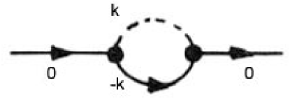
Figure 1: The self-energy of the electron to first order. On the left the electron is at rest. Then a virtual photon forms. On the right, the electron is at rest again.

5 Weisskopf’s calculation of the self-energy in Dirac’s hole theory

5.1 1934: calculation of the $e^{2}$ contribution

?, ?b used Dirac’s hole theory to calculate the self-energy of the electron to first order . He divided the total self-energy in an electrostatic part $E^{S}$ and an electrodynamic part $E^{D}$. He was able to show that the contribution of the electrostatic part only constituted a logarithmic divergence, which was better than what we just found using one-particle theory. For the electrodynamic part, however, he found, just as in one-particle theory, a quadratic divergence.

Not much later he received a letter from Furry, who reported to him that he had done the calculation of the self-energy in hole theory himself and had only found a logarithmic divergence for the electrodynamic part. Weisskopf readily admitted that he had made a mistake and published a correction ?, ?a. Let’s recall the most important results found in this paper. One particle theory led to

$$E^{S} =\frac{c^{2}}{h}\int_{0}^{\infty}\mbox{d}k+\mbox{finite terms}$$ (24)

$$E^{D} =\frac{e^{2}}{h}\Big{[}\frac{m^{2}c^{2}}{p(m^{2}c^{2}+p^{2})^{1/2}}\log\frac{(m^{2}c^{2}+p^{2})^{1/2}+p}{(m^{2}c^{2}+p^{2})^{1/2}-p}-2\Big{]}\int_{0}^{\infty}\mbox{d}k$$

$$\ \ +\frac{2e^{2}}{h(m^{2}c^{2}+p^{2})^{1/2}}\int_{0}^{\infty}k\mbox{d}k\ .$$ (25)

The divergence of the total self-energy is thus quadratic. In hole theory the following expressions were found

$$E^{S} =\frac{e^{2}}{h(m^{2}c^{2}+p^{2})^{1/2}}(2m^{2}c^{2}+p^{2})\int_{k_{0}}^{\infty}\frac{\mbox{d}k}{k}+\mbox{finite terms}$$ (26)

$$E^{D} =\frac{e^{2}}{h(m^{2}c^{2}+p^{2})^{1/2}}(m^{2}c^{2}-\frac{4}{3}p^{2})\int_{k_{0}}^{\infty}\frac{\mbox{d}k}{k}+\mbox{finite terms}\ .$$ (27)

This is only a logarithmic divergence of the $e^{2}$ term.

These results, however, could not be satisfactory. Heisenberg repeated the calculation himself and found the same results, but in a letter to Weisskopf he characterized this solution as “implausible and suspicious” (cited in ?, ?). The reason for this was that because of relativistic invariance reasons, one would expect an expression of the following form

$$E^{S}+E^{D}=\mbox{constant}\frac{e^{2}}{h}\sqrt{m^{2}c^{2}+p^{2}}\int\frac{\mbox{d}k}{k}\ ,$$ (28)

as the expression $m^{2}c^{2}+p^{2}$ is relativistically invariant, whereas the sum of the expressions in (26-27) is not. The lack of correct relativistic invariance was the biggest problem in pre-war quantum electrodynamics.

5.2 1939: logarithmic divergence of the full self-energy

The most extensive treatment of the problem of the self-energy of the electron before the second world war was given in 1939 by Weisskopf. In ?, ? he argued that the self-energy is logarithmic divergent in every order in hole theory. This was a major breakthrough. In 1936 Dirac, Heisenberg and Weisskopf had solved the problem of the vacuum polarization by using relativistically invariant subtraction principles and charge renormalization. Kramers, Pauli and Fierz had, in addition, already given a procedure to get rid of logarithmic divergences in 1937-1938. Weisskopf even went as far as to claim that all divergence problems in quantum electrodynamics could be solved by using these principles (?, ?).

But these new insights were never brought together to construct a diver-
gence-free hole theory, not even up to first order. This was most probable because the physics community in the thirties did not believe that this was the right way to go and because serious questions were being asked about the methods to get rid of the infinities. As a reaction to a paper of ?, ? that introduced methods to solve problems with infinities, ?, ? questioned the uniqueness of the methods to subtract infinities, precisely because they are infinite. Pauli reacted shocked to a similar attempt by Heisenberg. Pauli noted that he didn’t believe that these methods to get rid of infinities could lead to results that were not already known.

The first attempts to come to a renormalization procedure were thus not met with a lot of enthusiasm by the European physics community. A unified theory of radiation remained an open problem.

6 Looking for conceptual change

All the attempts in the 1930’s to solve the problem of the divergences failed. This had much to do with the pessimism of the leading figures in physics. Bohr, Pauli, Dirac and Heisenberg didn’t see how the problem could be solved in the framework of quantum mechanics. They thought that the solution would come from new concepts, in the same manner as the problems of the old quantum theory were solved by introducing a whole new framework, i.e. the probabilistic quantum mechanics. As early as 1930 in an article concerning the self-energy of the electron, ?, ? remarked that the problem of the divergence of the self-energy does not appear in a lattice-world, i.e. a discrete model of space-time. He doesn’t elaborate on it any further there, because he immediately sees the difficulties of this proposal, most notably that a lattice breaks relativistic invariance.

In 1938 Heisenberg is still defending conceptual renewal. In ?, ? he claims that after the light speed $c$, that became a fundamental unit in relativity theory, and after Planck’s constant, which rose to prominence in the quantum mechanical revolution, the time has come for a new fundamental constant, a fundamental length now, that would delineate the area of validity for the classical theories, where the theory of fields and particles can be applied without difficulties, and below which new phenomena will appear. He regards the self-energy of the electron as one of the reasons for such a fundamental length.

Many other alternative formalisms were developed at the end of the 1930’s. Wheeler suggested that the formalism of state vectors and quantum fields should be replaced by a formalism based on observables only, such as the $S$-matrix he introduced in 1937. This $S$-matrix contains scattering amplitudes (the $S$-matrix became a vital part of modern quantum mechanics later, and Feynman gave easy rules to calculate its elements up to any desired order in perturbation theory, see infra). Wheeler and Feynman also worked on a formalism that sought to eliminate the electromagnetic field, by deriving all electromagnetic properties by an interaction at a distance. Dirac, radically, suggested the use of states of negative probability.

This looking for conceptual change held the clear development of a renormalization theory for divergences back, when all the ingredients to found it were already available. When the second world war broke out, the research was freezed and when it was finally over, the research climate had changed considerably. The center of post-war physics was no longer situated in Europe, but had moved to the United States, and the solution that hadn’t been possible in pre-war Europe, was found by a new generation of physicists.

7 Physicists in the second world war

The second world war brought great changes with it. European research was completely paralyzed and lots of European physicists emigrated to the United States (viz. Einstein, Wigner). Many physicists were set to work in the war effort. This included projects like the Manhattan project and the development of the Radar. Many of the developments in later quantum electrodynamics came out of the efforts of physicists that had worked in those war laboratories. The head of the Manhattan project was Oppenheimer and leading the theoretical division of the Los Alamos laboratory was Hans Bethe, who would play an important part in the post-war developments. At the Los Alamos laboratory we also find a young Richard Feynman. He worked in the computation facilities and he designed methods to do the great amounts of calculations that were necessary for the development of the nuclear bomb.

At the radiation laboratory at MIT we find Julian Schwinger during the war, doing theoretical work concerning the radar. The insights he gained there about radiation, he would apply to quantum mechanics after the war. Freeman Dyson was working as an analyst for a British fighter plane division.

We see that a lot of theoretical physicists were working on practical applications of their work during the war. This work was focussed on problem-solving and very quantitative by nature. This way they developed crucial skills for solving the problems of quantum electrodynamics. The problem-solving and algorithmic nature of the work of Feynman at Los Alamos, would show in his subsequent work on quantum electrodynamics. He would give a simple algorithm to solve problems in it.

This emigration of prominent physicists to the United States and especially the experience the young American physicists gained during the war, shifted the center of scientific research after the world war to the United States. Schwinger, Feynman and Dyson (and Tomonaga in Japan) would solve the problems that had troubled physicists during the 1930’s in two different ways, which turned out to be equivalent. Thus they found the most accurate theory known as yet.

8 1947-1950: Renormalization

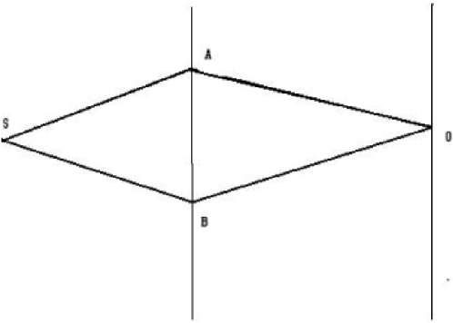
Figure 2: The two slit experiment.

During the years 1947-1950 Schwinger and Feynman both found a formalism which transformed quantum electrodynamics into a sound, divergence-free theory. The method of Schwinger was tedious and complicated, whereas Feynman’s gave a simple method to solve problems concerning radiation. We shall succinctly describe Feynman’s formalism and see how he uses it to work on the self-energy of the electron. It all begins with a reformulation of quantum mechanics.

8.1 Feynman’s path-integral formulation of quantum mechanics

We can illustrate the reformulation that Feynman gave of the quantum mechanics of Schrödinger, Heisenberg and Dirac by way of a familiar example. One of the most famous experiments in quantum mechanics is certainly the double-slit experiment. This experiment was first performed by Young for the case of light waves. These were sent to a screen in which two slits were made, and observed on a screen situated behind this first screen (see figure 2). The observation Young made was that these two rays interfered and this was thought to be a sufficient proof for the wave character of light. In quantum mechanics, however, we have wave-particle duality, such that when we sent particles to a screen with two slits, we will also find an interference pattern on the observation screen. This is because we have to add the amplitudes of the two electron paths and square them to get the probability (in Born’s interpretation of the Schrödinger equation). So in figure 2 we have two paths, we simply add the amplitudes of these two paths and square this sum.

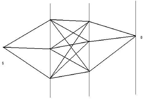
Figure 3: Various possibilities.

We can now ask what happens when we drill an extra hole in the middle screen. The solution is simple: we add the amplitude of the third path to the sum of the first two and square this expression to get the probability. We can also ask what happens when we add another screen, with a couple of holes drilled in it. This gives us the situation of figure 3. Now we have to add the amplitudes of all the possible paths shown and square this whole expression. This process can go on. When we add a fourth, a fifth screen, when we drill a fourth, a fifth hole in each screen, we always have to consider all possible paths and add amplitudes. When we add an infinity of screens, the whole space will be filled, when we drill an infinity of holes in a screen, the screen will disappear. This way we finally see that we have to add the amplitudes of all possible paths between s and o that the particle can take (see figure 4). This is the possible-paths interpretation of quantum mechanics of Feynman.

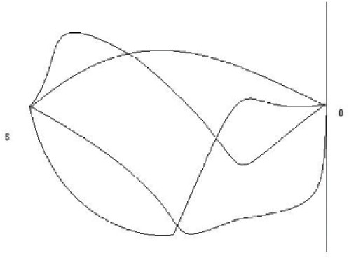
Figure 4: All possible paths.

Of course, this has to be formalized, and when we do this we get an integral over all possible paths, with the amplitude of a path given by $e^{iS}$, with $S$ the classical action of the path, which is given by an integral over the kinetic energy minus the potential energy of the particle (this last sum is the Lagrangian $L$). We find that the probability is given by the expression

$$\int{Dq(t)e^{i\int_{0}^{T}{dtL(\dot{q},q)}}}$$ (29)

8.2 The self-energy of the electron in Feynman’s QED

When we use this formulation and replace the classical action by a relativistic invariant one for fields, we become a quantum field theory. We can do this for fields described by the Klein-Gordon equation as well as for fields described by the Dirac equation. The problem then reduces to calculating the integral (29). It is, however, not possible to calculate this integral exactly, so it has to be calculated approximately, by expanding it in orders of the coupling constants (for quantum electrodynamics this is the fine-structure constant $\alpha=\frac{e^{2}}{\hbar c}\approx 1/137$). Feynman gave simple rules to construct the terms in this expansion for a given problem. One simply draws the situation one would like to calculate, for example the $e^{2}$ contribution leads to the diagram 1, and then the Feynman rules tell us how to associate expressions with these particles, lines and nodes. For the matrix-element of the $e^{2}$ contribution to the self-energy we get the following, complicated expression

$$e^{2}\int{\frac{\mbox{d}^{4}k}{(2\pi)^{4}}}\frac{\bar{u}^{r^{\prime}}(p)}{(2\pi)^{3/2}}\Bigg{(}\frac{m}{p_{0}}\Bigg{)}^{1/2}\cdot\frac{i}{(2\pi)^{4}}\frac{\not{p}-\not{k}+m}{(p-k)^{2}-m^{2}+i\varepsilon}\cdot\frac{-ig_{\mu\nu}}{k^{2}+i\varepsilon}$$

$$\Bigg{(}\frac{1}{2\pi}\Bigg{)}^{4}i^{2}\gamma_{\mu}\gamma_{\nu}\cdot\frac{u^{r}(p)}{(2\pi)^{3/2}}\Bigg{(}\frac{m}{p_{0}}\Bigg{)}^{1/2}\ ,$$ (30)

but what is important is that this behaves as

$$\int{\mbox{d}^{4}k\frac{\not{k}}{k^{4}}}$$ (31)

for large $k$.

Thus it seems that we have a linear divergence. Because of the symmetry of the integral, however, this contribution vanishes, which leads to a logarithmic divergence.

?, ? is able to show, using this formalism, that the first order correction to the self-energy of the electron is finite. He uses a modification of quantum electrodynamics, in which the Dirac-function that appears in his expression, is replaced by a function of small width and great height (that thus approximates a Dirac-function). This way he avoids the divergence coming from this singularity.

As his solution is long and tedious, it is perhaps more instructive to give some cursory remarks regarding the process of regularization and renormalization. For example, we can solve a logarithmic divergence by this procedure as follows. Regularization states that one should not expect this theory to hold to arbitrarily high energies, the theory only holds up to some value for the energy, say $\Lambda$. This transforms the integral to

$$\int^{\Lambda}{\mbox{d}^{4}k\frac{1}{k^{4}}}\ .$$ (32)

We can interpret this $\Lambda$ as the value at which the expansion is not valid anymore. At the value $\Lambda$ the second term in the expansion becomes as large as the first term. Then one can not claim any longer that this expansion will give accurate results. This drops the infinities, but we do introduce a new, unknown constant $\Lambda$.

Here comes renormalization into play. What we measure are of course physical quantities. When we couple theory to experiment, we have to express the theoretical results in terms of the physical couplings. When we do this we see that the constant $\Lambda$ vanishes from the expressions.

For instance, using the example of vacuum polarization, we see that this polarization effects the charge density of the electron. That way, it changes the charge of the electron, because the charge is the integral over the charge density. As a consequence, the charge of the electron will not longer equal $e$. When we now want to express results of vacuum polarization, we shouldn’t use $e$, which is the theoretical coupling, but the physical coupling, i.e. the changed value of the charge. Expressing the theoretical results by using the physical couplings rather than the theoretical ones, produces finite results (since the infinities cancel in the process of rewriting the expressions in terms of the physical couplings).

9 Conclusion

We have seen how applying quantum mechanics to the interaction between fields and particles led to problems that were apparently out of reach of the quantum theory. The theory that was developed in the thirties of the previous century, was haunted by a lot of divergences, that couldn’t be of a physical nature. The European physicists had no trust in the methods used up to then and thought that only a new conceptual change could lead to a solution of these problems. It took a new generation of American physicists, trained with a strong emphasis on the algorithmic and problem-solving aspects of physics, to see that the solution could be found in a conventional manner, by disposing of the divergences by renormalization. This way they developed quantum electrodynamics, and more generally, quantum field theory.

In the 1950’s and 1960’s quantum field theory was developed further and applied to the other forces of nature. Using gauge theories a unification of all known forces except gravity was achieved. Weinberg, Salam and Glashow unified the electromagnetic force with the weak nuclear force using quantum field theory. The strong nuclear force was described as a quantum field theory in quantum chromodynamics (QCD). This eventually led to the grand unification theories (GUT’s) that unified these three forces in one consistent framework.

The only remaining force that eluded the quantum mechanical framework was gravity. A quantum field theory for gravity can not be renormalizable. Emphasis in the last twenty years of the twentieth century in high-energy physics was on the problem of finding this quantum description and unifying all forces in one theory. Highest hopes in the theoretical physics community rest on string theory. This theory is founded on the principles of quantum field theory, but the basic entities aren’t particles anymore, but one-dimensional strings. It is hoped that this field theory will give a consistent quantum description of gravity. String theory has as virtues that it naturally contains a spin-2 particle, a particle that can function as the graviton, the messenger-particle of gravity and that it provides a framework to unify all four forces of nature. String theory, however, has still a lot of problems. For instance, it predicts that space-time has ten dimensions, instead of the usual four. The search for the solution of these problems already takes up a few decades.

In certain aspects, the situation we see today is similar to the situation that confronted physicists in the 1930’s. The problem then was unifying the theory of special relativity with the quantum theory, and the problem today is unifying the theory of general relativity with the quantum theory. The problems then, the divergences, seemed unsolvable, and the problems today again make the physical interpretation of the theory difficult, e.g. the extra dimensions. The manner in which a solution is sought, however, is completely different. The leading physicists of the 1930’s had brought about the conceptual change of quantum theory and believed that only a new conceptual change could lead to satisfying results. We saw that this judgement was mistaken. The physicists that started the research for a quantum mechanical description of gravity in the second half of the twentieth century, were physicists who had accomplished many successes with quantum field theory. It was only natural for them to look for a solution using the framework of quantum field theory, which led them to string theory. However, now that we see that this theory does not arrive at a solution, we may ask whether it could not be that this time we do need a conceptual change.

References

- DiracDirac Dirac, P. A. M. (1934). Discussion of the infinite distribution of electrons in the theory of the positron. Proceedings of the Cambridge Philosophical Society, 30, 150-163. (Reprinted in (?, ?))
- FeynmanFeynman Feynman, R. P. (1949). Space-time approach to Quantum Electrodynamics. Physical Review, 76, 769. (Reprinted in (?, ?))
- HeisenbergHeisenberg Heisenberg, W. (1930). Die Selbstenergie des Elektrons. Zeitschrift für Physik, 65, 4-13. (Reprinted in English translation in (?, ?))
- HeisenbergHeisenberg Heisenberg, W. (1938). Über die in der theorie der Elementarteilchen auftretende universelle Länge. Annalen der Physik, 32, 20-33. (Reprinted in English translation in (?, ?))
- Heisenberg PauliHeisenberg Pauli Heisenberg, W., Pauli, W. (1929). Zur Quantendynamik der Wellenfelder. Zeitschrift für Physik, 56, 1-61.
- Heisenberg PauliHeisenberg Pauli Heisenberg, W., Pauli, W. (1930). Zur Quantentheorie der Wellenfelder. II. Zeitschrift für Physik, 59, 168-190.
- MillerMiller Miller, A. I. (1994). Early Quantum Electrodynamics: A source book. Cambridge University Press.
- OppenheimerOppenheimer Oppenheimer, J. (1930). Note on the theory of the interaction of field and matter. Physical Review, 35, 461.
- PeierlsPeierls Peierls, R. (1934). The vacuum in Dirac’s theory of the positive electron. Proceedings of the Royal Society (A), 146, 420-441.
- RosenfeldRosenfeld Rosenfeld, L. (1931). Zur Kritik der Diracschen Strahlungstheorie. Zeitschrift für Physik, 70, 454-462.
- SchweberSchweber Schweber, S. S. (1994). QED and the men who made it: Dyson, Feynman, Schwinger, and Tomonaga. Princeton University Press.
- SchwingerSchwinger Schwinger, J. (1949). Quantum Electrodynamics. II. Vacuum polarization and self-energy. Physical Review, 75, 651.
- SchwingerSchwinger Schwinger, J. (Ed.). (1958). Selected papers on Quantum Electrodynamics. Dover Publications, Inc.
- WallerWaller Waller, J. (1930). Bemerkungen über die Rolle der Eigenenergie des Elektrons in der Quantentheorie der Strahlung. Zeitschrift für Physik, 62, 673.
- WeinbergWeinberg Weinberg, S. (1995). The quantum theory of fields (Vol. 1). Cambridge University Press.
- WeisskopfWeisskopf Weisskopf, V. (1934a). Berichtigung zu der Arbeit:über die Selbstenergie des Elektrons. Zeitschrift für Physik, 90, 817-18. (Reprinted in English translation in (?, ?))
- WeisskopfWeisskopf Weisskopf, V. (1934b). Über die Selbstenergie des Elektrons. Zeitschrift für Physik, 89, 27-39. (Correction (?, ?); Reprinted in English translation in (?, ?))
- WeisskopfWeisskopf Weisskopf, V. (1936). Über die Eelektrodynamik des Vakuums auf Grund der Quantentheorie des Elektrons. Kongelige Danske Videnskabernes Selskab, Mathematisk-fysiske Meddelelser XIV(No. 6). (Reprinted in (?, ?); Reprinted in English translation in (?, ?))
- WeisskopfWeisskopf Weisskopf, V. (1939). On the self-energy and the electromagnetic field of the electron. Physical Review, 56, 72. (Reprinted in (?, ?))
- ZeeZee Zee, A. (2003). Quantum field theory in a nutshell. Princeton University Press.