Traffic of interacting ribosomes on mRNA during protein synthesis:
effects of chemo-mechanics of individual ribosomes

Abstract

Many ribosomes simultaneously move on the same messenger RNA (mRNA), each synthesizing separately a copy of the same protein. In contrast to the earlier models, here we develop a “unified” theoretical model that not only incorporates the mutual exclusions of the interacting ribosomes, but also describes explicitly the mechano-chemistry of each of these macromolecular machines during protein synthesis. Using analytical and numerical techniques of non-equilibrium statistical mechanics, we analyze the rates of protein synthesis and the spatio-temporal organization of the ribosomes in this model. We also predict how these properties would change with the changes in the rates of the various chemo-mechanical processes in each ribosome. Finally, we illustrate the power of this model by making experimentally testable predictions on the rates of protein synthesis and the density profiles of the ribosomes on some mRNAs in E-coli.

I Introduction

Synthesis of each protein from the corresponding messenger RNA (mRNA) is carried out by a ribosome spirinbook and the process is referred to as translation (of genetic code). Ribosome is one of the largest and most sophisticated macromolecular machines within the cell spirin02 ; frank06 . It is not merely a “protein-making motor protein” cross97 ; hill69 but it also serves as a “workshop” which provides a platform where a coordinated action of many tools take place for the synthesis of each of the proteins. What makes it very interesting from the perspective of statistical physics is that most often many ribosomes move simultaneously on a single mRNA strand while each synthesizes a separate copy of the same protein. Such a collective movement of the ribosomes on a single mRNA strand has superficial similarities with vehicular traffic css and, therefore, will be referred to as ribosome traffic polrev ; tgf06 ; physica . All the earlier works macdonald68 ; macdonald69 ; lakatos03 ; shaw03 ; shaw04a ; shaw04b ; chou03 ; chou04 ; dong treat ribosome traffic as a problem of non-equilibrium statistical mechanics of a system of interacting “self-driven” hard rods. But, strictly speaking, a ribosome is neither a particle nor a hard rod; its mechanical movement along the mRNA track is coupled to its internal mechano-chemical processes which drive the synthesis of the protein. Thus, one serious limitation of the earlier models is that these cannot account for the effects of the intra-ribosome chemical and conformational transitions on their collective spatio-temporal organization.

In this paper we develop a model that not only incorporates the inter-ribosome steric interactions (mutual exclusion), but also captures explicitly the essential steps in the intra-ribosome chemo-mechanical processes. From a physicist’s perspective, our model is a biologically motivated extension of some earlier models developed for studying the collective spatio-temporal organization in a non-equilibrium system of interacting “self-driven” hard rods. However, in contrast to the earlier models, each of the rods in our model has several “internal” states which capture the different chemical and conformational states of an individual ribosome during its biochemical cycle.

Our modelling strategy for incorporating the biochemical cycle of the ribosomes is similar to that followed in the recent work nosc on single-headed kinesin motors KIF1A. However, the implementation of the strategy is more difficult here not only because of the higher complexity of composition, architecture and mechano-chemical processes of the ribosomal machinery but also because of the sequence heterogeneity of the mRNA track nelson1 ; nelson2 . Our approach is based on a stochastic chemical kinetic model that describes the dynamics in terms of master equations. But our model makes no commitments to either power stroke or Brownian ratchet mechanism julicher ; reimann ; howard06 of molecular motors.

The paper is organized as follows: Because of the interdisciplinary nature of the topic investigated in this paper, we present in section II a summary of the essential biochemical and mechanical processes during a complete operational cycle of a single ribosome. We present a brief critical review of the earlier models in section III followed by a description of our model in section IV so as to highlight the novel features of our model. We report our results on this model with periodic boundary conditions (PBC) in section V and those with open boundary conditions (OBC) in section VI. We summarize the main results and draw conclusions in section VII.

II Summary of the essential chemo-mechanical processes

A protein is a linear polymer of amino acids which are linked together by peptide bonds and, therefore, often referred to as a polypeptide. An mRNA is a linear polymer of nucleotides and triplets of nucleotides form one single codon. The stretch of mRNA between a start codon and a stop codon serves as a template for the synthesis of a polypeptide. The process of translation itself can be divided into three main stages: (a) initiation, during which the ribosomal subunits assemble on the start codon on the mRNA strand, (b) elongation, during which the nascent polypeptide gets elongated by the formation of peptide bonds with new amino acids, and (c) termination, during which the process of translation gets terminated at the stop codon and the polypeptide is released. Initiation or termination can be the rate-limiting stage in the synthesis of a protein from the mRNA template shaw04a . In this paper we shall be concerned mostly with the process of elongation.

The specific sequence of amino acids on a polypeptide is dictated by the sequence of codons on the corresponding template mRNA. The dictionary of translation relates each type of possible codons with one of the 20 species of amino acids; these correspondences are implemented by a class of adaptor molecules called tRNA. One end of a tRNA molecule consists of an anti-codon (a triplet of nucleotides) while the other end carries the cognate amino acid (i.e., the amino acid that corresponds to its anti-codon). Since each species of anti-codon is exactly complimentary to a particular species of codon, each codon on the mRNA gets translated into a particular species of amino acid on the polypeptide. A tRNA molecule bound to its cognate amino acid is called aminoacyl-tRNA (aa-tRNA).

Figure 1: A pictoral depiction of three major steps in the chemo-mechanical cycle of a single ribosome. The larger and smaller subunits have been depicted as two rectangles. The complementary shapes of the vertical tips and dips merely emphasize the codon-anticodon matching.

Figure 2: A schematic representation of the biochemical cycle of a single ribosome during the elongation stage of translation in our model. Each box represents a distinct state of the ribosome. The index below the box labels the codon on the mRNA with which the smaller subunit of the ribosome binds. The number above the box labels the biochemical state of the ribosome. Within each box, $1(0)$ represents presence (absence) of tRNA on binding sites E, P, A respectively. $1^{*}$ is a elongation factor (EF)-Tu bound tRNA and G is a EF-G GTPase. The symbols accompanied by the arrows define the rate constants for the transitions from one biochemical state to another. As explained in section IV, the dashed arrow represents the approximate pathway we have considered in the simplified dynamics of our model.

Each ribosome consists of two parts which are usually referred to as the larger and the smaller subunits. There are four binding sites on each ribosome. Of these, three sites (called E, P, A), which are located in the larger subunit, bind to aminoacyl-tRNA (aa-tRNA), while the fourth binding site, which is located on the smaller subunit, binds to the mRNA strand. The translocation of the smaller subunit of each ribosome on the mRNA track is coupled to the biochemical processes occuring in the larger subunit.

Three major steps in the biochemical cycle of a ribosome are sketched schematically in fig.1. In the first, the ribosome selects an aa-tRNA whose anticodon is exactly complementary to the codon on the mRNA. Next, it catalyzes the reaction responsible for the formation of the peptide bond between the existing polypeptide and the newly recruited amino acid resulting in the elongation of the polypeptide. Finally, it completes the mechano-chemical cycle by translocating itself completely to the next codon and is ready to begin the next cycle. Elongation factors (EF), which are themselves proteins, play important roles in the control of these major steps (see the fig.1) which require proper communication and coordination between the two subunits. Moreover, some specific steps in the mechano-chemical cycle of a ribosome are driven by the hydrolysis of guanosine triphosphate (GTP) to guanosine diphosphate (GDP).

The detailed chemo-mechanical cycle of a ribosome is drawn schematically in fig.2. Let us begin the biochemical cycle of a ribosome in the elongation phase with state 1, (figure 2) where a tRNA is bound to the site P. A tRNA-EF-Tu complex (a macromolecular complex of a tRNA and an elongation factor Tu) now binds to site A and, after the correct recognition of the cognate aa-tRNA through proper codon-anticodon matching, the system makes a transition from the state 1 to the state 2. As long as the EF-Tu is attached to the tRNA, codon-anticodon binding can take place, but the peptide bond formation is not possible. The EF-Tu has a GTP part which is hydrolyzed to GDP, driving the transition from state 2 to 3. Following this, a phosphate group leaves, resulting in the intermediate state 4. This hydrolysis, finally, releases the EF-Tu, and then the peptide bond formation becomes possible. After this step, another elongation factor, namely, EF-G, in the GTP bound form, comes in contact with the ribosome. This causes the tRNAs to shift from site P to E and from site A to P, site A being occupied by the EF-G, resulting in the state 5. Hydrolysis of the GTP to GDP then releases the EF-G and this is accompanied by the transition of the system from the state 5 to the state 6. The transition from the state 6 to the state 7 is accompanied by conformational changes which are responsible for the forward movement of the smaller subunit by one step. Finally, the tRNA on site A is released, resulting in the completion of one biochemical cycle; in the process the ribosome completes its forward movement by one codon (i.e., one step on the lattice). In each cycle of the ribosome during elongation, the search for the cognate tRNA is the rate limiting step varenne ; nierhaus , the corresponding rate constant being $\omega_{a}$.

III Brief review of the earlier models

To our knowledge, MacDonald, Gibbs and coworkers macdonald68 ; macdonald69 developed the first quantitative theory of simultaneous protein synthesis by many ribosomes on the same mRNA strand. The sequence of codons on a given mRNA was represented by the corresponding sequence of the equispaced sites of a regular one-dimensional lattice. The details of molecular composition and architecture of the ribosomes was ignored in this model. Instead, each of the ribosomes was modelled by a “self-propelled particle” of size ${\ell}$ in units of the lattice constant; thus, ${\ell}$ is an integer. On the lattice the steric interaction of the ribosomes was taken into account by imposing the condition of mutual exclusion, i.e., no site of the lattice can be simultaneously covered by more than one particle.

The dynamics of the system was formulated in terms of the following update rules:
An extended particle (effectively, a hard rod), whose forward edge is located at the site $i$, can hop forward by one lattice spacing with the forward hopping rate $q^{(i)}$ provided the target site is not already covered another extended particle. Moreover, initiation and termination were assumed to take place with the corresponding rates $\alpha$ and $\beta$, respectively, which are not necessarily equal to any of the other rate constants.

For the sake of simplicity of analytical calculations, one usually replaces this intrinsically inhomogeneous process by a hypothetical homogeneous one by assuming macdonald68 ; macdonald69 that $q^{i}=q$, irrespective of $i$. In such special situations, this model reduced to the totally asymmetric simple exclusion process (TASEP) without any defect or disorder schuetz , except that the allowed size of the “extended” hopping particles is a multiple of the lattice spacing. TASEP is one of the simplest models of systems of interacting driven particles sz . Note that these TASEP-like earlier models of ribosome traffic macdonald68 ; macdonald69 ; hiernaux ; gordon ; vassert ; vonheijne ; bergmann ; harley ; gilchrist capture the effects of all the chemical reactions and conformational changes, which lead to the translocation of a ribosome from one codon on the mRNA to the next, by the single parameter $q$.

The steady-state flux $J$ of the ribosomes is defined as the average number of the ribosomes crossing a specific codon (selected arbitrarily) per unit time. Because of the close analogy with vehicular traffic, we shall refer to the flux-density relation as the fundamental diagram css . In the context of ribosomal traffic, the position, average speed and flux of ribosomes have interesting interpretations in terms of protein synthesis. The position of a ribosome on the mRNA also gives the length of the nascent polypeptide it has already synthesized. The average speed of a ribosome is also a measure of the average rate of polypeptide elongation. The flux of the ribosomes gives the total rate of polypeptide synthesis from the mRNA strand, i.e., the number of completely synthesized polypeptides per unit time.

The rate of protein synthesis and the ribosome density profile in the model developed by Macdonald et al.macdonald68 ; macdonald69 as well as in some other closely related models have been investigated in detail. PBC are less realistic than OBC for capturing protein synthesis by a theoretical model. Nevertheless, if one imposes PBC on this simplified version of the model, the steady-state flux of the ribosomes is given by macdonald68 ; lodish

$$J=q\biggl{[}\frac{\rho(1-\rho~{}{\ell})}{1-\rho({\ell}-1)}\biggr{]}$$ (1)

where $\rho$ is the number density of the ribosomes; if $N$ is the total number of ribosomes on the lattice of length $L$, then $\rho=N/L$. The corresponding average speed of the ribosomes is given by $<v>=J/\rho$. In the special case $\ell=1$ the expression (1) reduces to the well known formula

$$J=q~{}\rho(1-\rho)$$ (2)

for the steady-state flux in the TASEP. Comparing equation (1) with (2), $\rho/[1-\rho({\ell}-1)]$ has often been identified ferreira as an effective particle density while the corresponding effective hole density is given by $1-\rho{\ell}$. The corresponding phenomenological hydrodynamic theory shaw03 has also been derived schonherr1 ; schonherr2 from the TASEP-like dynamics of the hard rods of size ${\ell}$ on the discrete lattice.

The fundamental diagram implied by the expression (1) exhibits a maximum at the density $\rho_{m}$ and the value of flux at this maximum is $J_{m}$ where

$$\rho_{m}=\frac{1}{\sqrt{\ell}(\sqrt{\ell}+1)}~{}~{}{\rm and}~{}~{}J_{m}=\frac{q}{(\sqrt{{\ell}}+1)^{2}}.$$ (3)

Only in the special case ${\ell}=1$, this fundamental diagram is symmetric about $\rho=1/2$; the maximum shifts to higher density with increasing ${\ell}$.

IV The model

Figure 3: A schematic representation of the model. (a) A cartoon of a single ribosome that explicitly shows the three binding sites E, P and A on the larger subunit which is represented by the ellipsoidal lobe. The rectangular lower part represents the smaller subunit of the ribosome. (b) The mRNA is represented as a one-dimensional lattice where each site corresponds to one single codon. The smaller subunit of each ribosome covers ${\ell}$ codons (${\ell}=2$ in this figure) at a time.

Our model is shown schematically in fig.3. We represent the single-stranded mRNA chain, consisting of $L$ codons, by a one-dimensional lattice of length $L+{\ell}-1$ where each of the first $L$ sites from the left represents a single codon. We label the sites of the lattice by the integer index $i$; the site $i=1$ represents the start codon while the site $i=L$ corresponds to the stop codon.

Our model differs from all earlier models in the way we capture the structure, biochemical cycle and translocation of each ribosome. The small sub-unit of the ribosome, which is known to bind to the mRNA, is represented by an extended particle of length ${\ell}$ which is expressed in the units of the size of a codon (see fig.3). Thus, in our model, the small subunit of each ribosome covers ${\ell}$ codons at a time; no lattice site is allowed to be covered simultaneously by more than one overlapping ribosome. Irrespective of the length $\ell$, each ribosome moves forward by only one site in each step as it must translate successive codons one by one.

Since our model is not intended to describe initiation and termination in detail, we represent these two processes by the parameters $\alpha$ and $\beta$ respectively. Whenever the first ${\ell}$ sites on the mRNA are vacant this group of sites is allowed to be covered by a fresh ribosome with the probability $\alpha$ in the time interval $\Delta t$ (in all our numerical calculations we take $\Delta t=0.001$ s). Similarly, whenever the rightmost ${\ell}$ sites of the mRNA lattice are covered by a ribosome, i.e., the ribosome is bound to the $L$-th codon, the ribosome gets detached from the mRNA with probability $\beta$ in the time interval $\Delta t$. Since $\alpha$ is the probability of attachment in time $\Delta t$, the probability of attachment per unit time (which we call $\omega_{\alpha}$) is the solution of the equation $\alpha{}=1-e^{-\omega_{\alpha}\times{}\Delta t}$ (see appendix A for the detailed explanation). Similarly, we also define $\omega_{\beta}$ which is the probability of detachment per unit time.

In the elongation stage, we have identified seven major distinct states of the ribosome in each cycle which have been described in detail in section II (shown schematically in fig.2). However, in setting up the equations below, we further simplify the model. Throughout this paper, we replace the pathway $5\rightarrow{}6\rightarrow{}7\rightarrow 1$ by an effectively direct single transition $5\rightarrow{}1$, with rate constant $\omega_{h2}$ (shown by the dashed line in fig.2). This simplification is justified by the fact that the transitions $5\rightarrow{}6$ and $6\rightarrow{}7$ are purely “internal”, and do not seem to depend on the availability of external molecules like elongation factors, or GTP or aa-tRNA.

$\omega_{a}$ ($s^{-1}$)	$\omega_{g}$ ($s^{-1}$)	$\omega_{p}$($s^{-1}$)	$\omega_{h1}$ ($s^{-1}$)	$\omega_{h2}$ ($s^{-1}$)	$k_{2}$ ($s^{-1}$)
25	25	0.0028	10	10	2.4

Table 1: Rate constants obtained from experimental data for E-coli thompson ; harrington .

The typical values of the rate constants have been extracted from empirical data for the bacteria E-coli thompson ; harrington . Moreover, since there is no significant difference in the structures of the two elongation factors and since their binding mechanisms are also similar cross97 , we assume that the rate constants $\omega_{h1}$ and $\omega_{h2}$ are equal. The values of the rate constants used in our calculations are listed in table 1.

The lifetime of a typical eukaryotic mRNA is of the order of hours whereas the time taken to synthesize an entire protein by translating the mRNA is of the order of a few minutes. Consequently, most often protein synthesis takes place under steady-sate conditions. Therefore, although we shall formulate time-dependent equations for protein synthesis, we shall almost exclusively focus on the steady-state properties of these models in this paper.

Most of our analytical calculations have been performed in the mean-field approximation. In order to test the accuracy of the approximate analytical results, we have also carried out computer simulations of our model. Since we found very little difference in the results for systems size $L=300$ and those for larger systems, all of our production runs were carried out using $L=300$. We have used random sequential updating which corresponds to the master equations formulated for the analytical description. In each run of the computer simulations the data for the first five million time steps were discarded to ensure that the system, indeed, reached steady state. The data were collected in the steady state over the next five millon time steps. Thus, each simulation run extended over a total of ten million time steps. For example, the average steady-state flux was obtained by averaging over the last five million time steps.

V Results under periodic boundary conditions

Typically, a single ribosome itself covers about twelve codons (i.e., ${\ell}=12$), and interacts with others by mutual exclusion. The position of such a ribosome will be referred to by the integer index of the lattice site covered by the leftmost site of the smaller subunit. Main results for the special case ${\ell}=1$ are given separately in the appendix B.

V.1 Mean field analysis under periodic boundary conditions

Let $P_{\mu}(i)$ be the probability of finding a ribosome at site $i$, in the chemical state $\mu$. Also, $P(i)=\sum_{\mu=1}^{5}P_{\mu}(i)$, is the probability of finding a ribosome at site $i$, in any state. Let $P(\underline{i}|j)$ be the conditional probability that, given a ribosome at site $i$, there is another ribosome at site $j$. Then, $Q(\underline{i}|j)=1-P(\underline{i}|j)$ is the conditional probability that, given a ribosome in site i, site j is empty. In the mean-field approximation, the Master equations for the probabilities $P_{\mu}(i)$ are given by

$$\frac{\partial{}P_{1}(i)}{\partial{}t}=\omega_{h2}P_{5}(i-1)Q(\underline{i-1}|i-1+\ell)+\omega_{p}P_{2}(i)-\omega_{a}P_{1}(i)$$ (4)

$$\frac{\partial{}P_{2}(i)}{\partial{}t}=\omega_{a}P_{1}(i)-(\omega_{p}+\omega_{h1})P_{2}(i)$$ (5)

$$\frac{\partial{}P_{3}(i)}{\partial{}t}=\omega_{h1}P_{2}(i)-k_{2}P_{3}(i)$$ (6)

$$\frac{\partial{}P_{4}(i)}{\partial{}t}=k_{2}P_{3}(i)-\omega_{g}P_{4}(i)$$ (7)

$$\frac{\partial{}P_{5}(i)}{\partial{}t}=\omega_{g}P_{4}(i)-\omega_{h2}P_{5}(i)Q(\underline{i}|i+{\ell})$$ (8)

Note that not all of the five equations (4)-(8) are independent of each other because of the condition

$$P(i)=\sum_{\mu=1}^{5}P_{\mu}(i)=\frac{N}{L}=\rho$$ (9)

In our calculations below, we have used the equations (5)-(9) as the five independent equations. Mean field approximation has entered through our implicit assumption that the probability of there being a ribosome at site $i$ is not affected by the presence or absence of other ribosomes at other sites.

V.2 Steady state properties under periodic boundary conditions

In the steady state, all the $P_{\mu}(i)$ become independent of time. Moreover, if PBC are imposed (i.e., the lattice effectively forms a ring), no site has any special status and the index $i$ can be dropped. The corresponding flux of the ribosomes $J$ can then be obtained from

$$J=\omega_{h2}P_{5}Q(\underline{i}|i+{\ell}).$$ (10)

using the steady-state expressions for $Q(\underline{i}|i+{\ell})$ and $P_{5}$.

Because of the translational invariance in the steady state, we have $Q(\underline{i}|j)=Q(\underline{1}|j-i+1)$. Therefore, we now calculate $Q(\underline{1}|1+{\ell})$: given a ribosome at the site $i=1$, what is the probability that the site $i={\ell}+1$ is empty? Since it is given that the site $i=1$ is occupied by a ribosome, the remaining $N-1$ ribosomes must be distributed among the remaining $L-{\ell}$ sites. Let us introduce the symbol $Z(L,N,{\ell})$ to denote the number of ways of arranging the $N$ ribosomes and $L-N{\ell}$ gaps. Obviously,

$$Z(L,N,{\ell})=\frac{(N+L-N{\ell})!}{N!(L-N{\ell})!}$$ (11)

In case it is given that one ribosome occupies $i=1$, the total number of configurations would be $Z(L-{\ell},N-1,{\ell})$. Of these, we wish to find the number of those configurations where $i={\ell}$ is also occupied; this is given by $Z(L-2{\ell},N-2,{\ell})$. Therefore, the probability that $i={\ell}$ is occupied, given that $i=1$ is occupied, is given by

$$P(\underline{1}|{\ell}+1) = \frac{Z(L-2{\ell},N-2,{\ell})}{Z(L-{\ell},N-1,{\ell})}$$ (12)

$$= \frac{N-1}{L+N-N{\ell}-1}$$

Hence,

$$Q(\underline{i}|i+{\ell})=\frac{L-N{\ell}}{L+N-N{\ell}-1}.$$ (13)

Solving the equations (5-9) in the steady state under PBC, we get

$$P_{5}=\frac{P}{1+\frac{\Omega_{h2}(L-N{\ell})}{L+N-N{\ell}-1}}$$ (14)

where,

$$\Omega_{h2}=\omega_{h2}/k_{eff}.$$ (15)

with

$$\frac{1}{k_{eff}}=\frac{1}{\omega_{g}}+\frac{1}{k_{2}}+\frac{1}{\omega_{h1}}+\frac{1}{\omega_{a}}+\frac{\omega_{p}}{\omega_{a}\omega_{h1}}$$ (16)

Note that $k_{eff}^{-1}$ is an effective time that incorporates the delays induced by the intermediate biochemical steps in between two successive hoppings of the ribosome from one codon to the next. Therefore, $k_{eff}\rightarrow\infty$ implies short-circuiting the entire biochemical pathway so that a newly arrived ribosome at a given site is instantaneously ready for hopping onto the next site with the effective rate constant $\omega_{h2}$.

Using expressions (13) and (14) in (10) and the definition $\rho=N/L$ for the number density, we get

$$J=\frac{\omega_{h2}\rho(1-\rho{\ell})}{(1+\rho-\rho{\ell})+\Omega_{h2}(1-\rho{\ell})}$$ (17)

Note that $J$ vanishes at $\rho=0$ and for all $\rho\geq\rho_{max}=1/{\ell}$ because at the density $\rho_{max}$ the entire mRNA in fully covered by ribosomes. Moreover, in the special situation where $k_{eff}\rightarrow\infty$, but $\omega_{h2}=q$ remains non-zero and finite, $\Omega_{h2}\rightarrow 0$ and the expression (17) reduces to the expression (1).

The flux obtained from (17) has been plotted in figure (4) for two values of ${\ell}$. This trend of variation with ${\ell}$ was also observed in the pioneering work of MacDonald et al. macdonald68 in their simpler model. By differentiating equation (17), we obtain that the density $\rho^{*}$ corresponding to the maximum of the flux is the solution of the equation:

$$\rho^{2}{\ell}(1-{\ell}-\Omega_{h2}{\ell})+2\rho{}{\ell}(1+\Omega_{h2})-(1+\Omega_{h2})=0$$ (18)

and, hence,

$$\rho^{*}=\sqrt{\biggl{(}\frac{1+\Omega_{h2}}{\ell}\biggr{)}}\biggl{[}\frac{1}{\sqrt{{\ell}(1+\Omega_{h2})}+1}\biggr{]}$$ (19)

We recover equation (3) for $\rho_{m}$ in the appropriate limit $\Omega_{h2}\rightarrow 0$. Our theoretical predictions in fig.4 are also in good agreement with the corresponding simulation data.

In order to see the effects of varying the rates of some of the biochemical transitions, we have plotted the fundamental diagram in fig.5 for two different situations, namely, $\omega_{h1}=10\omega_{h2}$ with $\omega_{h2}=10$ s^-1 and $\omega_{h2}=10\omega_{h1}$ with $\omega_{h1}=10$ s^-1. The fundamental diagrams in these two situations turn out to be almost identical; this is a consequence of the fact that for the set of parameter rages used in this figure, neither $\omega_{h1}$ nor $\omega_{h2}$ corresponds to the rate limiting process.

Figure 4: Flux of ribosomes with ${\ell}=3,12$, under periodic boundary conditions, plotted against density. The curves correspond to the analytical expressions obtained in the mean-field (MF) approximation whereas the discrete data points have been obtained by carrying out computer simulations (Sim). Values of all the parameters, except $\ell$, are same as those listed in table I.

Figure 5: Flux of ribosomes with ${\ell}=12$, under periodic boundary conditions, plotted against density. The curves correspond to the analytical expressions obtained in the mean-field (MF) approximation whereas the discrete data points have been obtained by carrying out computer simulations (Sim). Values of all the parameters, which are not shown explicitly on the figure, are identical to those in table I.

We have plotted the fundamental diagrams of the model in fig.6 for three different different values of $\omega_{a}$, namely, $\omega_{a}=2.5$ s^-1, $\omega_{a}=25$ s^-1 and $\omega_{a}=250$ s^-1 using both mean-field theory and computer simulations. The results show that at sufficiently small values of $\omega_{a}$, where the availability of the tRNA is the rate-limiting process, the flux increases rapidly with increasing $\omega_{a}$. However, the rate of this increase decreases with increasing $\omega_{a}$ and, eventually, the flux essentially saturates. This saturation of flux occurs when $\omega_{a}$ is so large that the availability of tRNA is no longer the rate limiting process. A similar trend of variation of flux with $\omega_{g}$ is observed in fig.7 when $\omega_{g}$ is varied over three orders of magnitude. In contrast, the flux has been observed to vary at a significant rate even at the highest values of $k_{2}$, when it is varied over three orders of magnitude (see fig.8 indicating that saturation of flux with respect to $k_{2}$ variation sets in at even higher values of $k_{2}$).

Figure 6: Same as in fig.5 except that different curves correspond to different values of $\omega_{a}$. Values of all the parameters, which are not shown explicitly on the figure, are identical to those in table I.

Figure 7: Same as in fig.5 except that different curves correspond to different values of $\omega_{g}$. Values of all the parameters, which are not shown explicitly on the figure, are identical to those in table I.

Figure 8: Same as in fig.5 except that different curves correspond to different values of $k_{2}$. Values of all the parameters, which are not shown explicitly on the figure, are identical to those in table I.

VI Results under open boundary conditions

An OBC is more realistic than a PBC for describing ribosome traffic on mRNA. The parameters $\alpha$ and $\beta$, which are associated, respectively, with initiation and termination of translation play significant roles in the system under OBC.

VI.1 Mean field analysis under open boundary conditions

In this subsection we calculate the flux of ribosomes (and, hence, the rate of protein synthesis) using a mean field theoretical approach similar to that developed by Shaw et al. shaw04a . The approximation involved is that the conditional probability of site $i+{\ell}$ being empty, given that site $i$ has a ribosome in it, is replaced simply by the probability of site $i$ being empty, given no other condition. If $P(i)$ is the probability of there being a ribosome at site $i$, then the probability of there being a hole at site $j$ is given by $1-\sum_{s=0}^{{\ell}-1}P(j-s)$. It is now straightforward to set up the master equations for the probabilities $P_{\mu}(i)$ in the mean-field approximation:

$$\frac{dP_{1}(1)}{dt}=\omega_{\alpha}(1-\sum_{s=1}^{{\ell}}P(s))+\omega_{p}P_{2}(1)-\omega_{a}P_{1}(1)$$ (20)

$$\frac{dP_{1}(i)}{dt}=\frac{\omega_{h2}P_{5}(i-1)(1-\sum_{s=1}^{{\ell}}P(i-1+s))}{1-\sum_{s=1}^{l}P(i-1+s)+P(i-1+{\ell})}$$

$$+\omega_{p}P_{2}(i)-\omega_{a}P_{1}(i)$$ (21)

$$(i\neq{}1)$$

$$\frac{dP_{2}(i)}{dt}=\omega_{a}P_{1}(i)-(\omega_{p}+\omega_{h1})P_{2}(i)$$ (22)

$$\frac{dP_{3}(i)}{dt}=\omega_{h1}P_{2}(i)-k_{2}P_{3}(i)$$ (23)

$$\frac{dP_{4}(i)}{dt}=k_{2}P_{3}(i)-\omega_{g}P_{4}(i)$$ (24)

$$\frac{dP_{5}(i)}{dt}=\omega_{g}P_{4}(i)-\frac{\omega_{h2}P_{5}(i)(1-\sum_{s=1}^{{\ell}}P(i+s))}{1-\sum_{s=1}^{{\ell}}P(i+s)+P(i+{\ell})}$$ (25)

$$(i\neq{}N)$$

$$\frac{dP_{5}(N)}{dt}=\omega_{g}P_{4}(N)-\omega_{\beta}P_{5}(N)$$ (26)

VI.2 Steady state properties under open boundary conditions

The flux is given by $J=\omega_{\alpha}(1-\sum_{s=0}^{{\ell}}P(s))$. This flux has been computed numerically by solving equations (20-26); the results are shown by the continuous curves in figures 9(a) and 9(b). These mean-field estimates are in excellent agreement with the corresponding numerical data obtained from computer simulations of the model. Moreover, the rates of protein synthesis corresponding to the typical rate constants given in table I are in the same order of magnitude as those observed experimentally spirinbook . The average density profiles observed at several values of $\omega_{\alpha}$ and $\omega_{h}$ are also shown in the insets of figs.9(a) and (b), respectively.

Figures 9(a) and (b) show how the current gradually increases and, finally, saturates as $\omega_{\alpha}$ (in (a)) and $\omega_{h}$ (in (b)) increases; the saturation value of the current is numerically equal to the maximum current obtained in the corresponding closed system with periodic boundary conditions. The average density profiles in the insets of the figures 9(a) and (b) establish that the average density of the ribosomes increases with increasing $\omega_{\alpha}$, but decreases with increasing $\omega_{h}$, gradually saturating in both the cases. These observations are consistent with the scenario of phase transition from one dynamical phase to another, as predicted by the extremal current hypothesis which will be considered later in this section.

VI.3 Effects of inhomogeneity of the mRNA track of real gene sequences

In a real mRNA the nucleotide sequence is, in general, inhomogeneous. First of all, different codons appear on an mRNA with different frequencies. Moreover, in a given cell, not all the tRNA species, which correspond to different codon species, are equally abundant. Interestingly, because of evolutionary adaptations, the concentrations of tRNA species which correspond to rare codons are also proportionately low andersson90 . Thus, sequence inhomogeneity on a real mRNA can have important effects on the speed and fidelity of translation bergmann ; harley ; chou04 ; zhang .

We now extend our homogeneous model assuming that the rate constant $\omega_{a}$ of the attachment of the tRNA to the site $A$ of the ribosome is site-dependent (i.e., dependent on the codon species). More precisely, for a ribosome located at the $i$-th site, we multiply the numerical value of $\omega_{a}$, which we used earlier for the hypothetical homogeneous mRNA, by a multiplicative factor that is proportional to the relative concentration of the tRNA associated with the $i$-th codon andersson90 ; solomo .

(a) (b)

Figure 9: Flux of ribosomes plotted against (a) $\omega_{\alpha}$ and (b) $\omega_{h}$ for the genes crr (170 codons) and cysK (324 codons) of $Escherichia~{}coli$ K-12 strain MG1655, as well as the corresponding curve for a homogenous mRNA strand of 300 codons. The insets show the average density profiles on a hypothetical homogeneous mRNA track for four different values of (a) $\omega_{\alpha}$ and (b) $\omega_{h}$, for fixed $\omega_{a}=25$ s^-1.

A lot of work on TASEP with quenched random space-dependent hopping rates lebowitz ; schutzdis ; tripathi ; goldstein ; kolwankar ; harris ; derrida ; santen2 ; barmarev and Brownian motors with quenched disorder harms ; marchesoni ; family ; jia has been reported. Similarly, effects of randomness on some stochastic chemical kinetic models of molecular motors have also been investigated nelson1 ; nelson2 . However, the nucleotide sequence on any real DNA or mRNA is not random. But, to our knowledge, for the inhomogeneous, but correlated, gene sequences no analytical technique is available at present for the calculation of the speed of the associated molecular motors. For example, all the theoretical schemes developed so far for RNA polymerase motors wang ; ruckenstein by taking into account the actual sequence of the specific DNA track, have to be implemented numerically. Even in the context of earlier TASEP-like models of protein synthesis, almost all the theoretical results on the effects of sequence inhomogeneities have been obtained by computer simulations dong . Therefore, we have been able to study the effects of sequence inhomogeneities of real codon sequences on the rate of protein synthesis in our model only numerically by carrying out computer simulations.

In our numerical studies, we focus on genes of Escherichia coli K-12 strain MG1655 databank . We use the hypothesis mentioned above for the choice of the numerical values for the different species of codons. The results of our computer simulations are plotted with discrete points in fig.9. The lower flux observed for real genes, as compared to that for a homogeneous mRNA, is caused by the codon specificity of the available tRNA molecules.

VI.4 Phase diagrams from extremal current hypothesis

We shall treat $\alpha$, $\omega_{a}$, $\omega_{h1}$ and $\omega_{h2}$ as the experimentally controllable parameters. We shall plot the phase diagrams of the model in planes spanned by pairs of these parameters. We shall plot these phase diagrams using equation (17), and an extremum principle which was originally introduced by Krug krug91 , stated in its general form by Popkov and Schütz popkov2 and effectively utilized in several later works hager1 ; hager2 in the context of driven diffusive lattice gas models.

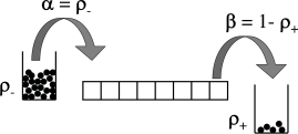
Figure 10: Incorporating $\alpha$ and $\beta$ through two reservoirs with appropriate densities.

In this approach, one imagines that the left and right ends of the system are connected to two reservoirs with the appropriate number densities $\rho_{-}$ and $\rho_{+}$ of particles (ribosomes) so that, assuming the same jumping rates as in the bulk, the rates $\alpha$ and $\beta$ are incorporated into the model (see fig.10).

The extrema principle then relates the flux ${\cal J}$ in the open system to the flux $J(\rho)$ for the corresponding closed system (i.e., the system with periodic boundary conditions) with the same dynamics. In the limit $L\to{}\infty$ popkov2 , the extrema principle states that

$${\cal J}=\left\{\begin{array}[]{ccc}max~{}J(\rho)&{\rm if}~{}\rho_{-}>\rho>\rho_{+}\\ min~{}J(\rho)&{\rm if}~{}\rho_{-}<\rho<\rho_{+}\end{array}\right.$$ (29)

In the present context of our model the expression (17) for $J(\rho)$ exhibits a single maximum at $\rho=\rho^{*}$ where $\rho^{*}$ is given by the equation (19). Moreover, we take $\rho_{+}=0$, i.e., $\beta=1$, because we assume that the ribosome is released from the mRNA as soon as it reaches the stop codon; this is justified by the fact that, normally, termination is not the rate limiting step in the process of protein synthesis. Therefore, the extremal current hypothesis implies that in our model

$${\cal J}=max~{}J(\rho)~{}{\rm if}~{}\rho_{-}>\rho^{*}$$ (30)

All the results derived in this section exploiting this extremum principle are approximate because the expression (17), which we use for the expression of $J(\rho)$, has been derived in the mean-field approximation. Next, following arguments similar to those followed in all earlier applications of this extremum principle, we now derive the appropriate expressions for $\rho_{-}$.

Consider a closed system with $L$ sites. Given that a sequence of ${\ell}$ successive sites are empty, the total number of ways in which $N$ ribosomes can be distributed over the remaining $L-{\ell}$ sites is simply $Z(L-{\ell},N,{\ell})$. Of these, $Z(L-2{\ell},N-1,{\ell})$ configuations have a ribosome in the adjacent ${\ell}$ sites to the left of these empty ${\ell}$ sites. Let us use the symbol ${\cal P}({\underbrace{11...1}_{\ell}}|{\underbrace{\underline{00...0}}_{\ell}})$ for the conditional probability that, given a sequence of ${\ell}$ successive empty sites, there will be a ribosome in the adjacent ${\ell}$ sites to its left. Then, from the above considerations,

$${\cal P}({\underbrace{11...1}_{\ell}}|{\underbrace{\underline{00...0}}_{\ell}})=\frac{Z(L-2{\ell},N-1,{\ell})}{Z(L-{\ell},N,{\ell})}=\frac{N}{L-{\ell}+N-N{\ell}}.$$ (31)

In terms of the number density $\rho$, this probability can expressed as

$${\cal P}({\underbrace{11...1}_{\ell}}|{\underbrace{\underline{00...0}}_{\ell}})=\frac{\rho}{\rho{}+1-\frac{{\ell}}{L}-\rho{}{\ell}}.$$ (32)

Moreover, solving the equations (20-26) we find

$$P_{5}=\frac{1}{1+\Omega_{h2}}$$ (33)

Therefore, if $P^{jump}$ is the probability that, given a sequence of ${\ell}$ successive empty sites, a ribosome will hop onto it in the next time step, we have

$$P^{jump} = {\cal P}({\underbrace{11...1}_{\ell}}|{\underbrace{\underline{00...0}}_{\ell}})\times{}P_{5}\times{}\omega_{h2}(\Delta t)$$ (34)

where ${\cal P}({\underbrace{11...1}_{\ell}}|{\underbrace{\underline{00...0}}_{\ell}})$ and $P_{5}$ are given by (32) and (33), respectively.

Now, going back to the open system, $\rho_{-}$ is the solution of the equation $\alpha{}=P^{jump}$ and, hence, we get

$$\rho_{-}=\frac{\alpha{}(1-\frac{{\ell}}{L})(1+\Omega_{h2})}{P_{\omega_{h}}-\alpha{}(1+\Omega_{h2})(1-{\ell})}$$ (35)

where $P_{\omega_{h}}$ is the probability of hydrolysis in time $\Delta{}t$. In the special case $k_{eff}\rightarrow\infty$ while $\omega_{h2}=q$ remains finite and non-zero, i.e., $\Omega_{h2}\rightarrow 0$, $\rho_{-}\rightarrow\frac{\alpha}{1+({\ell}-1)\alpha}$, which is identical to the expression derived earlier by Lakatos and Chou lakatos03 for this special case.

Figure 11: Phase diagram in $\alpha{}-P_{\omega_{a}}$ plane. $P_{\omega_{a}}$ is the probability of attachment of a tRNA in time $\Delta{}t=0.001~{}s$, and is related to $\omega_{a}$ by equation (38). This diagram has been plotted for $\omega_{h1}=\omega_{h2}=\omega_{h}=10~{}sec^{-1}$.

Figure 12: Phase diagram in $P_{\omega_{h}}-P_{\omega_{a}}$ plane. $P_{\omega_{h}}$ is the probability of hydrolysis in time $\Delta{}t=0.001~{}s$, and is related to $\omega_{h}$ by equation (38).

Thus, the boundaries between various phases have been obtained by solving the equation

$$\rho_{-}(\alpha{},\omega_{a},\omega_{h1},\omega_{h2})=\rho_{*}(\alpha{},\omega_{a},\omega_{h1},\omega_{h2})$$ (36)

numerically using $\rho^{*}$ and $\rho_{-}$ obtained, respectively, from equations (19) and (35); two typical phase diagrams have been plotted in in figures 11 and 12 assuming thompson ; harrington ; cross97 $\omega_{h1}=\omega_{h2}=\omega_{h}$. Each of these phase diagrams show two phases namely, a maximal current phase and another phase. In order to find out whether the latter is the low-density phase or the high-density phase, we studied the trend of variation of the density profile across the phase boundary (see fig.9). If the average density increases and, finally, saturates in the maximal current phase (as observed in the inset of fig.9(a)) while the current reaches its maximum value, we identify it with the transition from the low-density phase to the maximal current phase (as in fig.11). On the other hand, gradual decrease of the average density and its eventual saturation (as observed in the inset of fig.9(b)), while the current approaches its maximum value, indicates a transition from the high-density phase to the maximal current phase (as in fig.12).

Although the extremum current hypothesis popkov2 is believed to be exact, at least in the limit $L\rightarrow\infty$, our results on the phase boundaries are approximate because we have used the mean-field estimates (19) and (35) for $\rho^{*}$ and $\rho_{-}$, respectively, in equation (36).

VII Summary and conclusion

TASEP is the simplest model of systems of interacting “self-propelled” particles. Interestingly, the TASEP itself was developed originally macdonald68 to describe traffic-like collective movement of ribosomes on an mRNA strand. The physical properties of the TASEP and similar driven-diffusive lattice gas models have been investigated extensively in the recent years using the techniques of non-equilibrium statistical mechanics sz ; schuetz . Success of TASEP-like models in vehicular traffic css has not only led to the recent modelling of molecular motor traffic by suitable extensions of TASEP polrev ; tgf06 ; physica ; lipo3 ; frey3 ; santen ; popkov1 , but has also revived interest in ribosome traffic macdonald68 ; macdonald69 ; lakatos03 ; shaw03 ; shaw04a ; shaw04b ; chou03 ; chou04 .

In reality, a ribosome is not just a “particle” but one of the most complex natural nanomotors spirinbook . An underlying implicit assumption of the TASEP type models of ribosome traffic is that the numerical value of the hopping rate $q$ is determined by the main rate-limiting step in the mechano-chemical cycle of a ribosome. In contrast, in this paper we have developed a model of ribosome traffic during protein synthesis by explicitly incorporating all the major steps in the mechano-chemical cycle of each ribosome, in addition to the mutual exclusion of the ribosomes arising from their steric interactions. Thus, our work can be viewed as an interesting biologically motivated extension of TASEP to an exclusion process for extended particles with “internal states”. Exclusion processes with “internal states” have begun receiving attention in very recent literature reichenbach ; tabatabei .

We have calculated, both analytically and numerically, the flux of the ribosomes, which is directly related to the rate of protein synthesis. We have investigated how the rate of protein synthesis is affected by the variation of the rate constants for the various steps of the mechano-chemical cycle of individual ribosomes. We have demonstrated that, with the increase of the numerical value of a rate constant, the current eventually saturates when the corresponding step of the mechano-chemical cycle is no longer rate limiting.

We have also calculated the average density profiles of the ribosomes on the mRNA track in all the dynamical phases of the system. Using a few real mRNA sequences for E-coli, we have demonstrated that, because of the sequence inhomogeneity, the rate of protein synthesis from real mRNA templates is slower than that from a hypothetical homogeneous template. Besides, we have calculated the flux in real time (unlike arbitrary units used in most of the earlier works). Our theoretical estimates for the rates of protein synthesis are in good agreement with the corresponding experimental data.

Our work also elucidates the nature of boundary-induced non-equilibrium phase transitions in a biologically-motivated driven-diffusive lattice gas model schuetz . We have determined the phase boundaries on the phase diagrams for our model by using the extremum current hypothesis popkov2 . Following the traditional approach to phase diagrams of TASEP under OBC, all the earlier works on TASEP like models of ribosome traffic reported phase diagrams in the $\alpha-\beta$ plane. But, we have plotted the phase diagrams in planes spanned by experimentally accessible parameters that include the concentrations of aa-tRNA and GTP-bound elongation factors. We hope the predictions of our theoretical model will stimulate further experimental studies for more accurate quantitative data.

Acknowledgements: One of the authors (DC) thanks Stephan Grill, Frank Jülicher, Anatoly Kolomeisky, Alex Mogilner, Katsuhiro Nishinari and Gunter Schütz for comments on an earlier version of the manuscript and/or for drawing attention to some earlier relevant works. This work has been supported (through DC) by Council of Scientific and Industrial Research (CSIR), government of India.

Appendix A: Rate constant versus probability

Consider a chemical reaction: A$\longrightarrow$B, with a rate constant $k$. Thus,

$$\frac{d[B]}{dt}=k[A]=-\frac{d[A]}{dt}$$ (37)

Solving (37) gives

$$\frac{[A]_{\circ}-[A]}{[A]_{\circ}}=1-e^{-k\Delta{}t}$$ (38)

where [A]_∘ is the concentration of A at $t=0$. The left hand side of (38) gives the fraction of A molecules reacted in time $\Delta{}t$, and is thus the probability that a single molecule of A will be transformed into B, in time $\Delta{}t$. If this time interval $\Delta{}t$ is very small, we can expand the right hand side of equation (38). Differentiation of this with restect to time gives the probability of transition per unit time:

$$\omega_{A\rightarrow{}B}=\frac{\partial{}}{\partial{}t}\lim_{t\rightarrow{}0}(1-e^{-kt})=k$$ (39)

If $P_{A}$ is the probability of finding the molecule in state A, then the final master equation, according to (39) is

$$\frac{\partial{}P_{A}}{\partial{}t}=-\omega_{A\rightarrow{}B}P_{A}$$ (40)

Appendix B: Results in the special case ${\ell}=1$

Consider the special case ${\ell}=1$ of our model of ribosome traffic (with 5 “internal” states for each ribosome) on a mRNA of $L$ codons. This model is not equivalent to the TASEP-like model of Lakatos et al.laka05 where particles (without internal states) hop on a lattice of $5L$ sites with spatially periodic hopping rates. Under periodic boundary conditions, the factor $Q(\underline{i}|i+{\ell})$ in equations (4) and (8) reduce to the simpler form $Q(\underline{i}|i+1)=1-P(i+1)$. Thus, for ${\ell}=1$, in the steady-state with PBC,

$$P_{5}=\frac{P}{1+\Omega_{h2}(1-P)}$$ (41)

and, hence,

$$J=\omega_{h2}P_{5}(1-P)=\frac{\omega_{h2}\rho(1-\rho)}{1+\Omega_{h2}(1-\rho)}$$ (42)

In the special case $k_{eff}\rightarrow\infty$, where $\omega_{h2}=q$ is non-zero and finite, $\Omega_{h2}\rightarrow 0$; in that case the expression (42) reduces to the corresponding formula (2) for TASEP.

References

- (1) A. S. Spirin, Ribosomes, (Springer, 2000).
- (2) A.S. Spirin, FEBS Lett. 514, 2 (2002).
- (3) J. Frank and C.M.T. Spahn, Rep. Prog. Phys. 69, 1383 (2006).
- (4) R. A. Cross, Nature 385, 18 (1997).
- (5) T.L. Hill. Proc. Natl. Acad. Sci. 64, 267 (1969).
- (6) D. Chowdhury, L. Santen and A. Schadschneider, Phys. Rep. 329, 199 (2000).
- (7) D. Chowdhury, A. Schadschneider and K. Nishinari, Phys. of Life Rev. 2, 318 (2005).
- (8) A. Schadschneider, T. Pöschel, R. Kühne, M. Schreckenberg and D.E. Wolf, (eds.) Proc. of the international conference Traffic and Granular Flow ’05, (Springer, 2006).
- (9) See the issue 1 of vol.372 of Physica A (guest eds. D. Chowdhury, A. Dutta and B.K. Chakrabarti) (2006) for the close similarities and crucial differences between biological traffic and vehicular traffic.
- (10) C. MacDonald, J. Gibbs and A. Pipkin, Biopolymers, 6, 1 (1968).
- (11) C. MacDonald and J. Gibbs, Biopolymers, 7, 707 (1969).
- (12) G. Lakatos and T. Chou, J. Phys. A 36, 2027 (2003).
- (13) L.B. Shaw, R.K.P. Zia and K.H. Lee, Phys. Rev. E 68, 021910 (2003).
- (14) L.B. Shaw, J.P. Sethna and K.H. Lee, Phys. Rev. E 70, 021901 (2004).
- (15) L.B. Shaw, A.B. Kolomeisky and K.H. Lee, J. Phys. A 37, 2105 (2004).
- (16) T. Chou, Biophys. J., 85, 755 (2003).
- (17) T. Chou and G. Lakatos, Phys. Rev. Lett. 93, 198101 (2004).
- (18) J.J. Dong, B. Schmittmann and R.K.P. Zia, arXiv: q-bio.QM/0606043 (2006).
- (19) K. Nishinari, Y. Okada, A. Schadschneider and D. Chowdhury, Phys. Rev. Lett. 95, 118101 (2005).
- (20) Y. Kafri, D.K. Lubensky and D. R. Nelson, Biophys. J. 86, 3373 (2004).
- (21) Y. Kafri and D.R. Nelson, J. Phys. Cond. Matt. 17, S3871 (2005).
- (22) F. Jülicher, A. Ajdari and J. Prost, Rev. Mod. Phys. 69, 1269 (1997).
- (23) P. Reimann, Phys. Rep.361, 57 (2002).
- (24) J. Howard, Curr. Biol. (2006).
- (25) S. Varenne, J. Buc, R. Lloubes and C. Lazdunski, J. Mol. Biol. 180, 549 (1984).
- (26) S. Schilling-Bartetzko, A. Bartetzko and K.H. Nierhaus, J. Biol. Chem. 267, 4703 (1992).
- (27) G. M. Schütz, Phase Transitions and Critical Phenomena, vol. 19 (Acad. Press, 2001).
- (28) B. Schmittmann and R.K.P. Zia, in: Phase Transition and Critical Phenomena, Vol. 17, eds. C. Domb and J. L. Lebowitz (Academic Press, 1995).
- (29) J. Hiernaux, Biophys. Chem. 2, 70 (1974).
- (30) R. Gordon, J. Theor. Biol. 22, 515 (1969).
- (31) G. Vassert, J.E. Dumont and F. R. L. Canbtraine, Biochim. Biophys. Acta, 247, 471 (1971).
- (32) G. von Heijne, L. Nilsson and C. Blomberg, Eur. J. Biochem. 92, 397 (1978).
- (33) J.E. Bergmann and H.F. Lodish, J. Biol. Chem. 254, 11927 (1979).
- (34) C. B. Harley, J. W. Pollard, C. P. Stanners and S. Goldstein, J. Biol. Chem. 256, 10786 (1981).
- (35) M.A. Gilchrist and A. Wagner, J. Theor. Biol. 239, 417 (2006).
- (36) H. F. Lodish, Nature 251, 385 (1974).
- (37) A. A. Ferreira and F. C. Alcaraz, Phys. Rev. 65, 052102 (2002).
- (38) G. Schönherr and G. M. Schütz, J. Phys. A 37, 8215 (2004).
- (39) G. iSchönherr, Phys. Rev. E 71, 026122 (2005).
- (40) R.C. Thompson, D.B. Dix and J.F. Eccleston, J. Biol. Chem. 255, 11088 (1980).
- (41) K.M. Harrington, I.A. nazarenko, D.B. Dix, R.C. Thompson and O.C. Uhlenbeck, Biochem. 32, 7617 (1993).
- (42) S.G.E. Andersson and C.G. Kurland, Microbiol. Rev. 54, 198 (1990).
- (43) S. Zhang, E. Goldman and G. Zubay, J. Theor. Biol. 170, 339 (1994).
- (44) J. Solomovici, T. Lesnik and C. Reiss, J. Theor. Biol. 185, 511 (1997).
- (45) S.A. Janowsky and J.L. lebowitz, Phys. Rev. A 45, 618 (1992).
- (46) G. Schütz, J. Stat. Phys. 71, 471 (1993).
- (47) G. Tripathi and M. Barma, Phys. Rev. Lett. 78, 3039 (1997); Phys. Rev. E 58, 1911 (1998).
- (48) S. Goldstein and E.R. Speer, Phys. Rev. E 58, 4226 (1998).
- (49) K. M. Kolwankar and A. Punnoose, Phys. Rev. E 61, 2453 (2000).
- (50) R. J. Harris and R.B. Stinchcombe, Phys. Rev. E 70, 016108 (2004).
- (51) C. Enaud and B. Derrida, Europhys. Lett. 66, 83 (2004).
- (52) R. Juhasz, L. Santen and F. Igloi, Phys. Rev. Lett. 94, 010601 (2005).
- (53) M. Barma, in ref.physica .
- (54) T. Harms and R. Lipowsky, Phys. Rev. Lett. 79, 2895 (1997).
- (55) F. Marchesoni, Phys. Rev. E 56, 2492 (1997).
- (56) M.N. Popescu, C.M. Arizmendi, A.L. Salas-Brito and F. Family, Phys. Rev. Lett. 85, 3321 (2000).
- (57) Y. Jia, S.N. Yu and J.R. Li, Phys. Rev. E 63, 052101 (2001).
- (58) L. Bai, A. Shundrovsky and M.D. Wang, J. Mol. Biol. 344, 335 (2004).
- (59) V.R. Tadigotla, D.O. Maoileidigh, A.M. Sengupta, V. Epshtein, R.H. Ebright, E. Nudler and A.E. Ruckenstein, Proc. Nat. Acad. Sci. USA, 103, 4439 (2006).
- (60) see http://www.genome.wisc.edu/sequencing/k12.htm
- (61) J. Krug, Phys. Rev. Lett. 67, 1882 (1991).
- (62) V. Popkov and G. Schütz, Europhys. Lett. 48, 257 (1999).
- (63) J. Hager, J. Krug, V. Popkov and G. Schütz, Phys. Rev. E 63, 056110 (2001).
- (64) J. Hager, Phys. Rev. E 63, 067103 (2001).
- (65) R. Lipowsky, Y. Chai, S. Klumpp, S. Liepelt and M. J.I. Müller, Physica A (2006) in press and references therein.
- (66) E. Frey, A. Parmeggiani and T. Franosch, Genome Inf. 15, 46 (2004) and references therein.
- (67) M.R. Evans, R. Juhasz and L. Santen, Phys. Rev. E 68, 026117 (2003).
- (68) V. Popkov, A. Rakos, R.D. Williams, A.B. Kolomeisky and G.M. Schütz, Phys. Rev. E 67, 066117 (2003).
- (69) T. Reichenbach, T. Franosch and E. Frey, Phys. Rev. Lett. 97, 050603 (2006).
- (70) F. Tabatabaei and G. M. Schütz, cond-mat/0608147 (2006).
- (71) G. Lakatos, T. Chou and A. Kolomeisky, Phys. Rev. E 71, 011103 (2005).