Anomalous fluctuations in Minority Games and related multi-agent models of financial markets

Abstract

We review the recent approaches to modelling financial markets based on multi-agent systems. After a brief summary of the basic stylised facts observed in real-market time-series we discuss some simple agent-based systems which are currently used to model financial markets. One of the most prominent examples is here the Minority Game (MG), which we address in some more detail. After a brief discussion of its basic setup and general phenomenology we summarise the main findings of the statistical mechanics analysis and discuss the emergence of stylised facts in extensions of the MG near their phase transitions between efficient and predictable regimes. We then turn towards more realistic variants which comprise heterogeneous populations of agents, with different memory capabilities, different inclinations to trade and varying expectations on the future evolution of the market. Finally we give a short outlook on potential future work in this area.

1 Introduction

The modelling of financial markets and other social systems by means of individual-based simulations has attracted a significant amount of attention in recent years, both in the economics and socio-economics community, as well as among statistical physicists [4, 37, 55, 18, 24, 46, 58]. The range of phenomena to which this approach is applied is broad, and includes not only the modelling of traders in financial markets, but also opinion formation and decision dynamics, epidemic spreading, the behaviour of crowds and pedestrians, as well as vehicular traffic and co-operative behaviour in animal swarms [41, 42, 72, 7, 6]. The term ‘individual’ in individual-based approaches to the modelling of such systems may here stand for traders in a financial market, cars on a highway or companies in an economic network. While practitioners often make use of sophisticated models with a variety of different types of agents, statistical physicists have become interested in minimalist models of such phenomena, which ideally allow for analytical solutions. While the detail and complexity of more realistic models often impedes analytical approaches, the reduced models considered by physicists are often tractable with methods from statistical physics, and their behaviour can be characterised analytically for example by exact or approximative calculation of their phase diagrams. Furthermore the restriction to minimalist models allows one to focus on the parameters and features of the model which are truly responsible for its behaviour (e.g. by systematic adding or removal of individual features), whereas the underlying mechanisms may be obscured and thus harder to detect in more sophisticated and detailed models. Apart from the methodology, concepts of physics often allow one to shed light on phenomena in adjacent fields and to address them from novel viewpoints. The concepts of self-organised criticality [6] or replica symmetry breaking and the corresponding rugged landscape picture of spin glass physics may here serve as examples [67]. Agent-based models and models from statistical physics share common features in that in both cases one is interested in complex co-operative behaviour on a macroscopic scale emerging from relatively simple interactions at the microscopic level, i.e. between the interacting agents. One may thus expect that techniques and methods developed originally in the context of physics may be successfully employed in other disciplines as well in order to study complex many-agent systems and their emergent collective phenomena.

This review focuses on some such approaches in the context of the modelling of financial markets by agent-based trading models. Although the statistical physics analysis is limited to minimalist models, several such model systems have been seen to show remarkably complex behaviour, including phase transitions, non-trivial co-operation and global adaptation [18, 24, 46, 58]. From the point of view of the description of real-world phenomena they also display what is referred to as ‘stylised facts’ in the economics literature, namely anomalous non-Gaussian behaviour and fluctuations in their global observables, similar to statistical features seen in real market data. This positions the agent-based models considered by statistical physicists right at the boundary between being analytically solvable and at the same time sufficiently realistic, and constitutes some of the appeal of such models.

The objective of this chapter is to review some of the developments in the study of agent-based models, stressing the emergence of anomalous behaviour. While some, potentially non-representative focus is given to Minority Game market models and the authors’ own work, we also present a brief discussion of some other related agent-based models.

2 Overview and stylised facts in financial markets

2.1 Introduction

‘Stylised facts’ in the context of finance is a term used by theoretical economists and by practitioners to summarise statistical features of time series generated by financial markets. Most notably financial markets generate non-Gaussian time series with power-law characteristics, long-range correlations in time, scaling behaviour and anomalous fluctuations [58, 11]. Non-Gaussian behaviour is indeed found in many different contexts, already more than 100 years ago, Vilfredo Pareto [66] pointed out that in numerous countries and at various points in time the wealth distribution follows a power-law, i.e. $N\sim w^{-\alpha}$, where $N$ is the number of people having wealth greater than $w$. Over the past decades similar power-law behaviour has been detected in numerous other phenomena, ranging from financial time series, to sand piles, the distribution of word frequency in texts, citations of scientific papers, hits on web pages, firm sizes, populations of cities so forth [6, 64].

Anomalous, non-Gaussian fluctuations are not only observed in the above systems, apparently unrelated to physics, but also in systems of condensed matter physics, and in models of statistical mechanics. Anomalous behaviour is here found in a variety of contexts, from magnetic materials, over solutions of polymers, gels, glasses, fluid- and superfluid helium, water at its boiling point, and even in experiments of elementary particle physics and in cosmology [47, 76]. The common feature of these systems is that they display phase transitions, i.e. depending on external control parameters (such as temperature or pressure) the behaviour of one given system can be of different types. Not only do the characteristics of these systems change drastically at their transition points, but thermal fluctuations attain non-Gaussian features, very similar to those observed in unphysical systems mentioned above. Close to their critical points systems of condensed matter physics display long-range correlations, with an algebraic as opposed to an exponential decay of spatial and temporal correlations, leading to large-scale collective behaviour, ergodicity breaking and other so-called ‘anomalous’ characteristics. Power-law correlation functions are here a reflection of scale-free behaviour of the system, i.e. of fractal properties and self-similarity. This invariance under re-scaling of units has led to the development of powerful methods of statistical physics, most notably of renormalisation group, which allow to address critical phenomena efficiently [47, 76, 13].

2.2 Anomalous fluctuations in financial markets

Power-law statistics and non-Gaussian behaviour have been detected in a variety of different markets, and are mostly independent of the specific trading rules or external circumstances at the given market place [58]. For example, if we denote the price of an asset or an index by $X(t)$, then the log-return at time scale $\Delta_{t}$ is defined as $r_{t}=\ln\left(X(t)/X(t-\Delta_{t})\right)$. Empirical studies show that the distribution of log-returns has power-law tails with exponents between $3$ and $5$ [39]. Another interesting feature which is observed in financial markets is the so-called volatility clustering: while the correlation of returns decays relatively quickly in time, the correlation of the absolute log-returns, defined as $C_{|r|}(\tau)=\left\langle|r(t+\tau)||r(t)|\right\rangle$, follows a long-range power-law distribution with an exponent ranging from $0.1$ to $0.3$ [56, 54]. Non-Gaussian distributions are also observed when looking at the trading volume or the number of trades per time. We illustrate these observations in Fig. 1, where a financial time-series with a characteristic non-Gaussian behaviour is shown, along with its algebraically decaying return distribution.

Given the abundance of financial data physicists have become involved in the analysis of time series of markets, as well as in research aiming to model the processes generating these data. This field at the borderline of statistical physics, econometrics and financial mathematics is now known as econophysics [14]. The attempts to model financial markets here roughly fall into two classes, phenomenological models and agent-based approaches. In the next section we will briefly discuss both, and then concentrate on the latter agent-based approach, as mentioned in the introduction. We will here mostly focus on qualitative aspects, and will not enter mathematical details of the various models. For a recent textbook on mathematical aspects of MGs and related models see also [24].

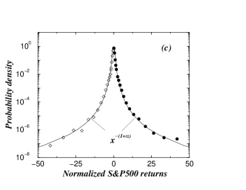
Figure 1: Left: Sequence of 10 min returns of the S&P 500 index (top), 1 month returns (middle), and a realisation of a Gaussian random walk for comparison. Right: Linear-log plots of the probability distribution for the normalized S&P500 returns. The solid lines are power-law fits with exponents $1+\alpha\approx 4$. Figures taken from [39].

3 The agent-based approach

3.1 Random walks and other phenomenological models

Many approaches to anomalous statistical properties of financial data are based on direct modelling of stock market indices as stochastic processes. Such models do not deal with the market on a microscopic level, i.e. with individual agents, but with aggregate quantities only, such as the stock market indices, their return statistics and fluctuations on a macroscopic level. The very first of such theories dates back to Bachelier’s ‘Théorie de la Spéculation’ from 1900 [5] and describes the stochastic evolution of market indices as simple Gaussian random walks. While it is now well established that market data is fundamentally non-Gaussian, Bachelier’s theory of financial markets as log-normal random walks still forms the basis of many phenomenological approaches to finance. Most notably, the Black-Scholes theory [12] commonly used for the pricing of financial derivatives relies entirely on Gaussian assumptions, and hence on Bachelier’s approach.

More realistic approaches to finance with stochastic processes are of course no longer based on purely Gaussian processes, but use Lévy flights and related processes to model the temporal evolution of financial indicators [11]. Many different classes of stochastic processes have here been used, partially relying on the fact that multiplicative as opposed to additive Gaussian noise directly leads to power-law behaviour.

3.2 Agent-based models

While phenomenological models can describe many features observed in real markets, they are at least to some extent not fully satisfactory in that they do not allow for a derivation of global quantities from the most basic level of description, namely the direct interaction between agents. These phenomenological and agent-based approaches are, to some degree, analogous to the description of physical phenomena through thermodynamics and statistical physics respectively. While the laws of thermodynamics, such as for example the phenomenological equation describing an ideal gas, find their justification mostly in the purely empirical observation, only a direct kinetic theory allows for a description on the level of individual molecules. During 19th century such a kinetic theory was being developed, starting from Newton’s laws and using probabilistic arguments, and results from thermodynamics were re-derived from first principles, marking the beginning of statistical mechanics.

One can think of phenomenological models of financial markets as the analogue of the description of physical phenomena on the level of thermodynamics. Empirical laws like the ideal gas equation here correspond to the stylised facts empirically found in time series of financial markets. The aim of phenomenological models is thus, in essence, to devise and study stochastic processes for macroscopic observables, without considering the detailed microscopic interaction which bring about the global phenomena.

The counterpart of statistical mechanics would then be given by models which start from the level of the individual interacting particles of a financial market, i.e. the traders. While in physics particles can be considered the basic elements, in markets this role is played by financial agents. The objective of statistical mechanics approaches to financial markets is thus to study the interactions between individual agents, and to derive equations describing global quantities from these microscopic rules of engagement. Naturally the analogy between particles and agents is limited, for example because agents are intelligent and particles are of course not. However, concepts and techniques from physics can be transferred to the study of agent-based systems, which mathematically turn out to be surprisingly similar to models of statistical physics.

The remainder of this review will focus on agent-based models. These allow one to address fundamental questions for example as to where anomalous fluctuations may actually come from on the level of the behaviour of the agents. Agent-based models of financial markets have attracted substantial attraction, both in the economics and in the physics communities. They easily accessible by computer simulations, so that effects of changes in the rules of engagement of the agents, the ecology of the model-market or variations in external control parameters are readily examined. The role of physicists has here mostly been to devise simple minimalist models of financial markets, which are also accessible analytically and conceptually by tools of statistical mechanics.

4 Minority Games and related models

4.1 Introduction

Neoclassical economics usually assumes that agents have perfect, logic and deductive rationality, as well as full information about the market [78, 62, 71]. This implies, among other things, that they are homogeneous and that they act always in the best possible way. Common sense suggests that this view is quite far from reality and for different reasons people are neither completely rational nor deductive and homogeneous. Starting from this observation, leading economist Brian Arthur introduced a very simple model, now known as the ‘El Farol bar problem’, to illustrate bounded rationality and inductive reasoning. In Arthur’s model agents have only limited information and modes of reacting to it at hand, and learn inductively from past experience. The mathematical abstraction of this model resulted in the Minority Game (MG) [19], which now also serves as one of the most popular toy models for financial markets.

Despite its simplicity, the MG exhibits a very rich behaviour, with phases in which the resulting model-market behaves fully inefficiently and others in which the time-series generated by the market still has some information-content, leading to an effective predictability. As a function of the model parameters, the agents can either co-operate successfully and achieve total gains higher than if they were to play at random, or in other regimes fail to adapt successfully, resulting in high losses.

In its original formulation the statistics of the MG are mostly Gaussian (if large populations of agents are considered), and there are no signs of volatility clustering and other stylised facts in the time-series generated by the most basic MGs. Small modifications, however, can produce the fat tailed distributions similar to those observed in financial markets. Apart from the appeal of the MG as a market model, it has also attracted a significant interest as a model of statistical mechanics, and the methods of theoretical spin glass physics have been seen to provide insight into its phase behaviour, and have revealed new types of global co-operation, complexity and phase transitions, previously unknown in models of disordered systems theory [18, 24].

4.2 Definition of the MG model

The MG is a mathematical abstraction of the El-Farol bar problem. In the latter a group of say $100$ agents have to decide whether or not to attend a bar at a given night every week. In general people will only enjoy being at the bar if not more than say $60$ people attend that night, as otherwise the bar will be too crowded. Every agent has to decide independently every week whether to go or not, and has to make that decision on the basis of the time-series of previous attendances. El-Farol agents in Arthur’s model are agents of bounded rationality who learn inductively. Each of them holds a set of predictors, mapping the past attendances onto a future (predicted) one, and based on these idiosyncratic predictions the individual agents decide on whether or not to attend the bar.

The basic MG model describes this systems as a population of $N$ agents (with $N$ an odd integer), in which every player $i$ has to take a binary decision $b_{i}(t)\in\{-1,1\}$ at every time-step $t$. The total attendance is then computed as

$$A(t)=\sum_{i=1}^{N}b_{i}(t),$$ (1)

and agents who take the minority decision are rewarded after each round, that is if the number of agents playing $1$ is higher than the number of those playing $-1$ then all $-1$-players are rewarded and vice versa. In order to take their decisions agents are each equipped with a pool of $S$ so-called ‘strategy tables’. Assuming that agents can remember the correct minority decisions of the last $M$ rounds, that is they can resolve $P=2^{M}$ different histories of the game, a strategy $a_{is}$ provides a map from all possible $M$-step histories onto the binary set $\{-1,1\}$, i. e.

$$a_{is}:\{1,2...,P\}\rightarrow\{-1,1\}.$$ (2)

In order to take their trading decisions agents follow an inductive learning dynamics. They are limited to the strategies assigned to them at the beginning of the game, reflecting the boundedness of their rationality. These strategy assignments are typically generated at random, and result in a heterogeneous population of traders. At each time step each agent has to choose which of his strategy tables to use, and the agents do so by learning from past experience. A score $U_{i,s}$ (utility function in terms of economics) is assigned to each strategy table and updated at each step of the game as follows:

$$U_{i,s}(t+1)=U_{i,s}(t)-a_{i,s}^{\mu(t)}A(t).$$ (3)

Here $a_{i,s}^{\mu(t)}$ is the action prescribed by the strategy $s$ of agent $i$ when the history $\mu(t)$ occurs. The term $-a_{i,s}^{\mu(t)}A(t)$ reflects the minority rule: when $a_{i,s}^{\mu(t)}$ and $A(t)$ have opposite signs, i.e. if the strategy predicted the correct minority decision, then the strategy score $U_{i,s}$ is increased. If $a_{i,s}^{\mu(t)}A(t)>0$, the score is decreased. Each agent then at each time step uses the strategy table in his pool of strategies with the highest score, i.e. the one that would have performed best so far, had this particular player always used the same strategy. In case of equal scores between some strategies, the agent chooses between those at random.

4.3 Motivation as market model and price process

The MG can be understood as a simplified emulation of a financial market. The binary decisions of the agents are interpreted as ‘buying’ versus ‘selling’, and hence the aggregate action corresponds to an ‘excess demand’ in this model market, and leads to movements of the (logarithmic) price. More precisely, if $p(t)$ is the price of the good traded on the MG-market, then $\log p(t+1)=\log p(t)+\frac{A(t)}{\lambda}$, with $A(t)$ the above aggregate action $A(t)=\sum_{i=1}^{N}b_{i}(t)$. $\lambda$ here reflects the liquidity of the market and represents a proportionality constant. Traders in the MG take their decisions based on commonly available information, which may be related to the past price history of the market under consideration or to information provided externally. The payoff structure of the MG can here be derived from expectations of the agents on future price evolution [59]. Minority game agents effectively correspond to contrarian traders who expect the price to go down in step $t+1$ if it went up in step $t$. It is straightforward to extend the model to majority game or mixed minority/majority games (in which some agents play an minority game, and others a majority game) [28, 24]. Majority game agents here represent so-called ‘trend-followers’ in a real market, their expectation is that the price movement of time step $t+1$ will be in the same direction as at time $t$, so that it is favourable to buy when the majority of players is buying, and to sell whenever the majority is selling.

4.4 Behaviour and main feature of the MG

We will now turn to a brief discussion of the main phenomenology of the MG. While it follows directly from symmetry arguments that the time average of total bid vanishes for large system sizes (i.e. $<A(t)>=0$), the fluctuations of $A(t)$ display a remarkably complex behaviour when looked at as a function of the memory capacities of the agents. It was observed in [69] that the ratio $\alpha=P/N$ is the relevant scaling parameter of the model, i.e. that $\sigma^{2}/N=\overline{<A(t)^{2}>}/N$ and other observables depend on the memory length $M=\log_{2}P$ and the system size only through the ratio $\alpha=P/N$. The variance $\sigma^{2}$ of $A(t)$, also referred to as the volatility is a measure for the efficiency of the game in terms of co-operation and global gain. The smaller $\sigma^{2}$ the smaller is the group of losing agents (i.e. the majority group), with $A(t)\approx 0$ (i.e. $\sigma^{2}\approx 0$) corresponding to a situation in which close to half of the agents take either trading decision, i.e. with roughly $N/2$ agents losing and the other $N/2$ agents winners (up to corrections to lower order in $N$). A detailed analysis shows that the global gains are in fact given by $-\sigma^{2}$, due to the inherent negative-sum character of the MG global gains are always non-positive.

The behaviour of the re-scaled volatility $\sigma^{2}/N$ as a function of $\alpha$ is depicted in Fig. 2. For large $\alpha$ one finds $\sigma^{2}/N\approx 1$ which corresponds to the so-called ‘random trading limit’. As $\alpha$ is decreased one finds a minimum of $\sigma^{2}/N$ at intermediate $\alpha$, and a large volatility $\sigma^{2}/N>1$ as $\alpha\to 0$ (for zero initial conditions). In this regime the co-operation among MG agents is worse than the random trading limit, mostly due to collective motion of whole crowds of agents taking the same trading decision (and of the corresponding anti-crowds) [46, 44, 45].

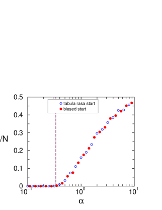
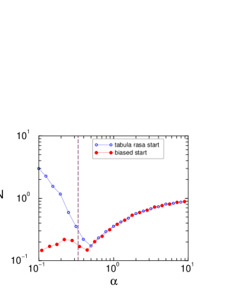
Figure 2: (Colour on-line) Left: Predictability as a function of $\alpha$ for the standard MG for tabula rasa starts (open markers) and biased initial conditions (solid markers). Right: Volatility.

Further insight can be obtained by defining the quantity

$$H=\sum_{\mu=1}^{P}\left\langle A|\mu\right\rangle^{2},$$ (4)

where the $<A|\mu>$ is the average of $A$ conditional to the occurrence of a particular history string $\mu$. $H$ is here a measure for the predictability of the system: if $<A|\mu>\neq 0$ for at least one $\mu$ then the system is predictable (in a probabilistic sense). $H=0$ thus corresponds to a fully information-efficient market, in which no exploitable information is contained in the market’s time series. If $H>0$, however, statistical predictability is present, and the market is not operating at full information efficiency.

Plotting $H/N$ as a function of $\alpha$ (see Fig. 2) one finds that the value $\alpha_{c}$ marking the minimum of $\sigma^{2}/N$ corresponds to a transition point between a predictable phase at $\alpha>\alpha_{c}$ and a fully information-efficient one at $\alpha<\alpha_{c}$.

At the same time, $\alpha_{c}$ also marks an ergodic/non-ergodic phase transition. This can be demonstrated upon plotting the volatility $\sigma^{2}/N$ as a function of $\alpha$ obtained from simulations of the MG learning dynamics started from different initial conditions. One here distinguishes so-called ‘tabula rasa’ initial conditions, for which all strategy scores are set to zero at the beginning of the game, and so-called ‘biased starts’, where some strategies receive random non-zero score valuations $U_{is}(t=0)=\pm u_{0}$ at the beginning (with $u_{0}\sim{\cal O}(1)$). A corresponding plot is shown in Fig. 2, and demonstrates that the system is insensitive to initial conditions above $\alpha_{c}$, but that the starting point becomes relevant in the information-efficient phase below the phase transition.

4.5 The statistical mechanics approach

Since its mathematical formulation in 1997 [19] the MG has attracted significant attention in the statistical physics community. In particular it has been found that the MG is accessible by the tools of the theory of disordered systems and spin-glasses [67, 32], and that its phase diagram and key observables can be computed either exactly or in good approximation by methods of equilibrium and non-equilibrium statistical mechanics. The analogy to disordered systems, which have studied in the spin-glass and neural networks communities for $30$ years, is here threefold: firstly, the random strategy assignments which are drawn at the start of the MG and through which the agents interact with each other correspond to ‘quenched disorder’ in statistical physics, that is frozen, fixed interactions between the microscopic degrees of freedom. In spin glasses the interactions are specified by the couplings between magnetic spins, in neural networks they are reflected by fixed synaptic structures governing the firing patterns of the network of neurons. Secondly, the MG displays global frustration (not everybody can win), similar to spin-glass models where not all interactions between spins can be satisfied. Thirdly, in the MG every agent interacts with everybody else (through the observation of the aggregate action $A(t)=\sum_{i}b_{i}(t)$ which is used to update strategy scores). This makes the MG a ‘mean-field’ model in the language of physics, and tools to address such systems are readily available.

We will here not enter the details of the mathematical analysis of the MG, but would only like to mention briefly that it can be addressed by both static methods such as replica techniques [67], and by dynamical approaches relying on path-integrals and dynamical generating functionals [24, 40]. We will briefly sketch the ideas of both approaches in the following two subsections.

4.5.1 Statics: replica theory

The starting point of the static replica approach to the standard MG is the function $H$ as defined above [18]. Although $H$ is not an exact Lyapunov function of the MG learning dynamics, $H$ can be seen as a ‘pseudo-Hamiltonian’, with the ergodic stationary states of the MG corresponding to extrema of $H$. If one restricts the discussion to a two-strategy MG (that is each agent $i$ holds only two strategy tables $a_{is}$ with $s=\pm 1$), then $H$ turns out to be given by

$$H=\frac{1}{\alpha N}\sum_{\mu=1}^{\alpha N}\left(\sum_{i}\{\omega_{i}^{\mu}+\xi_{i}^{\mu}m_{i}\}\right)^{2}$$ (5)

where $\xi_{i}^{\mu}=\frac{1}{2}(a_{i,1}^{\mu}-a_{i,-1}^{\mu})$ and $\omega_{i}^{\mu}=\frac{1}{2}(a_{i,1}^{\mu}+a_{i,-1}^{\mu})$. The $\{m_{i}\}$ are here soft spin variables $m_{i}\in[-1,1]$ and (up to normalisation) correspond to the relative frequencies with which each player employs each of his two strategies.

$H$ as defined above is a random function in that it depends on the $\{\xi_{i}^{\mu},\omega_{i}^{\mu}\}$, which reflect the random strategy assignments at the beginning of the game. In the language of spin-glass physics, $H$ contains quenched disorder. Information about the stationary states of the MG can then be obtained upon minimising $H$ with respect to the microscopic degrees of freedom $\{m_{i}\}$. The starting point is the partition function

$$Z=\int_{-1}^{1}dm_{1}\cdots dm_{N}\exp\left(-\beta H(m_{1},\dots,m_{N})\right)$$ (6)

where the ‘annealing temperature’ $T=1/\beta$ is taken to zero eventually to obtain the minima of $H$,

$$\mbox{min}~{}H=-\lim_{\beta\to\infty}\frac{1}{\beta}\ln Z.$$ (7)

The explicit analytical computation of the partition function for any particular assignment of the strategy vectors this an insurmountable task, due to complex interaction and global frustration. One hence restricts to an effective average $\overline{\cdots}$ over the disorder, and considers typical minima of $H$

$$\overline{\mbox{min}~{}H}=-\lim_{\beta\to 0}\frac{1}{\beta}\overline{\ln Z}.$$ (8)

The disorder-average of the logarithm of the partition function can here be obtained using a replica-approach, as it is standard in spin-glass physics. In particular one has

$$f=-\lim_{n\to 0}\lim_{\beta\to 0}\lim_{N\to\infty}\frac{1}{\beta Nn}\left(\overline{Z^{n}}-1\right)$$ (9)

for the free energy density in the thermodynamic limit. $Z^{n}$ here corresponds to an $n$-fold replicated system, the disorder-average generates an effective coupling between the different replicas.

The further mathematical steps are tedious, but straightforward, and we will not report details here [18, 24, 61], but will only mention that order parameters such as $\lim_{N\to\infty}H/N$ and $\lim_{N\to\infty}\sigma^{2}/N$ in the ergodic phase can be obtained exactly or in good approximation from this approach. The location of the phase transition at $\alpha_{c}=0.3374...$ can be identified exactly as the point at which the so-called ‘static susceptibility’ diverges, indicating the breakdown of the ergodic replica-symmetric theory.

4.5.2 Dynamics: generating functional analysis

The dynamical approach based on generating functionals deals directly with the learning dynamics of the agents, which can be formulated as follows

$$q_{i}(t+1)=q_{i}(t)-\frac{1}{N}\xi_{i}^{\mu(t)}\sum_{j}\left\{\omega_{j}^{\mu(t)}+\xi_{j}^{\mu(t)}\mbox{sgn}[q_{j}(t)]\right\},$$ (10)

if $q_{i}(t)$ denotes the score difference $q_{i}(t)=\frac{1}{2}\left(u_{i,1}(t)-u_{i,-1}(t)\right)$ of player $i$’s two strategies at time-step $t$ in a two-strategy MG (a generalisation to $S>2$ has recently been reported in [70]). Note that only this difference is relevant for the agent’s decision which of his two look-up tables to use, and that at $t$ he will choose the strategy with the higher-score, i.e. strategy table $-1$ if $q_{i}(t)<0$ and strategy table $+1$ if $q_{i}(t)>0$. This may be summarised as him playing strategy $\mbox{sgn}[q_{i}(t)]\in\{-1,1\}$ at $t$, and hence taking trading action $\omega_{i}^{\mu(t)}+\xi_{i}^{\mu(t)}\mbox{sgn}[q_{i}(t)]$ ($=a_{i,+1}^{\mu(t)}$ if $q_{i}(t)>0$ and $=a_{i,-1}^{\mu(t)}$ if $q_{i}(t)<0$).

One the defines a dynamical analogue of the partition function as the generating functional [40, 24, 25]

$$Z[\psi]=\int\left[\prod_{i,t}Dq_{i}(t)\right]\delta(\mbox{equations of motion})\exp\left(i\sum_{it}\psi_{i}(t)\mbox{sgn}[q_{i}(t)]\right),$$ (11)

where ‘equations of motion’ is an abbreviation for Eqs. (10) so that the delta-functions restrict this path integral to all trajectories of the system allowed by the update rules. $\psi_{i}(t)$ is a source term, and allows one to compute correlation functions upon differentiation with respect to the $\{\psi_{i}(t)\}$. Mathematically speaking $Z[\psi]$ is the Fourier transform of the probability measure in the space of dynamical paths corresponding to the MG update rules, and contains all relevant information on the dynamics of the system. Similarly to the replica approach the evaluation of $Z[\psi]$ is intractable for individual realisations of the disorder, but is carried out as an average over all possible strategy assignments. This leads to a set of closed, but complicated equations for the dynamical order parameters of the problem (the response and correlation functions), from which one can proceed to compute stationary order parameters such as the volatility or the predictability. We will not report these calculations here, but will only mention that both approaches, the static replica theory and the dynamical generating functional analysis, lead to identical expressions for the characteristic observables, and ultimately deliver the same value for the phase transition point $\alpha_{c}$ [24].

While there are still some mathematical subtleties to be resolved, the MG is now essentially considered to be solved as its phase diagram and stationary states can be computed exactly, and as valid and convincing approximations for the volatility are available at least in the ergodic phase. Open questions mostly relate to the behaviour in the non-ergodic phase, where the market is information-efficient ($H=0$). Up to now, no analytical solutions have been found here.

5 Anomalous fluctuations in Minority Games and other agent-based models

5.1 General remarks

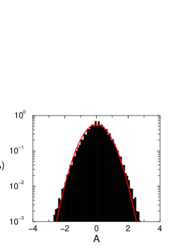
Figure 3: Return distributions of standard MG, left: symmetric phase ($\alpha\approx 0.01$), right asymmetric phase ($\alpha\approx 2$). Red line in right panel represents a fit to a Gaussian distribution.

The MG in its most simple setup does not display stylised facts, such as anomalous fluctuations or temporal correlations of the market volatility. On the contrary, return distributions are either Gaussian or of an unrealistic multi-peak shape (due to global oscillations of the system), see Fig. 3. Within the minimalist approach of statistical mechanics it is then natural to ask what features need to be added to produce more realism. It here turns out that an evolving trading volume appears to be crucial. While in the standard MG every agent trades precisely one unit at every time to make the total trading volume equal to the number $N$ of agents, two approaches have been pursued which allow for dynamically evolving trading volumes. These are referred to as grand canonical MGs (GCMG) [21, 22] and MGs with dynamically evolving capitals [16] respectively and will be detailed in the following section. GCMG here refers to MGs in which each agent is given the option to abstain at any given trading period. If they decide to trade they still trade one unit, but due to the number of active agents fluctuating in time, the total trading volume will evolve accordingly. The second approach consists in MGs with dynamically evolving capitals, that is the wealth of each agent evolves in time according to his success or otherwise in the game, and it is assumed that the amount traded by a given agent is proportional to his wealth at the time. Since the wealths change over time so does the trading volume.

We note at this stage that this tracing back of the emergence of stylised facts to a modulated total trading volume can be criticized, as liquidity effects normally also need to be taken into account in real markets. If one assumes that the total trading action $A(t)$ is related to the evolution of the (logarithmic) price via $\log p(t+1)=\log p(t)+\frac{A(t)}{\lambda}$, then the role of the liquidity $\lambda$ needs to be considered carefully. It controls the impact of the excess demand $A(t)$ on the price returns, and may well vary in time as well, i.e. $\lambda=\lambda(t)$. We will here disregard this fact, and will describe the emergence of stylised facts in GCMGs and MGs with dynamical capitals in the following section, before we then turn to a discussion of anomalous fluctuations in agent-based models different from the MG.

5.2 Anomalous fluctuations in MGs

5.2.1 Grand canonical MGs

In grand-canonical MGs agents are equipped with $S\geq 1$ ‘active’ strategies, that is strategy tables with binary entries $\{-1,1\}$ for each history, prescribing to buy or sell. Furthermore they each hold one null-strategy, i.e. a trivial strategy which prescribes to abstain for any given history-string ($a_{is}^{\mu}\equiv 0$). For each of these $S+1$ strategies they then keep score values as usual and play the one with the highest score at any time-step. An additional parameter $\varepsilon$ is here introduced, and plays the role of a disincentive for the players to be active. This is implemented by subtracting an amount $\varepsilon$ of the score of any strategy but the zero one at any time step, so that the score update rules for the ‘active’ strategies read

$$U_{is}(t+1)=U_{is}(t)-a_{is}^{\mu(t)}A^{\mu(t)}-\varepsilon.$$ (12)

The zero-strategy will always carry score zero. Thus agents trade only if the marginal payoff from trading exceeds a threshold $\varepsilon$. Modifying $\varepsilon$ thus can be understood as introducing a trading fee to the model [9].

Figure 4: Phase diagram of the grand-canonical MG. Stylised facts are observed in finite systems in a region around the efficient phase of the infinite-size model.

Since the MG by definition is a negative-sum game (i.e. the sum of all payoffs is negative), agents loose on average when trading (only a minority of players wins at every time step). Thus in the long-run all traders would stop trading in the grand-canonical setup. To maintain trading activity one usually couples the above group of ‘speculators’ (that is agents who have the option to abstain) to a background of so-called ‘producers’. The latter are endowed with only one non-zero strategy, and do not have the option not to trade, even if in the long run they lose money on the MG market. They are considered producers who make their profits from trading outside the model, and who are forced to be active on the MG market no matter what (e.g. internationally operating co-operations who need to be active in currency markets, but make their profits elsewhere).

The resulting phase diagram of the model at a fixed relative number of speculators and producers is shown in Fig. 4 in the $(\alpha,\varepsilon)$-plane. For $\varepsilon=0$ one observes the standard transition of the MG, between an unpredictable phase and a predictable one. The unpredictable phase (in which $H=0$) is marked by a red line in Fig. 4 and extends from some value $\alpha_{c}$ (which depends on the composition of the population of agents, i.e. the relative concentrations of producers and speculators) to smaller $\alpha$. Here the system is in a non-ergodic state, the so-called turbulent regime. For $\varepsilon\neq 0$ this transition is absent and the model market is predictable for all $\alpha$. Generally the predictability vanishes as $H\sim\varepsilon^{2}$ as $\varepsilon\to 0$ for $\alpha<\alpha_{c}$.

Figure 5: Return time series of a grand-canonical MG in the critical region. From [22].

The above phase diagram is obtained from the statistical mechanics theory in the thermodynamic limit $N\to\infty$, and anomalous behaviour can at most be expected for parameters corresponding to the red line in Fig. 4 in the infinite system. Simulations show, however, that anomalous fluctuations are observed in finite system in a ‘critical region’ around the critical line, as indicated by the gray area in Fig. 4. Examples of corresponding time-series are in this critical region are shown in Fig. 5. As the system size is increased this critical region shrinks, and finally reduces to the critical line of the infinite system as the number of players diverges.

5.2.2 MGs with evolving capitals

Figure 6: Return fluctuations and total wealth of the population of traders in an MG with dynamical capitals. From [16].

In MGs with dynamical capitals each agent $i$ in addition to his $S$ strategies (all different from the null strategy) holds a wealth $c_{i}(t)$ which evolves in time depending on his success or otherwise during trading. It is then assumed that he invests a constant fraction $\gamma$ of this capital $c_{i}(t)$ at time $t$. The evolution of the capital of player $i$ is then given by

$$c_{i}(t+1)=c_{i}(t)-\gamma c_{i}(t)b_{i}\frac{A(t)}{V(t)},$$ (13)

with $V(t)$ the total trading volume, $A(t)$ the excess demand at time $t$, and $b_{i}(t)$ player $i$’s trading decision at time $t$. The minus sign again reflects the minority game payoff. As in the GCMG one couples the group of speculative traders (whose volume is taken to evolve in time according to the above rule) to a group of producers, who each trade a constant volume. This model was studied in [16], and it was seen that the standard transition of the MG is preserved when introducing dynamical capitals (as illustrated in Fig. 6). At low $\alpha$ the system is in an efficient phase, which turns out to be an absorbing state of the dynamics. Above a critical value of $\alpha$ the dynamics do not approach a fixed point, and one finds $H>0$, just as in the standard MG with fixed wealth. The overall wealth of the population attains a maximum at $\alpha_{c}$ as shown in Fig. 6. We note here that results of [16] rely mostly on simulations, as an analytical solution of MGs with dynamical capitals and $S>1$ strategies per player is tedious due to the presence of fast degrees of freedom (decisions which strategy to use) as well as slow ones (the capitals), requiring an adiabatic decoupling. A theory for model with dynamical capitals and only $S=1$ strategy per player is in progress [34], and shows that the standard MG transition is present also in this simplified system.

Similar to the observations in the GCMG simulations reveal the emergence of anomalous fluctuations in finite systems in a region around $\alpha_{c}$. This is illustrated in Fig. 7, where the autocorrelation of absolute returns is shown and seen to exhibit algebraic decay, indicating long-range volatility correlations. At the same time return distributions close to the critical point are strongly non-Gaussian (see right panel of Fig. 7). While these distributions are essentially Gaussian far away from the critical point, they attain fatter and fatter tails as $\alpha_{c}$ is approached (from above), so that the kurtosis of these distributions may well be seen as measure of the distance from the critical point.

Figure 7: Left: Correlation function of absolute returns in an MG with dynamical capitals. The phase transition point is located at $\alpha_{c}\approx 0.6$ for the parameters used, volatility clustering becomes pronounced close to the transition. Right: Distribution of returns in an MG with dynamical capitals. With the parameters used one has $\alpha_{c}\approx 0.32$. Close to the transition (left) returns collapse on non-Gaussian distributions for different time-lags $dt$, far from the transition (right) a cross-over to a Gaussian occurs. Figures taken from [16].

5.3 Other market models

The MG is only one out of many market agent-based models developed in recent years, and although this topical review mostly focuses on the MG, we will provide a brief list of other models, without claiming to be exhaustive.

We will firstly discuss some close cousins of the MG, then briefly mention market models which are conceptionally different. We here partly lean on the more extensive reviews [52] and [43, 55].

While the MG is a ‘one-step’ game, i.e. a model in which all trading action takes place in a single step, this may seem incompatible with speculative market which have an intrinsic intertemporal nature: buying at a price $p(t)$ is only profitable if one is able to sell at a higher price $p(t_{1})$ where $t_{1}>t$. This lead the authors of [38, 10] as well as Andersen and Sornette [1] to use a different payoff function,

$$g_{i}(t+1)=a_{i}(t)A(t+1).$$ (14)

The model of [1] is here also known as the ‘dollar game’. Payoffs of the form of (14) imply that strategies involve two periods of time. The dynamics induced by this is characterized by different regimes in which the minority and majority nature of the interaction alternate [30]. However the majority rule prevails more often and gives rise to a phenomenon quite similar to bubble phases in real markets. See also [15] for an extension of MGs to multi-step models.

Agent based models can roughly be divided into two classes: few-strategy and many-strategy models. When they first were introduced, models of financial markets were intended to recreate the situation observed in real markets as closely as possible and for this reason they were called ‘artificial financial markets’. Initially the main purpose of these models was to carefully analyze a small number of strategies used by agents, which is why they are referred to as few-strategies models. Example of such models are those by Kirman [49] and by Frankel and Froot [31]. Concepts such as chartist and fundamentalist behaviour were first introduced in the context of agent-based simulation in these models.

In many-strategy models, on the other hand, the dynamic ecology of strategies is studied with the aim of understanding their co-evolution over time and to see what strategies will survive and which will die. The Santa Fe Artificial Stock Market (SF-ASM) [3, 50] is probably the most known example of this type of models. Its main objective is to characterise the conditions under which the market converges to an equilibrium of rational expectations. In the Genoa artificial stock market [68] randomly chosen traders place a limit buy or sell order (see also [11] for further details) according their budget limitation, and they show herding behavior similar to the one studied in the Cont-Bouchaud model [23]. We would also like to mention the Levy-Levy-Solomon model [53, 55] in which agents can switch between a risky asset and a riskless bond and do not use complicated strategies, but try to maximize a one-period utility function which implies a wealth-dependent impact of agents on prices, in contrast with the other models mentioned. Strategy switching, finally is at the centre of the model by Lux and Marchesi [57]. In this model a mixed population of noise traders (who can either be optimistic or pessimistic), and so-called fundamentalists is studied. Agents can then switch between these groups dynamically. Finally, there are of course other market models which deserve mentioning in principle, but which we can not list here due to space limitations.

With this plethora of models at hand, all or at least most of which in some regions of their respective parameter spaces reproduce market-like stylised facts it is of course legitimate to ask for a justification for this variety of models, and ultimately for a selection among them. Apart from its application as a model of a market, the MG presumably has its own right as a spin glass system and has introduced new types of complexity and phase transitions to the theory of disordered systems. Its appeal thus rests, as pointed out already above, in its position at the boundary of a realistic (within reason), though analytically solvable complex system.

6 Towards more realism: heterogeneous populations of agents

6.1 General remarks

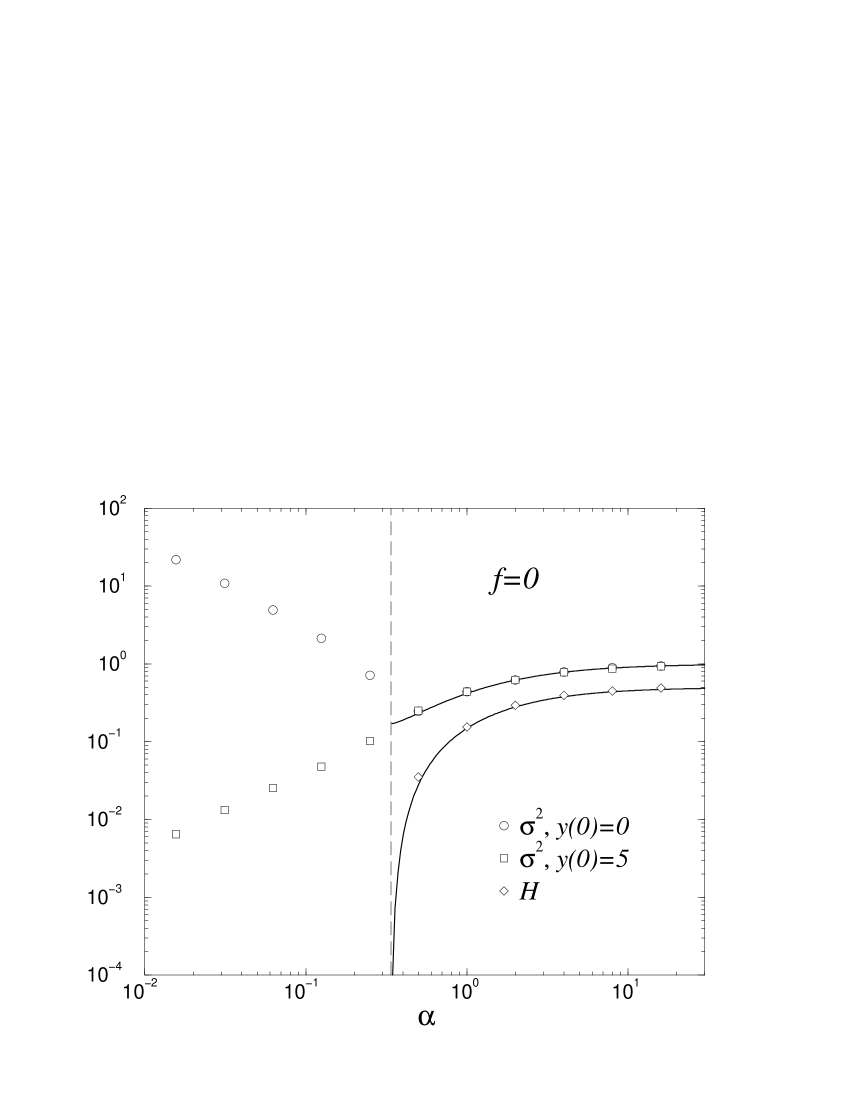
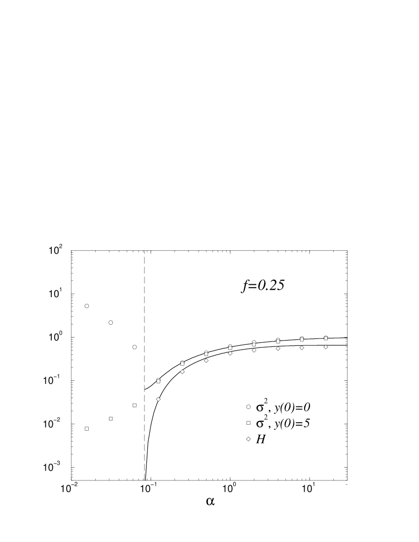
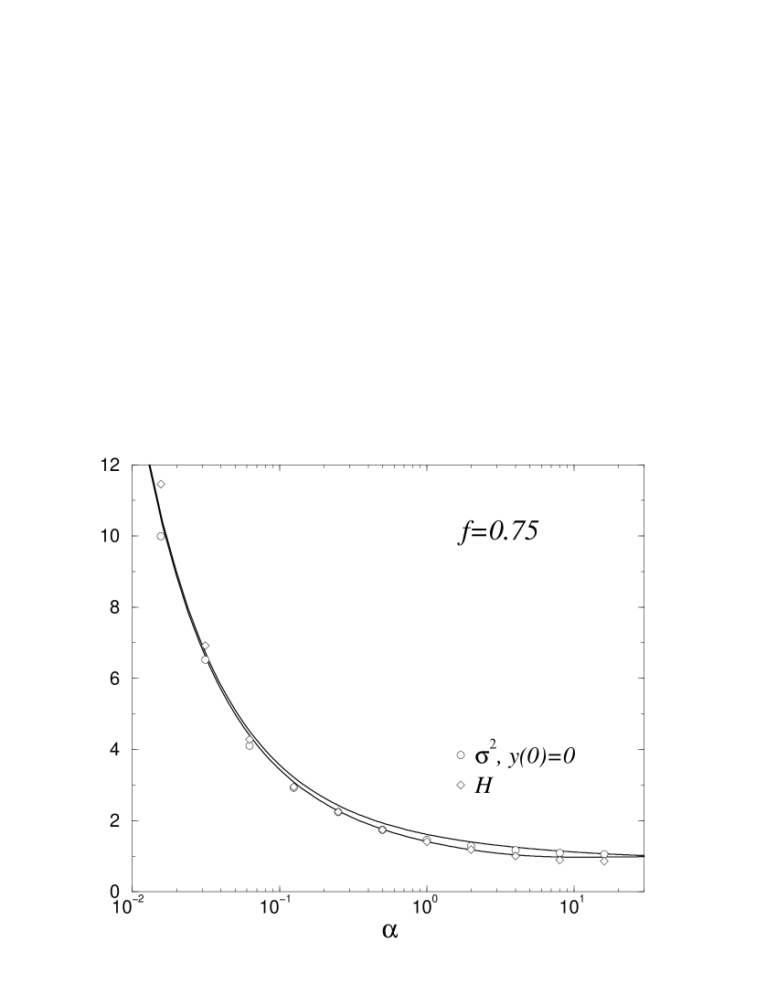
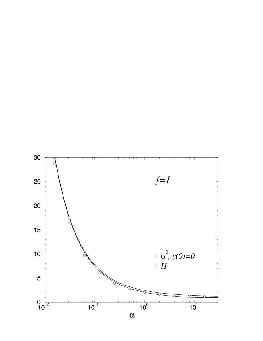
Figure 8: Behavior of $\sigma^{2}$ and $H$ vs $\alpha$ in the mixed minority/majority game for different proportions of trend-followers and contrarians. $f$ denotes the fraction of majority games players (trend-followers). From [28].

One of the main drawbacks of the MG as a market model is its simple set-up. Apart from the random assignments of strategies there is no heterogeneity in the different types of agents, whereas real markets are composed of different groups of traders, with different objectives, impact on the market, and trading behaviour. The two extensions mentioned above (GCMG and MGs with dynamical capitals) alleviate these constraints, but more variety and extensions are possible and have been studied by various authors over the last years. We summarise some of them in the following sections.

6.2 Mixed majority and minority games

Most notably, extensions towards mixed minority and majority games have been studied in [28], in order to emulate mixed populations of trend-followers and contrarians. As mentioned above, MG mechanisms can be derived from expectations of agents on the future price movements, assuming contrarian behaviour. MG agents expect the price to go down in the future if it went up in the past, and vice versa. Hence they prefer minority trading. Trend-followers on the other hand assume that the tendency in price movements will continue, hence if the price is rising due to positive excess demand, they will buy (and analogously sell when the price is going down), and behave as majority game players. Pure majority games are trivial in the sense that all agents agree to either buy collectively at all times or to sell, so that all agents are frozen. The model itself is closely related to the Hopfield model of neural networks, and is interesting from a statistical mechanics point of view [48]. A mixed minority/majority game was studied in [28], where a population of $fN$ majority game players and $(1-f)N$ minority game players is considered ($0\leq f\leq 1$). Trend followers are here taken to follow a learning rule

$$U_{i,s}(t+1)=U_{i,s}(t)+a_{i,s}^{\mu(t)}A(t)$$ (15)

where the only difference between (15) and (3) is the sign in front of the term $a_{i,s}^{\mu(t)}A(t)$. The main results regarding this model are the findings that the presence of trend-followers (a) injects information into the system (in particular an informationally efficient phase with $H=0$ is present only for $f<0.5$), and (b) increases the fluctuations at low $\alpha$ (see curves for $f>1/2$ in Fig. 8. A further generalization of the mixed-model can be found in [27, 77] where players have a payoff function for their strategies given by

$$U_{i,s}(t+1)=U_{i,s}(t)+a_{i,s}^{\mu(t)}F(A(t))$$ (16)

with $F(A)=A-\epsilon A^{3}$ in [27] ($\epsilon$ being a parameter of the model) and $F(A)=A(t)(\chi(|A|<L)-\chi(|A|>L)$ in [77] where $\chi(B)=1$ if $B$ is true (and $0$ otherwise) and $L$ is a parameter of the model. This kind of choice allows a player to change his behaviour from contrarian to trend follower and vice versa in time, depending on the current price movement. In some phases of these models interesting features are observed (e.g. trends, bubbles and volatility clustering), we point the reader to the literature for further details.

6.3 MG as a platform for simulation of a future market

The application of the MG as a platform to study ecologies of traders can be extended to the simulational study of markets. Current work by two of the authors [35, 36] for example uses MG-based simulations to study the influence of different trading parameters on the overall performance of different groups of traders in a market of futures. Large scale simulations with a variety of traders here allow one to study the interaction between different groups of traders in detail. In particular diverse populations of short-term and long-term traders are considered, agents with different weights are taken into account, and a distinction between direct traders and broker represented agents can be made. In Fig. 9 we show results from simulations of a market with $200$ tick traders (all contrarian), $50$ long-term speculators, $50$ broker represented long-term speculators and $1000$ broker represented (background) traders. While we here depict only results regarding the influence of a trading fee, the effect of external market parameters such as so-called ‘tick size’ and ‘tick value’ parameters and their interdependence can be studied as well. Details will be reported elsewhere [36]. Note also some recent work on the effects of Tobin taxes in MG markets [9] in this context.

      

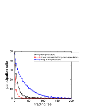
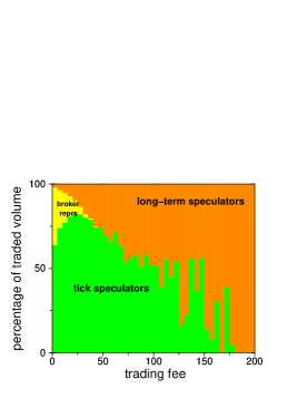
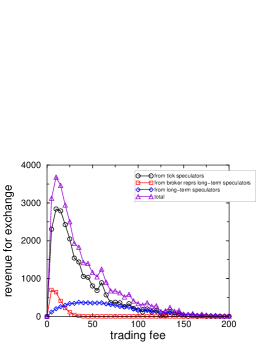
Figure 9: (Colour on-line) Left: Participation ratio for tick-traders, long-term speculators and broker represented long-term speculators versus trading fee. Middle: Relative percentage of total trading volume attributed to each group. Right: revenue for market maker. From [35].

7 Use of information in Minority Games and related models

A further unrealistic simplification is the assumption of uniform available information and equal intellectual capacities of all agents, usually made in simple setups of the MG. More accurate models can here be expected to be more diverse and should account for heterogeneity in these aspects. In particular issues of individually different memory capacities and access to information are here to be considered, the latter leading to models with so-called ‘private information’.

7.1 An agent-based model with private information

A model with private information has been considered in [8] and [26]. Although the model studied there is not directly derived from the MG, it shows similar features. The model is based on the Shapley-Shubik [74] model of markets, and considers limitation to private information explicitly. As in the MG one assumes the existence of a global state of the market $\omega(t)$, which takes one of $P=\alpha N$ values at each time $t$ (with $N$ the number of traders in the market), but that agents have access to this information only through individual information filters $k_{i}^{\omega}$, where $i$ labels the individual agents. On the basis of the external signal $\omega$ agent $i$ receives ‘filtered’ information $k_{i}^{\omega}$ which may hence vary across the population of agents. In the simple setup of [8] and [26] the $\{k_{i}^{\omega}\}$ take only binary values $k_{i}^{\omega}\in\{-1,1\}$. The state $\omega$ is also assumed to determine the (quenched random) return $R^{\omega}$ of an underlying asset traded on the model market. Thus the vector $\mathbf{k}_{i}=(k_{i}^{1},\dots,k_{i}^{P})$ crucially constrains the ability of agent $i$ to resolve different states of the market. If for example $k_{i}^{\omega}=-1$ for all $\omega$ then agent $i$ is completely blind with respect to the actual state of the market, he receives information $-1$ no matter what the actual value of $\omega(t)$ and hence cannot distinguish any two different information patterns. If $k_{i}^{\omega}$ is highly correlated with $R^{\omega}$ (e.g $k_{i}^{\omega}=1$ whenever the return $R^{\omega}$ is positive, and $k_{i}^{\omega}=-1$ for all $\omega$ for which $R^{\omega}$ is negative), then agent $i$ is very well able to distinguish states of the market, and to make accurate predictions on the further price movements.

A detailed statistical mechanics analysis shows that the phase transition of the MG market model is present also in this context, see Fig. 10. There we plot the resulting predictability $H$ as a function of $\alpha$ for different choices of other model parameters (not specified here), note in particular that the model can again be solved exactly (solid lines in the figure). The right panel of Fig. 10 depicts an order parameter $q$ which measures the degree to which agents use their privately obtained information. At the phase transition $q$ is maximal, and the agents’ decisions crucially depend on the information they receive. At large or low values of $\alpha$ much less use of the available information is made, and agents essentially trade independently of the received binary private information.

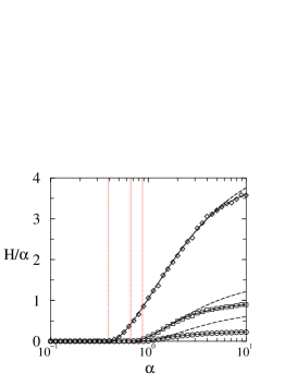
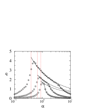
Figure 10: Predictability $H$ and use of information $q$ in a market model with private information. From [26].

7.2 MG with dynamics on heterogeneous time-scales

7.2.1 Heterogeneous time-scales

Agents in real markets can differ in time horizon on which they act and on which they develop their own strategy. This point is often neglected, although there is of course some work stressing this particular aspect of real markets [65]. Very recently LeBaron pointed out that different time scales can be responsible for the appearance of different beliefs on the market and the co-existence of these beliefs helps to generate features across many time scales through symbiotic effects [51]. In MGs there are several ways in which one can implement different time scales among agents, for example through individual learning rates, score memories or strategy correlation [63]. In 2-strategy MGs one can introduce correlation between the strategies of any given agent by the drawing the strategy tables such that

$$P(a^{\mu}_{i,1}=a^{\mu}_{i,-1})=c.$$ (17)

In this setup, with probability $c$, the two strategies of any given player will prescribe the same action as response to the appearance of history $\mu$. Thus, if $c=0$ player $i$’s strategies are fully anti-correlated, $a_{i,1}^{\mu}=-a_{i,-1}^{\mu}$ for all $\mu$. For $c=1/2$ one recovers the MG with uncorrelated strategies. For $c=1$ each players holds two fully correlated (i.e. identical strategies), and is an infinitely ‘slow’ player in the sense that his reaction to a certain information pattern does not change over time. The smaller $c$ the faster are the agents, at least in the simplified picture of this model. In this setup, one is particularly interested in the information ecology of the model, i.e. to understand whether groups of different strategy correlation exploit each other, and can live in symbiosis. If two different groups, say fast and slow, are introduced, with $c_{f}<c_{s}$ where $f,s$ stand for fast and slow, the behaviour is already quite rich and can be studied exactly by means of replica theory. Fig. 11 shows that gains $\gamma_{f},\gamma_{s}$ of fast and slow agents respectively, depend in a highly non-trivial way on the fraction $\phi_{f}$ of fast players and the correlation parameters $c_{f},c_{s}$ .

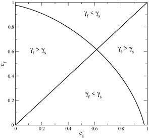
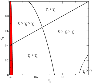
Figure 11: Regions of relative advantage for $\phi_{f}=0.5$ (left graph) and $\phi_{f}=0.01$ (right graph); the region filled corresponds to the symmetric phase, in which the replica calculus is not valid. From [63].

Another way to investigate the role of time scales in MGs is to study the game with just one information pattern (i.e. the limit $P\to 1$) [59, 60]. This limiting case is particularly straightforward to understand analytically. Given $A(t)$ each agent $i$ receives a payoff $-a_{i}(t)A(t)$, and keeps a score $\Delta_{i}(t)$ as follows

$$\Delta_{i}(t+1)=\Delta_{i}(t)-\frac{A(t)}{N},$$ (18)

and his trading action is then determined by the stochastic rule

$$P[a_{i}(t+1)=1]=\frac{1+\Gamma_{i}\Delta_{i}(t)}{2}$$ (19)

with $\Gamma_{i}$ a learning rate. Thus high values of $\Delta_{i}(t)$ favour positive trading action $a_{i}(t+1)=1$ by player $i$. It is then possible to consider $G$ groups of $\phi_{g}N$ agents respectively (with $g=1,\dots,G$ and $\sum_{g=1}^{N}\phi_{g}=1$) with all the agents belonging group $g$ following a learning rule of rate $\Gamma_{g}$. Without going into any detail here, we will just point out that the relative gains of the respective groups can be obtained as

$$\gamma_{g}-\gamma=\frac{\Gamma-\Gamma_{g}}{2(1+\Gamma)}$$ (20)

(within some approximation) where $\gamma_{g}$ is the average gain of players in group $g$, $\gamma$ the gain averaged over all groups, and $\Gamma$ the mean learning rate (over all groups). It is interesting to observe that the smaller $\Gamma_{g}$ the smaller the loss of group $g$. For details and other extensions see [63].

7.2.2 Timing of adaptation

The effects of the timing of adaptation on MGs have been studied for example in [73, 33]. One here distinguishes between so-called ‘on-line’ and ‘batch’ adaptation of the MG agents. In the more usual ‘on-line’ games, agents adapt to the external flow of information instantly, and update their strategy scores at every round of the game, and then choose the trading strategy to use in the next step. In batch games, agents adapt only after a large number of rounds has been played, and the corresponding information regarding the performance of the strategies has been accumulated. An interpolation between both cases is possible. Specifically, one allows the agents to update their scores (and re-adapt their strategy choices) only once every $M$ rounds (with accumulative increments over the past $M$ rounds), i.e.

$$U_{i,s}(t+M)=U_{i,s}(t)-\frac{1}{M}\sum_{\ell=0}^{M-1}a_{i,s}^{\mu(\ell)}A^{\mu(\ell)}[\{U(t)\}].$$ (21)

Their choice of strategy then remains fixed in between two updates (as indicated by the dependence of the total action on the scores at time $t$ in Eq. (21)). The limit $M\to 1$ reproduces the on-line case, the case $M\gg P$ (with $P$ the number of possible values of the information) is referred to as the ‘batch’ game, in which an effective average over all information patterns is performed. While the volatility of standard MGs with uncorrelated strategies is not sensitive to the choice of on-line versus batch dynamics, qualitative differences are found in MGs with fully anti-correlated strategy assignments ($c=0$ in the notation of the previous section), see Fig. 12. Adaptation at randomly chosen time-intervals of mean $M$ finally reduces the volatility in the efficient phase of the market, but not above the phase transition, see Fig. 13.

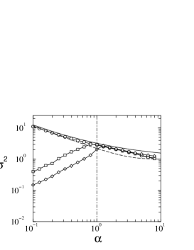
Figure 12: On-line versus batch game for fully anti-correlated strategies. Left: on-line game, started from different initial conditions. Right: batch game. Note the difference in the qualitative behaviour. From [33].

7.3 Cost of information

Ideally one would like to consider models in which agents can acquire information at some cost, i.e in which they pay for the use of expertise. To the knowledge of the authors, no such attempts have yet been made in an analytical statistical mechanics approach. One may also consider models in which agents have both public and private information at their disposal, and have to decide which to use. One may think of globally available information through newspapers and other media, versus the recommendations of a small circle of private advisors and/or friends.

8 Summary and outlook on future work

In summary we have reviewed the recent progress in the description of financial markets through simple agent-based models, accessible by the techniques of theoretical statistical mechanics. The MG in particular can be seen as a minimalist market model, which can be treated analytically in its basic setup and is now considered to be essentially fully understood. While in its original setup of each agent trading one unit at any given time step the MG does not display anomalous fluctuations and stylised facts as seen in real market data, only minor modifications are necessary to make the model more realistic in this sense, without giving up the analytical tractability. MGs with a finite number of agents and with dynamical capitals and/or with an option of the agents to abstain have been shown to display anomalous fluctuations close to their phase transitions, similarly to systems of statistical mechanics exhibiting large scale correlations and self-similarity near their critical points. These observations call for further analysis of such variants of the MG, for example by means of renormalisation group techniques.

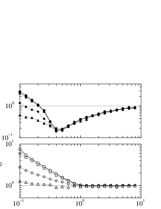
Figure 13: Volatility for model with random updates, probability to update $1/M$. Top panel corresponds to MG with uncorrelated strategy assignments, lower panel to the fully anti-correlated case. From [33].

The MG can also serve as a platform for more diverse market simulations, and an ecology of market participants can be studied upon introducing diversified types of players in the MG. These may include contrarians and trend-followers respectively, as well as agents trading on different time-scales and/or with different trading volumes, and agents of different memory capacities. While it is presumably unlikely that real market trading decisions can be taken on the basis of MG simulations, the model as such and its diverse variants and extensions offer a promising approach to gain a better understanding of the interplay of market parameters and the ecology of populations of traders, based on models at the boundary of analytical solvability. Future research in this direction may thus be of interest both in an academic environment as well as for practitioners.

References

References

- [1] Andersen JV, Sornette D 2003, Eur. Phys. J. B 31 141
- [2] Arthur B 1994, Am. Econ. Assoc. (Papers & Proc.) 84 406
- [3] Arthur WB, Holland J, LeBaron b, Palmer R, Tayler P 1997, in Arthur, Durlauf, Lane, eds, The Economy as an Evolving Complex System II (Addison-Wesley)
- [4] Axelrod R 1997, The Complexity of Cooperation: Agent-Based Models of Competition and Collaboration (Princeton University Press, NJ)
- [5] Bachelier L 1900 Théorie de la Spéculation, Annales Scientifiques de l’Ecole Normale Supérieure
- [6] Bak P 1996 How nature works, Springer-Verlag Telos
- [7] Newman M, Barabasi A-L, Watts DJ 2006 The Structure and Dynamics of Networks, Princeton University Press
- [8] Berg G, Marsili M, Rustichini A, Zecchina R 2001 Quant. Fin 1(2)
- [9] Bianconi G, Galla T, Marsili M 2006, preprint arXiv:cond-mat/0603134
- [10] Bouchaud JF, Giardina I, Mezard M 2001, Quantitative Finance 1 212
- [11] Bouchaud JP, Potters M 2000 Theory of financial Risk, from statistical physics to risk management, Cambridge University press
- [12] Black F, Scholes M 1973, Journal of Political Economy 81 (3) 637
- [13] Cardy JL Scaling and Renormalization in Statistical Physics, Cambridge Lecture Notes in Physics
- [14] Challet D, http://www.unifr.ch/econophysics/minority
- [15] Challet D 2005 arXiv:physics/0502140
- [16] Challet D, Chessa A, Marsili M, Zhang Y-C 2001 Quant. Finance 1 168
- [17] Challet D, Marsili M and Zhang Y-C 2000 Physica A 276 284
- [18] Challet D, Marsili M, Zhang Y-C 2005, Minority Games: Interacting Agents in Financial Markets (Oxford University Press)
- [19] Challet D and Zhang Y-C 1997 Physica A 246 407
- [20] Challet D and Zhang Y-C 1998 Physica A 256 514
- [21] Challet D and Marsili M Phys. Rev. E 68 036132 (2003)
- [22] Challet D, Marsili M, Zhang YC 2001 Physica A 294 514
- [23] Cont R, Bouchaud JF 2000, Macroeconomic Dynamics 4 170
- [24] Coolen ACC 2005, The Mathematical Theory of Minority Games: Statistical Mechanics of Interacting Agents (Oxford University Press)
- [25] Coolen ACC, Heimel J A F and Sherrington D 2001 Phys. Rev. E 65 016126
- [26] De Martino A, Galla T 2005,J. Stat. Mech. P08008
- [27] De Martino A, Giardina I, Marsili M, Tedeschi A 2004 Phys. Rev. E 70 025104(R)
- [28] De Martino A, Giardina I, Mosetti G 2003 J. Phys. A: Math. Gen. 36 8935
- [29] De Martino A, Marsili M 2001 J.Phys. A: Math. Gen. 34 2525
- [30] Ferreira FF, Marsili M 2005, Physica A 345 (3,4) 657
- [31] Frankel JA, Froot KA 1998, in Chambers and Paarlberg, eds, Agriculture, Macroeconomics and the Exchange Rate (Westview Press, Boulder, CO)
- [32] Fischer KA, Hertz JA 1991, Spin Glasses (Cambridge University Press)
- [33] Galla T and Sherrington D 2005 Eur. Phys. J. B 46 153
- [34] Galla T 2006 (forthcoming)
- [35] Galla T and Zhang Y-C 2005, technical report
- [36] Galla T and Zhang Y-C (in preparation 2006)
- [37] Gilbert N, Troitzsch K 2005, Simulation for the Social Scientist, 2nd edition (Open University Press)
- [38] Girdina I, Bouchaud JP 2002 Eur. Phys. J. B 31 421
- [39] Gopikrishnan P, Plerou V, Amaral L, Meyer M, Stanley HE 1999 Phys. Rev. E 60 5305
- [40] Heimel J A F, Coolen A C C 2001, Phys. Rev. E 63 056121
- [41] Helbing D Dynamics of traffic, Springer-Verlag 1997 (in German)
- [42] Helbing D Stochastic methods, non-linear dynamics and quantitative models of social processes, Shaker Verlag 1996 (in German)
- [43] Hommes C 2006,in Leigh Tesfatsion and Kenneth L. Judd, eds,Handbook of Computational Economics Vol. 2: Agent-Based Computational Economics (Elsevier/North Holland)
- [44] Jefferies P, Hart M, Hui P, Johnson N F 2001, Eur. Phys. J. B20 493
- [45] Johnson NF, Hart M, Hui PM, Zheng D 2000, International Journal of Theoretical and applied Finance 3 443
- [46] Johnson NF, Jefferies P, Hui PM 2003, Financial Market Complexity (Oxford University Press)
- [47] Kadanoff LP 2000 Statistical physics, statics, dynamics and renormalisation, World Scientific
- [48] Kozlowski P, Marsili M 2003 J. Phys. A: Math. Gen. 36 11725
- [49] Kirman AP 1991, in M. Taylor, ed., Money and Financial Markets (MacMillan, London)
- [50] LeBaron B, Arthur WB, Palmer R 1999,Journal of Economic Dynamics and Control 23 1487
- [51] Le Baron B 2006, http://people.brandeis.edu/ blebaron/wps/timescales.pdf
- [52] Le Baron B 2006, in Leigh Tesfatsion and Kenneth L. Judd, eds, Handbook of Computational Economics Vol. 2: Agent-Based Computational Economics (Elsevier/North Holland)
- [53] Levy M, Levy H, Solomon S 1994, Economic Letters 45 103
- [54] Liu Y, Goprikishnan P, Cizeau P, Peng CK, Meyer M, Stanley HE 1999, Phys. Rev. E 60 1390
- [55] Levy M, Levy H, Solomon S 2000, Microscopic Simulation of Financial Markets: From Investor Behavior to Market Phenomena (Academic Press)
- [56] Lo AW 1991,Econometrica 59 1279
- [57] Lux T, Marchesi M 1999 Nature 397 498
- [58] Mantegna RN, Stanley HE 2000, An introduction to Econophysics (Cambridge University Press)
- [59] Marsili M 1999, Physica A 299 (1-2) 93
- [60] Marsili M and Challet D 2001 Phys. Rev. E 64 056138
- [61] Marsili M, Challet D and Zecchina R 2000 Physica A 280 522
- [62] Merton RC 1992 Continuous -Time Finance (Macroeconomics and Finance), Blackwell Publishing
- [63] Mosetti G, Challet D, Zhang Y-C 2006, Physica A 365(2) 529
- [64] Newman MEJ 2005 Contemporary Physics 46, 323
- [65] Olsen R et al 1992, Tech. Rep. RBO. 1992-09-07, (Olsen & Associates)
- [66] Pareto V 1896, Cours D’Economie Politique, volume I and II. F. Rouge, Lausanne.
- [67] Parisi G, Mezard M, Virasoro M 1987, Spin Glass Theory and Beyond (World Scientific)
- [68] Raberto M, Cincotti S, Focardi SM, Marchesi M 2001,Physica A 299 319
- [69] Savit R, Manuca R and Riolo R 1999 Phys. Rev. Lett. 82 2203
- [70] Shayeghi N, Coolen ACC 2006, preprint cond-mat/0606448
- [71] Samuelson P 1983 Foundations of Economic Analysis, Enlarged Edition (Harvard University press)
- [72] Schreckenberg M and Wolf D 1998 Traffic and Granular Flow ’97, Springer Verlag, Singapore
- [73] Sherrington D and Galla T 2003 Physica A 324 25
- [74] Shapley L, Shubik M. 1977 Journal of Political Economy 85 937
- [75] Slanina F, Zhang Y-C 1999, Physica A 272 257
- [76] Stanley H 1971, Introduction to Phase Transitions and Critical Phenomena (Oxford University Press)
- [77] A. Tedeschi, A. De Martino, I. Giardina 2005, Physica A 358 529 preprint cond-mat/0503762
- [78] Walras L 1954 Elements of Pure Economics, Allen and Unwin (London)