Evaporative cooling in a radio–frequency trap

Abstract

A theoretical investigation for implementing a scheme of forced evaporative cooling in radio–frequency (rf) adiabatic potentials is presented. Supposing the atoms to be trapped by a rf field at frequency $\omega_{1}$, the cooling procedure is facilitated using a second rf source at frequency $\omega_{2}$. This second rf field produces a controlled coupling between the spin states dressed by $\omega_{1}$. The evaporation is then possible in a pulsed or continuous mode. In the pulsed case, atoms with a given energy are transferred into untrapped dressed states by abruptly switching off the interaction. In the continuous case, it is possible for energetic atoms to adiabatically follow the doubly–dressed states and escape out of the trap. Our results also show that when $\omega_{1}$ and $\omega_{2}$ are separated by at least the Rabi frequency associated with $\omega_{1}$, additional evaporation zones appear which can make this process more efficient.

I Introduction

In recent years, the investigation of quantum gases in low–dimensional trapping geometries has significantly attracted the attention of the physics research community. This growing interest is motivated, partially, by the current possibilities that the extremely rapid progress in integrated atom optics has opened for the manipulation of Bose–Einstein condensed (BEC) atoms. This development allows the study of crucial problems associated with the strong modifications that the fundamental properties of these quantum systems experience due to the reduced dimensionality. For instance, a 1D Bose gas in the Tonks–Girardeau regime mimics a system of non–interacting spinless fermions tonks ; girardeau ; paredes ; in 2D, the superfluidity emerges due to the vortex binding–unbinding Berezinskii–Kosterlitz–Thouless phase transition BKT1 ; BKT2 , recently observed zoran .

For the study of the BEC low–dimensional physics, trapping configurations of different nature and topology have been proposed and used. For example, the 3D to 1D crossover was explored by Görlitz et al. gorlitz in an elongated Ioffe–Pritchard type direct–current (dc) magnetic trap, the phase defects of a BEC were investigated in a quasi–2D trap based on a 1D optical lattice stock and, in atom chip experiments, dc current–carrying wires are usually employed to confine atoms in highly anisotropic traps folman . Although these trapping configurations have demonstrated their relevance for studying quantum gases in low dimensions, adiabatic potentials zobay , resulting from a combination of dc and radio–frequency (rf) magnetic fields, are also becoming a very attractive and promising tool colombe ; schumm ; morizot ; courteille ; lesanovsky ; fernholz .

The rf traps share the versatility and flexibility of the above mentioned trapping schemes and, moreover, they are relatively easy to implement and control. In the first implementation of these traps colombe , ultra–cold atoms were confined in a 2D geometry. A rf adiabatic potential has also been used as a beam splitter, allowing the demonstration of matter–wave interference on an atom chip schumm . Ring–shaped traps, and other more complex trapping geometries using adiabatic potentials have also been considered morizot ; courteille ; lesanovsky ; fernholz .

Given the topology of the rf trapping potential, and because of technical limitations in some cases, the loading of the trap with Bose–Einstein condensed atoms, preserving the quantum degeneracy, can be a challenging task. In this situation, it is of relevance to consider the possibility of evaporative cooling of atoms directly in these low–dimensional rf traps. This is the subject that will be addressed in this paper, taking into account the interaction of the atoms with two radio–frequency fields. When dealing with more than one rf frequency, an analytical solution for the atomic spin dynamics can be found by treating the individual successive interactions of the rf fields with the atoms ramsey or by considering the two fields simultaneously, provided one of the fields is rather weak ficek . We will study how a weak second radio–frequency source can be used to perform an evaporation.

We will see that the forced evaporation of rf–trapped atoms can be accomplished in two ways. Firstly, the spin evolution induced by this second rf source can be quenched by switching off the field, i.e. by using a pulsed rf source. Secondly, we can allow an adiabatic following of doubly–dressed states which requires the second rf source to be continuous rather than pulsed. This last scheme is similar to the standard evaporative cooling method used in static magnetic traps hess ; vitanov ; luiten .

This paper is organized as follows: In section II we will discuss the geometry of the system and the singly–dressed states of the rf trap. In Sec. III, the evolution of the system is determined in three different ways: numerically, using a first order Magnus series approximation, and by using a second rotating wave approximation which leads to a double–dressing of the atoms by two rf fields. Sec. IV is devoted to the application of the results of Sec. III to the study of evaporative cooling in the rf trap. Finally, we give a summary and conclusion in Sec. V.

II Adiabatic potential confinement

The underlying idea of the confinement of ultra–cold atoms using rf adiabatic potentials is presented in detail in Ref. zobay , Ref. colombe being the first report on the experimental investigation of such a trapping scheme. For this reason, instead of discussing deeply how this trapping actually takes place, we will rather make use of the already known results that are relevant in order to consider the problem of evaporative cooling in these traps.

The treatment presented in this paper is valid for any value of the spin $F$. However, for concreteness the numerical results will be given for ⁸⁷Rb in the Zeeman state $m=+2$ of the $5S_{1/2}$, $F=2$ hyperfine ground state level. We will suppose that the atoms are confined in a QUIC magnetic trap esslinger ; lu produced by a dc magnetic field $\textbf{B}_{dc}(\textbf{r})$. The atomic clouds trapped in this configuration are anisotropic (cigar–shaped along $x$) and we will take the offset magnetic field produced by the Ioffe coil esslinger to be oriented along the $x$ direction. In the following, the axes in the lab frame will be labelled by lower case letters $xyz$. The $z$ axis is in the vertical direction and $y$ is the horizontal direction perpendicular to the cigar axis. The axes in the local frame attached to the dc magnetic field will be labelled by capital letters $XYZ$. Moreover, we will assume that the direction of the dc magnetic field defines the local $Z$ quantization axis. The Larmor frequency of the atomic spin precession in this dc field will be denoted $\omega_{0}(\textbf{r})=g_{F}\mu_{B}B_{dc}(\textbf{r})/\hbar$. Here, $g_{F}$ and $\mu_{B}$ are the Landé factor and the Bohr magneton, respectively.

Now, we apply to this confined atomic system two rf fields (produced by antennae), both of them polarized along $X$ and of angular frequencies $\omega_{1}$ and $\omega_{2}$. Having in mind that the second rf field will be rather weaker than the first one, we transform into the frame rotating at $\omega_{1}$ and perform the rotating wave approximation (RWA). The Hamiltonian that describes the spin dynamics can thus be written as (see the derivation in appendix A)

$$H(\textbf{r},t)=H_{A}(\textbf{r})+\Omega_{2}\big{[}F_{X}\cos(\Delta t)+F_{Y}\sin(\Delta t)\big{]}\ ,$$ (1)

where $F_{X}(F_{Y})$ is the atomic angular momentum in the $X(Y)$ direction, $\Delta=\omega_{2}-\omega_{1}$, $H_{A}(\textbf{r})=\Omega(\textbf{r})F_{\theta}$ is the adiabatic Hamiltonian associated with the rf confinement, and $\Omega(\textbf{r})\equiv\sqrt{\delta(\textbf{r})^{2}+\Omega_{1}^{2}}$ defines the energy separation between the adiabatic levels. In the absence of $\Omega_{2}$, the flip angle $\theta$ and the detuning $\delta(\textbf{r})$ are given by $\tan(\theta)\equiv-\Omega_{1}/\delta(\textbf{r})$, with $\theta\in[0,\pi]$, and $\delta(\textbf{r})=\omega_{1}-\omega_{0}(\textbf{r})$, respectively. We have labelled the Rabi frequencies of the rf fields $\Omega_{1}$ and $\Omega_{2}$, and we have considered that the component $F_{Z}$ of the atomic angular momentum is aligned with the local $Z$ component of the dc magnetic field vector. Strictly, these Rabi frequencies are not spatially homogeneous, however they can be treated as such over the spatial extension of the atomic cloud colombe .

Graphically, the spin evolution given by Eq. (1), in the case $\Omega_{2}=0$, is represented in Fig. 1. It can be seen in this figure that the tilted angular momentum $F_{\theta}$ results from a rotation of $F_{Z}$ around $F_{Y}$ and is given by

$$F_{\theta}=\cos(\theta)F_{Z}+\sin(\theta)F_{X}=\mathcal{R}_{Y}(\theta)F_{Z}\mathcal{R}_{Y}^{{\dagger}}(\theta)\ ,$$ (2)

where the rotation matrix $\mathcal{R}_{Y}(\theta)=\exp(-i\theta F_{Y}/\hbar)$ can be expressed in the basis $\{-2,...,+2\}$ of the bare states.

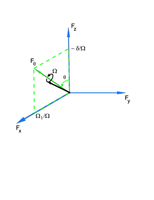
Figure 1: (color online). At a given location r, $\delta$ and $\Omega_{1}$ define the angle $\theta$ by which $F_{Z}$ is rotated. The spin (black arrow) therefore precesses around an axis given by $F_{\theta}$ (green arrow) at a frequency $\Omega$.

In Fig. 2(a), the energies of the bare states are plotted as a function of the position $z$, where the energy variation is due to the dc magnetic field $\textbf{B}_{dc}(\textbf{r})$. This spatial dependence has been calculated for a value $x=x_{min}=6.9$ mm corresponding to the position where the QUIC magnetic field is minimal in our experimental setup colombe . Moreover, we have taken $y=0$ and a Rabi frequency $\Omega_{1}/2\pi=400$ kHz. The arrows shown in that figure, in blue for $\omega_{1}$ and in red for $\omega_{2}$ (each frequency stands to the right of its respective arrows), indicate the locations where the corresponding rf fields resonantly couple the states in the laboratory frame. On the other hand, the spatial $z$ dependence of the adiabatic states internal energies is shown in Fig. 2(b) where the states are labelled, from top to bottom: $|+2_{A}\rangle,\ |+1_{A}\rangle,\ |0_{A}\rangle,\ |-1_{A}\rangle$, and $|-2_{A}\rangle$. We can also see in this last figure the avoided level crossings at the positions where $\omega_{1}$ (taken equal to $2\pi\times$3.19 MHz in this example and from now on) resonantly couples the bare states.

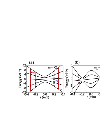
Figure 2: (color online). Spatial $z$ dependence of the energy of the uncoupled (a) and dressed (b) states for $x=x_{min}$ and $y=0$. At the avoided level crossings, the energy splitting between the levels is $\Omega_{1}$. Gravity has been taken into account in both cases and $\omega_{2}>\omega_{1}$.

In order to consider only the confinement ($\Omega_{2}=0$) using the adiabatic potentials shown in Fig. 2(b), let’s suppose that initially we have a $m=+2$ spin polarized ultra–cold atomic sample. In this situation, the trapping potential corresponding to the bare state $|+2\rangle$ can be adiabatically deformed into the one associated with the dressed state $|+2_{A}\rangle$. Such a transformation can be performed by changing the detuning $\delta(\textbf{r})$ from red to blue at constant Rabi frequency $\Omega_{1}$ zobay ; colombe or, by increasing $\Omega_{1}$ at a constant red detuning schumm . Here, by adiabatic deformation we mean that the angular precession frequency $\Omega(\textbf{r})$ of the spin in Fig. 1 must be much larger than the rate at which the angle $\theta$ changes [$|\dot{\theta}|\ll\Omega(\textbf{r})$]. Using the loading schemes just mentioned, it is possible to obtain highly anisotropic rf traps with trapping frequencies, in the strongest confinement direction, ranging from several hundreds of Hz up to a few kHz.

Having described the main properties of the adiabatic confinement, let’s now address the following issues. Assuming intuitively the existence of the resonances represented by the arrows in Fig. 2(b), we would like to know precisely where they are located and how strong they are. Another relevant point to be taken into account concerns the effect of these resonances at the rf trap centre when, numerically, $\omega_{1}$ and $\omega_{2}$ are close to each other. Moreover, it will be interesting to find out the different parameter values for which the second rf field induces transitions between the adiabatic states, in the perturbative limit with $\Omega_{2}\ll\Omega_{1}$, leading to a possible implementation of evaporative cooling in rf traps.

III Dynamics of the system

In this section we will study the dynamics of the system using three different methods. In the first case, the exact numerical solution of the time–dependent Schrödinger equation (TDSE) will be found. Secondly, an approximated analytical treatment will be presented (Magnus approximation) in order to interprete the exact results derived numerically. Finally, we will present an analytic solution based on a second rotating wave approximation which will be the basis of the analysis presented in Sec. IV.

Since the evolution of the atomic external and internal degrees of freedom takes place on very different time scales, here we will decouple the two dynamics and consider only the time evolution of the internal degrees of freedom.

III.1 Numerical solution

The evolution of the state vector $|\Psi(t)\rangle$ with the Hamiltonian (1) was solved numerically, in the interaction picture, using a 4th order Runge–Kutta algorithm. In this case, the state vector can be very efficiently propagated in time and we do not expect to have convergency problems if we choose an appropriate time–step tremblay . The first question we would like to address here is: supposing that an atom is initially in the trapped dressed state $|+2_{A}\rangle$, what is the probability $P_{2A}=|\langle 2_{A}|\Psi(\textbf{r},t)\rangle|^{2}$ of finding it in that same state as time goes by? We will also be interested in how this probability changes for an atom located in different places in the trap. The preliminary answer to these questions is presented in Fig. 3, where the probability we are interested in is plotted for three different values of $\Delta$, the difference between the radio–frequencies $\omega_{1}$ and $\omega_{2}$.

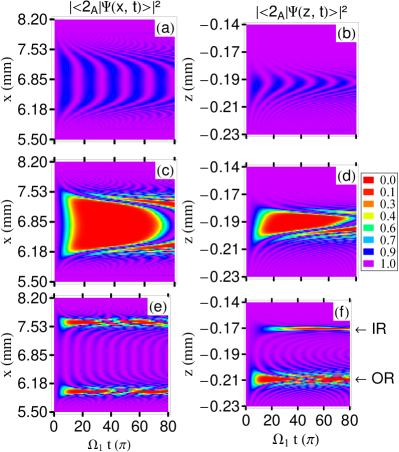
Figure 3: (color online). Probability for an atom to remain in the initial rf trapped state $|+2_{A}\rangle$. The values of $\Delta$ are respectively: 0.875$\Omega_{1}$ in (a) and (b); $\Omega_{1}$ in (c) and (d); and 1.25$\Omega_{1}$ in (e) and (f). The rf trap frequency $\omega_{1}/2\pi$ is set to 3.19 MHz. The $x$-$t$ ($z$-$t$) dependence of $P_{2A}$ is calculated at $z_{min}=-0.19$ mm ($x_{min}=6.9$ mm). In (f) the labels OR and IR indicate the locations of the outer and inner resonances, respectively.

In Fig. 3, and from now on, we use $\Omega_{1}$ as a frequency unit, having in mind to keep it constant in a given experimental situation. The value of $\Omega_{2}$ has been taken equal to 0.05$\Omega_{1}$, small enough in order to be in the perturbative limit, as will be shown later. This value of $\Omega_{2}$ will be used in all the following results unless a different one is explicitly stated. In the left column of Fig. 3, the $x$ and time dependence of $P_{2A}$ are calculated at the points $y=0$ and $z_{min}\approx-0.19$ mm, with this value of $z$ corresponding to the location of the left avoided level crossing in Fig. 2(b). To obtain the right column of figure 3, we use for $x$ the value $x_{min}\approx 6.9$ mm, very close to the location where the QUIC trap has its minimum in the $x$ direction.

In Fig. 3 the three values of $\Delta$ have been chosen to illustrate some key characteristics of the spin dynamics. As the energy separation between the adiabatic levels at the avoided level crossings is exactly $\Omega_{1}$, we observe resonant behaviour at the rf trap bottom for $\omega_{2}=\omega_{1}+\Omega_{1}$, i.e. when $\Delta=\Omega_{1}$ [see Fig. 3(c) and (d)]. Similarly, for $\Delta<\Omega_{1}$ we have a red–detuned interaction everywhere [Fig. 3(a) and (b)]. In this case we observe weak modulations of $P_{2A}$ that are essentially determined by a beating between the $\Delta$ and $\Omega(\textbf{r})$ frequency components. For $\Delta>\Omega_{1}$ [Fig. 3(e) and (f)] we have a blue–detuned interaction around the minima $x_{min}$ and $z_{min}$. Away from the centre a resonance occurs, as expected, at approximately the location in the trap where $\omega_{2}$ resonantly couples the bare states [see Fig. 2(a)]. This is the outer resonance labelled OR in Fig. 3(f). However, there is another feature we would like to stress. Namely, the presence of the inner resonance IR clearly seen in the $z$ dependence of $P_{2A}$ in Fig. 3(f). Note that the avoided level crossing (rf trap centre) is at $z_{min}$. Looking back to Fig. 2 and having in mind that $\omega_{2}>\omega_{1}$, the existence of this second resonance IR in Fig. 3(f) at $z>z_{min}$ may be counter–intuitive and, as we will see, its relative strength is fully determined by the rotation angle $\theta$. Note that because of the loose confinement in the $x$ direction colombe , the dynamics in the $y$-$z$ plane does not change much from one location to another in the $x$ axis. However, this dynamics is very sensitive to changes in $z$ (or $y$) and therefore, the results for the $x$ dependence of the probability $P_{2A}$ in Fig. 3(a), (c), and (e) can be significantly different when another $z$ location is considered.

III.2 Interpreting the numerical results using a first order Magnus series approximation

Searching for the understanding of the physical picture behind the numerical results presented in Fig. 3, let’s consider the first order Magnus series approximation magnus ; milfeld to the solution of the TDSE. This approximation is basically the formal solution of the TDSE neglecting the two–time commutators of the Hamiltonian. This Hamiltonian is given in the interaction picture by

$$H^{{}^{\prime}}(t)=\exp(i\Omega tF_{\theta}/\hbar)H(t)\exp(-i\Omega tF_{\theta}/\hbar)\ .$$ (3)

In Eq. (3), we have dropped the r dependence in $\Omega$ and $F_{\theta}$ for the sake of notational simplification. Making use of Fig. 1 and introducing $F_{\perp\theta}=\mathcal{R}_{Y}(\theta)F_{X}\mathcal{R}_{Y}^{{\dagger}}(\theta)=\cos(\theta)F_{X}-\sin(\theta)F_{Z}$ (see Fig. 6), which is the angular momentum vector perpendicular to $F_{\theta}$ and $F_{Y}$, we find

$$H^{{}^{\prime}}(t)=\Omega_{2}\Big{\{}\sin(\theta)\cos(\Delta t)F_{\theta}+\big{[}\sin(\Delta t)\sin(\Omega t)+\cos(\theta)\cos(\Delta t)\cos(\Omega t)\big{]}F_{\perp\theta}+$$

$$\big{[}\sin(\Delta t)\cos(\Omega t)-\cos(\theta)\cos(\Delta t)\sin(\Omega t)\big{]}F_{Y}\Big{\}}\ .$$ (4)

In this case, the time evolution of a given initial dressed spin state $|\Psi(0)\rangle$ is represented by the rotation

$$|\Psi(t)\rangle=\exp(-i\ \mathbf{\Xi}(t)\cdot\textbf{F}/\hbar)|\Psi(0)\rangle\ ,$$ (5)

where the scalar product $\mathbf{\Xi}(t)\cdot\textbf{F}$ stands for $\Xi_{\theta}(t)F_{\theta}+\Xi_{\perp\theta}(t)F_{\perp\theta}+\Xi_{Y}(t)F_{Y}$, where $\Xi_{\theta}(t)$, $\Xi_{\perp\theta}(t)$ and $\Xi_{Y}(t)$ are a measure of the projections of the spin $|\Psi(t)\rangle$ precession axis onto the axes $F_{\theta}$, $F_{\perp\theta}$, and $F_{Y}$, respectively (for simplicity we will just call them projections). Taking into account the equation (4), the definition of the exponential argument in Eq. (5) is

$$\mathbf{\Xi}(t)\cdot\textbf{F}=\int_{0}^{t}dt^{{}^{\prime}}H^{{}^{\prime}}(t^{{}^{\prime}})\ ,$$ (6)

leading to the following expressions for the projections

$$\Xi_{\theta}(t)=\frac{\Omega_{2}}{\Delta}\sin(\theta)\sin(\Delta t)\ ,$$ (7)

$$\Xi_{\perp\theta}(t)=\Omega_{2}\Big{\{}\cos^{2}(\theta/2)\frac{\sin[(\Delta-\Omega)t]}{\Delta-\Omega}-\sin^{2}(\theta/2)\frac{\sin[(\Delta+\Omega)t]}{\Delta+\Omega}\Big{\}}\ ,$$ (8)

$$\Xi_{Y}(t)=2\Omega_{2}\Big{\{}\cos^{2}(\theta/2)\frac{\sin^{2}[(\Delta-\Omega)t/2]}{\Delta-\Omega}+\sin^{2}(\theta/2)\frac{\sin^{2}[(\Delta+\Omega)t/2]}{\Delta+\Omega}\Big{\}}\ .$$ (9)

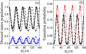
Figure 4: (color online). Occupation probability of the dressed states $|2_{A}\rangle$ (black upper traces) and $|0_{A}\rangle$ (blue lower traces) (a). In (b) the probability for an atom to be in the untrapped dressed states is shown. The circles show exact numerical results (Sec. III.1), the dashed lines from the Magnus approximation (Sec. III.2), and the solid lines from the second RWA (Sec. III.3). The calculation has been done at the rf trap bottom ($x_{min},0,z_{min}$) for $\Delta=1.05\Omega_{1}$ and $\Omega_{2}=0.05\Omega_{1}$.

By inspecting Eqs. (7)–(9), we can see the time–dependent terms resulting from a beating between frequency components at $\Delta$ and $\Omega(\textbf{r})$. These beats are seen as the modulation (interference–like patterns) of $P_{2A}$ observed in Fig. 3. In particular, we see in these equations that there will be some interesting behaviour when $\Delta=\pm\Omega$. In either case the condition is realized by two values of $\theta$: $\theta_{0}$ and $\pi-\theta_{0}$ with $\theta_{0}=\arcsin(\Omega_{1}/\Delta)$. If $\Delta\neq\pm\Omega$, the coefficients $\Xi_{i}(t)$ are oscillatory with finite amplitudes. However, when $\Delta=\Omega$ at $\theta=\theta_{0}$, for instance, $\Xi_{\perp\theta}(t)$ shows a linear tendency in time of the form $\Omega_{2}\cos^{2}(\theta_{0}/2)t$ while the other two components are negligible. This suggests that the spin will essentially rotate at a frequency $\Omega_{2}\cos^{2}(\theta_{0}/2)$ around the axis $F_{\perp\theta}$. Starting from an eigenstate of $F_{\theta}$, as in Sec. III.1, the spin will be completely flipped after a half period. This rotation corresponds to the outer resonance OR in Fig. 3(f). At the location $\theta=\pi-\theta_{0}$, the same resonant behaviour occurs with a rotation frequency $\Omega_{2}\sin^{2}(\theta_{0}/2)$. This corresponds to the inner resonance IR in Fig. 3(f). In the case when $\omega_{2}$ is smaller than $\omega_{1}$, we have the resonant condition $\Delta=-\Omega$ and we have the same behaviour except that the character of the inner and outer resonances is now reversed.

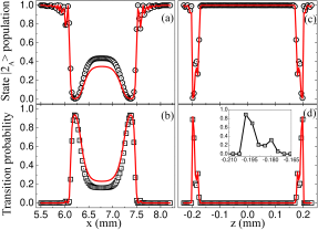
Figure 5: (color online). Population of the dressed state $|2_{A}\rangle$ versus position in the $x$ (a) and $z$ (c) directions at $\Omega_{1}t=20\pi$. The probability for an atom to be in the untrapped dressed states is shown in (b) for the $x$ and in (d) for the $z$ spatial dependence (solid line – Magnus solution, circles and squares – numerical solution). As before, $\Delta=1.05\Omega_{1}$ and $\Omega_{2}=0.05\Omega_{1}$. The inset shows a zoom of the resonances around the avoided level crossing at $z_{min}\approx-0.19$ mm. The solid line in the inset is just to guide the eyes.

Away from the resonant conditions just described the analysis of Eqs. (7)–(9) is more complicated and consequently we evaluate these equations numerically. Some results for the time evolution of the populations of the adiabatic states $|0_{A}\rangle$ and $|2_{A}\rangle$ are given in Fig. 4. We show both Magnus approximation (dashed lines) and the exact numerical solution (circles) for comparison. As can be seen, if we constrain the dressed spin dynamics to half of the first period, we obtain a very good agreement between the first order Magnus series and the exact numerical results. After this time we see dephasing between the two evolutions and, even more dramatic, an important disagreement in the amplitude of the observed oscillations. These two behaviours are somehow expected because at time instants very far from $t=0$ the contribution of the next order terms in the Magnus series becomes more relevant milfeld . In Sec. III.3 we can find a better approximation (using a second RWA) to the numerical solution which is shown in Fig. 4 with solid lines.

Another test for the validity range of the first order Magnus series approximation is presented in Fig. 5, where the population of the dressed state $|2_{A}\rangle$ and the probability of leaving the rf trap are shown. In this figure the results of the numerical treatment and those from the Magnus series are represented by the points and the solid lines, respectively. To obtain the results in Fig. 5, the initial adiabatic spin state has evolved during a time interval approximately equal to one half of the first oscillation period observed in Fig. 4, in short, up to $\Omega_{1}t=20\pi$ that is $t=\pi/\Omega_{2}$. Besides the good agreement that both methods show in the regions of less interest for us, we can notice the four resonances in the $z$ dependence. The inner peaks are rather smaller than the outer ones, indicating that we have a position–dependent resonant coupling.

III.3 Effective Hamiltonian from a second rotating wave approximation

The first order Magnus approximation predicts well the location of the resonances and their spin rotation frequency. However, it fails to describe correctly the dynamics away from the resonance points $\Delta=\pm\Omega$. To tackle this problem, we used a different approach and derived more generally applicable analytical expressions. The approach is based on a second rotating wave approximation, performed on Eq. (1) and expressed through the rotation $\overline{H}(t)=\mathcal{R}_{\Delta}H(t)\mathcal{R}_{\Delta}^{{\dagger}}$ where $\mathcal{R}_{\Delta}=\exp(i\Delta tF_{\theta}/\hbar)$. This transformation leads to the time–dependent Hamiltonian $\overline{H}(t)$ given by

$$\overline{H}(t)=-\big{[}\Delta-\Omega-\Omega_{2}\sin(\theta)\cos(\Delta t)\big{]}F_{\theta}+\Omega_{2}\big{[}\cos(\theta)\cos^{2}(\Delta t)+\sin^{2}(\Delta t)\big{]}F_{\perp\theta}+$$

$$\Omega_{2}\big{[}1-\cos(\theta)\big{]}\sin(\Delta t)\cos(\Delta t)F_{Y}\ ,$$ (10)

where all the parameters appearing in it have already been introduced. We note that this equation is valid for any value of $\Delta$, including those close to $\Omega_{1}$, i.e., when $\omega_{1}$ and $\omega_{2}$ are not so different from each other. Now we apply a second rotating wave approximation, which is valid provided that the “detuning” $\Delta-\Omega$ and the maximum coupling $\Omega_{2}$ are much less than the “carrier frequency” $\Delta$. We finally obtain from Eq. (10) the effective Hamiltonian

$$\overline{H}_{\Delta}=-(\Delta-\Omega)F_{\theta}+\frac{\Omega_{2}}{2}\big{[}1+\cos(\theta)\big{]}F_{\perp\theta}\ .$$ (11)

This last equation provides a new compact and powerful description of the spin dynamics in the dressed trap in the presence of a second rf field. As an example we have shown in Fig. 4 the spin evolution (solid lines) predicted with the effective Hamiltonian which is in excellent agreement with the exact numerical calculations.

The form of the effective Hamiltonian (11) is completely equivalent to that of $H_{A}$ in Eq. (25). If we look, for instance, at the vectorial representation of the spin in the case of a single rf field (Fig. 1), then in the presence of the second rf field one gets the picture shown in Fig. 6, where now $F_{\theta\Delta}=\cos(\theta_{\Delta})F_{\theta}+\sin(\theta_{\Delta})F_{\perp\theta}$ plays a similar role as $F_{\theta}$ did before. The angle $\theta_{\Delta}$ is then

$$\tan(\theta_{\Delta})\equiv-\frac{\Omega_{2}\big{[}1+\cos(\theta)\big{]}}{2(\Delta-\Omega)}\ ,\ \mbox{with}\ \theta_{\Delta}\in[0,\pi]\ .$$ (12)

We can view the resulting precession as a second dressing of the dressed spin states ficek . One can obtain the doubly–dressed states by diagonalizing the Hamiltonian (11). The corresponding eigenenergies of these states are given by multiples of $\hbar\Omega_{\Delta}$ where clearly

$$\Omega_{\Delta}=\sqrt{(\Delta-\Omega)^{2}+\frac{\Omega_{2}^{2}}{4}\big{[}1+\cos(\theta)\big{]}^{2}}\ .$$ (13)

The spin oscillation frequency observed in Fig. 4 is precisely $\Omega_{\Delta}$. On resonance, the period of these Rabi oscillations induced by the coupling in (11) is then $T=4\pi/\Omega_{2}\big{[}1+\cos(\theta)\big{]}$ in agreement with the prediction of the Magnus approximation.

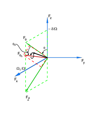
Figure 6: (color online). In the presence of the second rf field and applying a second RWA, the spin (black arrow) precesses around an axis obtained when: Firstly, $\omega_{1}$ tilts $F_{Z}$ by $\theta$ getting $F_{\theta}$. Secondly, $\omega_{2}$ tilts $F_{\theta}$ by $\theta_{\Delta}$ getting $F_{\theta\Delta}$.

Looking at Fig. 6 we realize that $\theta_{\Delta}=\pi/2$ corresponds to resonant coupling with a maximum transition probability to a state orthogonal to the eigenstates of $F_{\theta}$. This happens when $\Omega=\Delta$ [see Eq. (12)]. As in the Magnus case, this condition is realized by the two values $\theta_{0}=\arcsin(\Omega_{1}/\Delta)$ and $\pi-\theta_{0}$ with $\theta_{0}\in[0,\pi/2]$. Recalling that when $\theta=\pi/2$ we are exactly at the avoided level crossings in Fig. 2(b), $\theta_{0}$ indicates the location of the outer resonances OR while $\pi-\theta_{0}$ takes care of the inner ones IR.

IV Evaporation

IV.1 General remarks

In the following two subsections we will consider two schemes for implementing the evaporative cooling. Firstly, we will look at a pulsed scheme in which a fraction of the atoms are spin flipped out of the trapped state by a sudden switch off of the second rf field. Then, secondly, we will examine a continuous scheme in which hot atoms are removed from the rf trap by adiabatically following a doubly–dressed state. In both these schemes the hot atoms that are going to be removed have to reach the resonances at $\theta_{0}$ or $\pi-\theta_{0}$. If we can neglect the gravitational potential, the energy of these atoms should be larger than about $F\hbar(\Delta-\Omega_{1})$ with respect to the bottom of the dressed rf trap. This approximation, valid for relatively small $\Omega_{2}$, can be refined using Eq. (13) and taking gravity into account. As an example, for our typical experimental setup colombe and $\Omega_{2}=0.05\Omega_{1}$, this energy is equivalent to temperatures of 0.21, 6.1 and 11 $\mu$K for $\Delta$ equal to 1.05$\Omega_{1}$, 1.25$\Omega_{1}$ and 1.4$\Omega_{1}$, respectively.

These limiting energies imply, of course, that the atom cloud will have a finite size determined by the location of the inner and outer resonances. In Fig. 7 we investigate the distance $\Delta z_{Res}$ between the neighbouring inner and outer resonances as a function of $\Delta$. As expected, the distance between the resonances goes to zero when $\Delta$ is reduced. In fact, since $\Omega_{2}\ll\Delta$, and if we assume a constant magnetic field gradient $b^{\prime}$, we can derive the approximate form of $\Delta z_{Res}$ from $\Delta=\Omega$ as

$$\Delta z_{Res}=2\frac{\sqrt{\Delta^{2}-\Omega_{1}^{2}}}{\alpha}\ ,$$ (14)

where $\alpha=g_{F}\mu_{B}b^{\prime}/\hbar$.

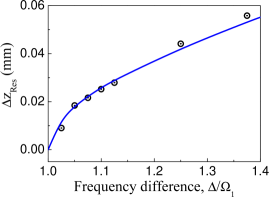
Figure 7: (color online). Distance between neighbouring inner and outer resonances around an avoided level crossing. The circles are from the numerical calculation and the solid line is obtained using Eq. (14) with $b^{\prime}=203$ Gauss/cm. The points were obtained at $t=\pi/\Omega_{2}$ by measuring the distance between the resonances as seen in the inset of Fig. 5(d).

The last point we would like to consider here concerns the inner resonance observed in the $z$ direction. One positive aspect about this resonance is that when $\Delta$ is such that both the inner and outer resonances are close to the bottom of the dressed rf trap, the atomic cloud trapped in the adiabatic state $|2_{A}\rangle$ can be evaporated from both sides. However, the negative point is that some atoms are transferred by the inner resonance into the state $|-2_{A}\rangle$ and trapped around $z=0$. If these atoms come back to the region of the avoided level crossing, then they will be energetic enough that heating of the coldest atoms will take place via inter–atomic collisions. Note that for the rf dressed trap geometry discussed here gravity favours the evaporation through the outer resonance because a lower atomic energy is required than for the inner resonance.

IV.2 Pulsed evaporative cooling

We first look at the pulsed evaporation scheme, which has as its main idea the extraction of hot atoms, in a controlled way, from the rf trap at the resonance locations. We can do this because at these locations we have large transition probabilities between the rf dressed states as seen in Figs. 3(e), (f). These transitions have been already analyzed, firstly, by using the Magnus approximation (Sec. III.2) and, secondly, by using the second RWA (Sec. III.3). They have also been interpreted with the vector picture in Fig. 6 as rotations about $F_{\theta\Delta}$. Hence we can see that if at a given time instant $t$ the precession axis of $|\Psi(t)\rangle$ has zero projection onto $F_{\theta}$, then this state vector will be orthogonal to the initial dressed rf state and consequently, a transition has taken place. Clearly, the second rf field can transfer hot atoms out of the initial trapped dressed state. The pulse has to be repeated several times during the trap oscillation period to ensure an efficient evaporation of all the atoms with sufficient energy to reach the resonances. The pulsed evaporative cooling scheme requires that we can discriminate between hot and cold atoms by affecting as little as possible the atoms in the region of the rf trap centre. This implies a careful choice of the pulse duration and amplitude as will be discussed below.

We already noted that in some situations it may not be desirable to evaporate via the inner resonance (Sec. IV.1). One way we can avoid this resonance in the pulsed scheme is to carefully chose the time duration of the pulse. For example, we can see in Fig. 3(f) that the depletion at the inner resonance (IR) takes place later compared to the outer resonance (OR). This happens because, independently of the orientation of the dc magnetic field, the coupling with the Rabi frequency $\Omega_{2}$ in (11) is spatially inhomogeneous since $\theta$ depends on r. To investigate this inhomogeneity for different values of $\Delta$, we have chosen in Fig. 8 a particular value $t=\pi/\Omega_{2}$ and explore the ratio of the probability of being in the untrapped states at the two resonances. This is shown in the figure as a function of the frequency difference $\Delta$. The second RWA can predict this relative effectiveness of the inner and outer resonances. From Eq. (11) this ratio can be determined analytically for $\Delta=\Omega$ and it is plotted in Fig. 8 with a solid line. The calculation of the numerical results in Fig. 8 is done as follows. For a given value of $\Delta$ a figure similar to Fig. 5(d) is plotted. Then, the ratio of the inner peak height to the outer peak height is found. This is the coupling strength ratio we are interested in. Since there is an excellent agreement between the exact solution and the solid line in Fig. 8, we can state that indeed the second RWA works well in the parameter range we have explored. Notice that for $\Delta\gg\Omega_{1}$ we recover the expected result that only the resonant coupling at the frequency $\omega_{2}$ will occur between the bare states. For intermediate values of $\Delta$, we can clearly see that the particular choice $t=\pi/\Omega_{2}$ for the pulse duration allows a good discrimination between the resonances IR and OR. In the final evaporation stage, where $\Delta\gtrsim\Omega_{1}$, if we wish to limit the IR excitation it is necessary to adapt the pulse duration.

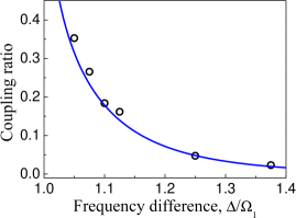
Figure 8: (color online). Ratio between the coupling strengths at the locations of the inner and outer resonances. The exact numerical solution is represented by the points whereas the solid line is derived from the second RWA with $\Delta=\Omega$. For $\Delta$ large compared to $\Omega_{1}$, the coupling at the inner resonances goes to zero.

As mentioned above we should avoid introducing transitions at the dressed rf trap centre. Because of such transitions we can see in Figs. 3(a), (b), (e) and (f) that, even when the detuning for coupling adiabatic states is red or blue ($\Delta<\Omega_{1}$ or $\Delta>\Omega_{1}$), the population of the initial trapped dressed state $|2_{A}\rangle$ is in fact modulated at the centre of the rf trap (avoided level crossing). Such a modulation can produce unwanted heating or losses and, to study this process, we introduce the modulation depth. This quantity is defined as the contrast of the oscillations presented in Fig. 4(a) as the black points (numerical result). In Fig. 9 we plot the modulation depth as a function of the Rabi frequency of the evaporation rf field, and for two different values of $\Delta$. As expected, the modulation depth increases with $\Omega_{2}$ since larger rf power is available for coupling the adiabatic states. Also not very surprising, this modulation is more pronounced when $\Delta$ is such that $\omega_{2}$ couples adiabatic states close to the position of the avoided level crossing.

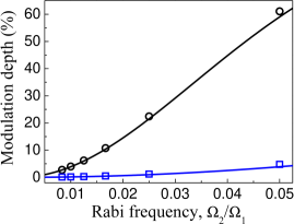
Figure 9: (color online). Modulation of the dressed state $|2_{A}\rangle$ population at the trap centre for $\Delta=1.05\Omega_{1}$ (black open circles) and 1.25$\Omega_{1}$ (blue open squares). The solid lines are calculated analytically from the second RWA treatment.

Taking into account the result presented in Fig. 9, we devised a strategy which affects as little as possible the coldest atoms, while doing the evaporation. The idea is to ramp $\Omega_{2}$ and $\Delta$ simultaneously to preserve a fixed modulation depth at the rf trap centre strat . In Fig. 10 such a ramp is presented, where we have allowed for a 3% modulation level of the coldest atoms population. Note that the reduction of $\Omega_{2}$ has to be taken into account for the optimization of the pulse duration.

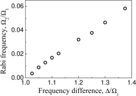
Figure 10: Optimized Rabi frequency as a function of the frequency difference $\Delta$. In this optimization, the population modulation at the rf trap centre is limited to 3%.

In fact, since $\Omega_{2}$ and $\Delta$ can be controlled independently, we can make individual ramps for each one of these parameters and manipulate independently the position and strength of the evaporation resonances. Taking into account that there is a finite modulation of the atomic population at the rf trap centre, even for $\Delta$ very different from $\Omega_{1}$, we propose to use a limited number of rf pulses to cool down the sample. For example, a pulsed evaporative cooling scheme has been developed demonstrating the achievement of the collisional regime in a beam of neutral atoms lahaye . However, this pulsed scheme uses pulses longer than the trap oscillation period unlike the scheme proposed here.

IV.3 Continuous evaporative cooling

Our second scheme for the evaporative cooling of atoms in the dressed rf trap uses the second rf field in a continuous rather than pulsed mode. This situation is closer to the normal case of the evaporation of atoms in a dc magnetic trap by a single rf field. Here, we simply use the second rf field as a tool to control the dressed rf trap depth. This trap depth corresponds to the energy required to reach the resonances (with respect to the dressed rf trap bottom) as considered in Sec. IV.1.

In the usual case of continuous rf evaporation it is useful to look at the system using dressed states. In our situation, the equivalent relevant basis is given by doubly–dressed states. As remarked earlier, these are found by diagonalizing $\overline{H}_{\Delta}$, Eq. (11), or we can write

$$\overline{H}_{\Delta}=\Omega_{\Delta}F_{\theta\Delta}\ ,$$ (15)

with the frequency $\Omega_{\Delta}$ as given in Eq. (13). This frequency determines the doubly–dressed potential $\hbar\Omega_{\Delta}(\mathbf{r})$ which we would like the atoms to follow for the evaporation to proceed. If we include gravity the resulting potential $V_{\Delta}(\textbf{r})$ is given by

$$V_{\Delta}(\textbf{r})=-F\hbar\Omega_{\Delta}(\mathbf{r})+Mgz\ .$$ (16)

An example of this potential is given in Fig. 11 which shows the minimum at $z=z_{min}$ (i.e. at $\theta=\pi/2$ or $\delta=0$), where the cold atoms will eventually collect, as well as the resonance regions IR and OR which form the “lips” of the doubly–dressed trap over which the hotter atoms must pass. (During the usual evaporation process the “lips” are subsequently lowered by ramping the rf frequency and the same procedure can be carried out here with the second rf field.)

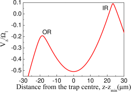
Figure 11: (color online). Doubly–dressed potential $V_{\Delta}$ shown as a function of distance $z-z_{min}$ from the dressed rf trap centre at $z_{min}$ for $\Omega_{2}=0.05\Omega_{1}$ and $\Delta=1.25\Omega_{1}$ as in Figs. 3(e) and (f). The potential is only shown in the region of the singly dressed rf resonance where $\delta=0$, with the associated inner and outer doubly–dressed resonances indicated with IR and OR as in Fig. 3(f). Only the relevant, i.e. lowest, state is shown for $F=2$ and gravity was taken into account in this figure. The vertical unit corresponds to about 20 $\mu$K for the value of $\Omega_{1}$ given in Sec. II.

For this picture to be valid, we must have an adiabatic following of the vector $F_{\theta\Delta}$ as the atoms move about the trap. A general condition for this can be expressed as

$$\Big{|}\frac{d\theta_{\Delta}}{dt}\Big{|}\ll\Omega_{\Delta}\ ,$$ (17)

where $\theta_{\Delta}$ is given in Eq. (12) and the right–hand member of the inequality (17) is seen to be just the energy separation between the doubly–dressed levels. In practice this condition is rather easily satisfied for a singly dressed rf trap (see, for example, Ref. colombe ), which is relevant for the bottom of the doubly–dressed trap as illustrated in Fig. 11. However, in order to also satisfy the adiabatic following condition (17) at the resonances, we will find a new constraint that $\Omega_{2}$ should not be too small. The analysis of adiabaticity is conveniently carried out in terms of a Landau-Zener parameter $\Lambda$ such that Eq. (17) implies that $\Lambda\gg 1$. To proceed, we use the definition (12) of $\theta_{\Delta}$ in order to compute its time derivative assuming that only $\theta$ is time–dependent. Calculating the time derivative and evaluating (17) at the outer resonance location $\theta_{0}$, we find that in terms of the Landau–Zener parameter $\Lambda=\Omega_{\Delta}/|\dot{\theta}_{\Delta}|$ the adiabatic following condition reads

$$\Lambda=\frac{\Omega_{2}^{2}\big{[}1+\cos(\theta_{0})\big{]}^{2}}{4|\dot{\delta}_{0}|\cos(\theta_{0})}\gg 1\ ,$$ (18)

where $\dot{\delta}_{0}$ is the time derivative of the detuning $\delta(\textbf{r})$ evaluated at $\theta_{0}$, and is proportional to an atom velocity. From the expression for $\Lambda$ we can see that as soon as $\Omega_{2}$ is reduced, only the slow atoms will have their spin adiabatically following the axis $F_{\theta\Delta}$, and in fact, for motion linearized over the resonance, the multi-state Landau-Zener analysis vitanov shows that the probability for an atom to be lost from the adiabatic state in a single pass is $1-[1-\exp(-\pi\Lambda)]^{2F}$. For the parameters of Fig. 11, the energy of the atoms $E$ (measured from the trap bottom in temperature units) would have to have a value of $E/k_{B}=20$ $\mu$K for the probability of a non–adiabatic crossing to reach about $10^{-5}$ for the outer resonance OR.

It is clear that if we switch from the outer resonance OR (at $\theta=\theta_{0}$) to the inner resonance IR (at $\theta=\pi-\theta_{0}$) the adiabaticity condition (18) will be different. This is connected to both the spatially dependent coupling $\Omega_{2}\big{[}1+\cos(\theta)\big{]}/2$, and the effect of gravity, which as seen in Fig. 11 make the IR “lip” higher. The weaker coupling at the inner resonance also means that the dynamics is less adiabatic at this point. In fact for fairly “hot” atoms one can contrive that the resonance OR is rather adiabatic whilst the resonance IR is rather diabatic. Together with the effect of gravity, this would mean that atoms can be evaporated out of the OR resonance whilst adiabatic coupling through the IR resonance is prevented. As explained in Sec. IV.1 this can be useful to partially prevent the return of evaporated atoms to the resonance regions with subsequent collisions and heating. However, we note that if we want to reduce the final temperature by steadily reducing $\Delta$, the couplings at the two resonances become more equal (as in the pulsed scheme) and less discrimination between the two evaporation zones is possible.

V Conclusions

We have seen that we can employ a doubly–dressed basis ficek for the analysis of a dressed rf trap with two rf fields provided the second rf field is sufficiently weak. Using this arrangement of fields we can create a scheme for the evaporative cooling of atoms in a singly dressed rf trap in a continuous mode. In contrast with the traditional continuous forced evaporation scheme the idea of evaporative cooling based on the application of rf pulses with properly chosen durations and frequencies is also developed for a dressed rf trap. The duration of such pulses is essentially determined by the power of the rf field used for the evaporation, although the optimal pulse length changes from one location to another in the adiabatic trapping potential. When the trapping and evaporative cooling radio–frequencies are comparable, we found the evaporation to happen also via additional resonances. Even if these resonances can enhance the evaporation process in both the pulsed and continuous schemes, we have to be careful that atoms evaporated through these resonances do not come back and heat the cold atomic cloud. In this respect, the advantage of the pulsed scheme is to provide an additional control of the transition probability at the inner resonance via the pulse duration. However, the effect of gravity is to favour the evaporation via the outer resonance OR which is then located at a position of lower energy. Although the importance of this effect may depend on the particular trapping geometry (pancake, ring traps), the evaporation schemes proposed in this paper are quite general and should allow an efficient cooling of atoms directly in the various rf traps which have been proposed or realized colombe ; schumm ; morizot ; courteille ; lesanovsky ; fernholz .

The main application of the work in this paper is to the evaporative cooling of atoms in a dressed trap. However, there are also applications concerning noise and stability of dressed rf traps where the carrier frequency $\omega_{1}$ is not perfectly monochromatic. This can be due, for instance, to contamination by stray fields. Then it is clear that if the frequency components next to the carrier are in the range of, let’s say, $\Delta=1.01\Omega_{1}$ – $1.05\Omega_{1}$, they will empty the rf trap if they have enough power to do so or, in the best case, they will raise the temperature of the atoms. This means that if we look at the second rf source as a noise term (a sideband in the frequency spectrum), the results presented here can be used to estimate the damage it causes.

Appendix A Derivation of $H(\textbf{r},t)$

We will start the derivation of Eq. (1) by considering that the total magnetic field experienced by the atoms consists of three contributions or terms. One coming from the inhomogeneous dc magnetic field $\textbf{B}_{dc}(\textbf{r})$ of the QUIC trap, a second term oscillating at the frequency $\omega_{1}$, $\textbf{B}_{1}(\textbf{r},t)=B_{01}\textbf{e}_{1}\cos(\omega_{1}t)$, associated with the adiabatic trapping potential, and a third term of frequency $\omega_{2}$, $\textbf{B}_{2}(\textbf{r},t)=B_{02}\textbf{e}_{2}\cos(\omega_{2}t)$, responsible for the evaporative cooling in the rf trap. Here, $B_{01}$ and $B_{02}$ are the amplitudes of the fields whereas $\textbf{e}_{1}$ and $\textbf{e}_{2}$ are unit polarization vectors. Using these definitions and denoting by F the atomic angular momentum operator, the total Hamiltonian of our physical system $H_{T}(\textbf{r},t)$ can be approximated by

$$H_{T}(\textbf{r},t)=g_{F}\mu_{B}\textbf{F}\cdot\big{[}\textbf{B}_{dc}(\textbf{r})+\textbf{B}_{1}(\textbf{r},t)+\textbf{B}_{2}(\textbf{r},t)\big{]}/\hbar\ ,$$ (19)

where $g_{F}$ and $\mu_{B}$ are the Landé factor and the Bohr magneton, respectively. If we assume that at every point r the direction of the dc magnetic field defines the local $Z$ quantization axis then, for $X$ polarized rf fields, the Eq. (19) takes the form

$$H_{T}(\textbf{r},t)=\omega_{0}(\textbf{r})F_{Z}+V_{1}(\textbf{r},t)+V_{2}(\textbf{r},t)\ .$$ (20)

In (20) $\omega_{0}(\textbf{r})=g_{F}\mu_{B}B_{dc}(\textbf{r})/\hbar$ is the Larmor precession frequency. The interaction Hamiltonian $V_{j}(\textbf{r},t)$ is defined by the expression

$$V_{j}(\textbf{r},t)=\Omega_{j}(\textbf{r})F_{X}\big{(}e^{i\omega_{j}t}+e^{-i\omega_{j}t}\big{)}\ \ \ ,\ \ \ j=1,2$$ (21)

being $\Omega_{j}(\textbf{r})\equiv g_{F}\mu_{B}B_{0j}/(2\hbar)$ the Rabi frequency.

Given $H_{T}(\textbf{r},t)$, the dynamics of an atomic spin state $|\phi(\textbf{r},t)\rangle$ is governed by the Schrödinger equation

$$i\hbar\frac{d|\phi(\textbf{r},t)\rangle}{dt}=H_{T}(\textbf{r},t)|\phi(\textbf{r},t)\rangle\ ,$$ (22)

which in the frame rotating at the frequency $\omega_{1}$ becomes

$$i\hbar\frac{d|\psi(\textbf{r},t)\rangle}{dt}=\big{[}-\delta(\textbf{r})F_{Z}+$$

$$\mathcal{R}^{{\dagger}}_{1}V_{1}(t)\mathcal{R}_{1}+\mathcal{R}^{{\dagger}}_{1}V_{2}(t)\mathcal{R}_{1}\big{]}|\psi(\textbf{r},t)\rangle\ .$$ (23)

In Eq. (23) we have introduced the detuning $\delta(\textbf{r})=\omega_{1}-\omega_{0}(\textbf{r})$, the rotating frame operator $\mathcal{R}_{1}=\exp(-i\omega_{1}tF_{Z}/\hbar)$, and the rotated state $|\psi(\textbf{r},t)\rangle=\mathcal{R}^{{\dagger}}_{1}|\phi(\textbf{r},t)\rangle$. If we consider the bare state basis $\{|-2\rangle,|-1\rangle,|0\rangle,|+2\rangle,|+1\rangle\}$ of a spin–2 system, the matrix form of the rotated interaction Hamiltonians $\mathcal{R}^{{\dagger}}_{1}V_{1}(t)\mathcal{R}_{1}$ and $\mathcal{R}^{{\dagger}}_{1}V_{2}(t)\mathcal{R}_{1}$ are respectively given by

$$\Omega_{1}(\textbf{r})\left(\begin{array}[]{ccccc}0&1&0&0&0\\ 1&0&\sqrt{\frac{3}{2}}&0&0\\ 0&\sqrt{\frac{3}{2}}&0&\sqrt{\frac{3}{2}}&0\\ 0&0&\sqrt{\frac{3}{2}}&0&1\\ 0&0&0&1&0\end{array}\right)$$

and

$$\Omega_{2}(\textbf{r})\left(\begin{array}[]{ccccc}0&e^{i\Delta t}&0&0&0\\ e^{-i\Delta t}&0&\sqrt{\frac{3}{2}}e^{i\Delta t}&0&0\\ 0&\sqrt{\frac{3}{2}}e^{-i\Delta t}&0&\sqrt{\frac{3}{2}}e^{i\Delta t}&0\\ 0&0&\sqrt{\frac{3}{2}}e^{-i\Delta t}&0&e^{i\Delta t}\\ 0&0&0&e^{-i\Delta t}&0\end{array}\right)\ ,$$

where $\Delta=\omega_{2}-\omega_{1}$ and we have made use of the rotating wave approximation (RWA) by discarding the terms that oscillate at $2\omega_{1}$, $2\omega_{2}$, and $\omega_{1}+\omega_{2}$. In general, we find the dynamics of $|\psi(\textbf{r},t)\rangle$ in (23) to be described by the Hamiltonian

$$H(\textbf{r},t)=H_{A}(\textbf{r})+\Omega_{2}\big{[}F_{X}\cos(\Delta t)+F_{Y}\sin(\Delta t)\big{]}\ ,$$ (24)

where the adiabatic Hamiltonian $H_{A}(\textbf{r})$ is defined as

$$H_{A}(\textbf{r})=-\delta(\textbf{r})F_{Z}+\Omega_{1}F_{X}\ .$$ (25)

The time–independent Hamiltonian (25) can be rewritten as $H_{A}(\textbf{r})=\Omega(\textbf{r})F_{\theta}$ if we define $\Omega(\textbf{r})=\sqrt{\delta(\textbf{r})^{2}+\Omega_{1}^{2}}$, $\cos(\theta)=-\delta(\textbf{r})/\Omega(\textbf{r})$, $\sin(\theta)=\Omega_{1}/\Omega(\textbf{r})$, and $F_{\theta}=\cos(\theta)F_{Z}+\sin(\theta)F_{X}$.

References

- (1) L. Tonks, Phys. Rev. 50, 955 (1936).
- (2) M. Girardeau, J. Math. Phys. (N.Y.) 1, 516 (1960).
- (3) B. Paredes et al., Nature (London) 429, 277 (2004).
- (4) V. L. Berezinskii, Sov. Phys. JETP 32, 493 (1971); Sov. Phys. JETP 34, 610 (1972).
- (5) J. M. Kosterlitz and D. J. Thouless, J. Phys. C 6, 1181 (1973).
- (6) Z. Hadzibabic et al., Nature (London) 441, 1118 (2006).
- (7) A. Görlitz et al., Phys. Rev. Lett. 87, 130402 (2001).
- (8) S. Stock et al., Phys. Rev. Lett. 95, 190403 (2005).
- (9) R. Folman et al., Adv. Atom. Mol. Opt. Phys. 48, 263 (2002).
- (10) O. Zobay and B. M. Garraway, Phys. Rev. Lett. 86, 1195 (2001); Phys. Rev. A 69, 023605 (2004).
- (11) Y. Colombe et al., Europhys. Lett. 67, 593 (2004).
- (12) T. Schumm et al., Nature Phys. 1, 57 (2005).
- (13) O. Morizot et al., Phys. Rev. A 74, 023617 (2006).
- (14) Ph. W. Courteille et al., J. Phys. B 39, 1055 (2006).
- (15) I. Lesanovsky et al., Phys. Rev. A 73, 033619 (2006).
- (16) T. Fernholz et al., e-print physics/0512017.
- (17) N. F. Ramsey, Phys. Rev. 100, 1191 (1955).
- (18) Z. Ficek and H.S. Freedhoff, Phys. Rev. A 53, 4275 (1996). See also, H. Freedhoff and T. Quang, Phys. Rev. Lett. 72, 474 (1994); H.S. Freedhoff and T. Quang, J. Opt. Soc. Am. B 10, 1337 (1993); C. Cohen-Tannoudji and S. Reynaud, J. Phys. B 10, 2311 (1977).
- (19) H. F. Hess, Phys. Rev. B 34, R3476 (1986); H. F. Hess et al., Phys. Rev. Lett. 59, 672 (1987).
- (20) N. V. Vitanov and K.-A. Suominen, Phys. Rev. A 56, R4377 (1997).
- (21) O. J. Luiten, M. W. Reynolds, and J. T. M. Walraven, Phys. Rev. A 53, 381 (1996).
- (22) T. Esslinger, I. Bloch, and T. W. Hänsch, Phys. Rev. A 58, R2664 (1998).
- (23) B. Lu and W. A. van Wijngaarden, Can. J. Phys. 82, 81 (2004).
- (24) J. C. Tremblay and T. Carrington, Jr., J. Chem. Phys. 121, 11535 (2004).
- (25) W. Magnus, Comm. Pure Appl. Math. 7, 649 (1954).
- (26) K. F. Milfeld and R. E. Wyatt, Phys. Rev. A 27, 72 (1983).
- (27) Another strategy to reduce the population transfer in the rf trap centre could be to include this requirement in the optimization of the pulse duration.
- (28) T. Lahaye and D. Guéry-Odelin, Eur. Phys. J. D 33, 67 (2005).