Abstract

We look at the evolution through rewiring of the degree distribution of a network so the number edges is constant. This is exactly equivalent to the evolution of probability distributions in models of cultural transmission with drift and innovation, or models of homogeneity in genes in the presence of mutation. We show that the mean field equations in the literature are incomplete and provide the full equations. We then give an exact solution for both their long time solution and for their approach to equilibrium. Numerical results show these are excellent approximations and confirm the characteristic simple inverse power law distributions with a large scale cutoff under certain conditions. The alternative is that we reach a completely homogeneous solution. We consider how such processes may arise in practice, using a recent Minority Game study as an example.

Introduction

The observation of power law probability distribution functions for things as diverse as city sizes, word frequencies and scientific paper citation rates has long fascinated people. Yule, Zipf, Simon and Price [1, 2, 3, 4, 5] provide some, but by no means all, of the classic examples. Coupled with modern ideas of critical phenomena and self-organised criticality (see [6] for an introduction) this might suggest that such power laws reflect fundamental, perhaps inviolable, processes behind human behaviour. These are the modern expositions of ideas that have captivated for centuries as exemplified by Thomas Hobbes. So when power laws are mixed with modern icons such as the World Wide Web [8, 9] we have an intoxicating mixture.

In the context of complex networks, the focus is usually on power laws in the degree distributions, the property which defines a ‘scale-free’ network (see [10] for a review and references). In growing networks, if one connects new vertices to existing vertices chosen with a probability proportional to their degree (at least this is the dominant behaviour for large degree) — ‘preferential attachment’ [8, 9] — then the degree distribution for large degree $k$ is of the form $k^{-\gamma}$ with a power $\gamma$ greater than two.

However, note that the degree distribution of a network is an ultra-local property of its vertices. The neighbours of a vertex at the other end of the edges play no role, it does not matter that the edge describes some bilateral relationship between two vertices. This should not be surprising, the older studies such as Simon and Price [3, 4, 5] make no reference to a network. One may be added easily to their examples and models but it is not necessary. Conversely, one need not refer to the network of the World Wide Web, one can just count links on a page. For this reason the model of Simon [3] and that of Barabási, Albert and Jeong [8, 9] are identical despite the fact the latter refer to a network, the former does not. Thus it is only for convenience that in this paper we will use the language of complex networks. One may easily dispense with the network as do many of our references.

We start by observing that there is much less material on the degree distribution of networks which don’t grow and their non-network counterparts. The model of Watts and Strogatz [15] is a primary example of a non-growing network, but it does not produce a power law. We will focus on models of non-growing networks where the number of edges $E$ is constant (and non-network equivalents) with power law degree distributions. The point is that these power laws are invariably simple inverse powers of degree, $n(k)\propto 1/k$, and so quite distinct from those found in most growing models.

Such non-growing models have also been shown to be relevant to a wide range of examples. For instance it has been used when considering the transmission of cultural artifacts: the decoration of ceramics in archaeological finds [16, 17, 18], the popularity of first names [19], dog breed popularity [20], the distribution of family names in constant populations [21]. Similar models have been used to study the diversity of genes [22]. The same types of probability distribution have also been seen in a study of the Minority Game [23] and our model suggests why such features emerge even when there is no explicit scale-free network. Such rewiring models have also been studied for their own merits [24, 25]. For definiteness in this paper we will use the language of cultural transmission [16, 17, 18, 19, 20].

The Model

Consider a simple bipartite model with $E$ ‘individual’ vertices, each with one edge running to any one of $N$ ‘artifact’ vertices, as shown in Figure 1 .

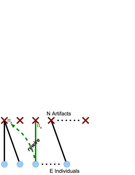
Figure 1: Illustration of the model.

The degree of the artifact vertices is $k$ indicating that one artifact has been ‘chosen’ by $k$ distinct individuals. The rewiring will be of the artifact ends of the edges, so each individual is always connected to the same edge. It is the degree distribution of the artifact vertices which we will consider so $n(k)$ is the number of artifacts each of which has been chosen by $k$ individuals. The probability distribution of interest is then $p(k)=n(k)/N$.

At each time step we make two choices but initially no changes to the network. First we choose an individual at random and consider its single link. This is equivalent to choosing an edge at random. It is also equivalent to picking an artifact vertex with pure preferential attachment, that is with probability proportional to its degree. We indicate the probability of choosing a particular artifact at this stage as $\Pi_{R}$ since we are going to remove this edge from this artifact.

The edge chosen is going to be attached to another artifact vertex picked with probability $\Pi_{A}$. This is the second choice we have to make and it will be done with a mixture of preferential attachment and random artifact vertex choice. In a fraction $p_{r}$ of the attachment events we chose a random artifact vertex to receive the rewired edge. In the context of studies of cultural transmission [16, 17, 18, 19, 20] this corresponds to innovation, while in gene evolution it is mutation [22]. Alternatively with probability $p_{p}$ we use preferential attachment to find a new artifact vertex for attachment. This is copying of the choice previously made by another individual, drift in the work on cultural transmission [16, 17, 18, 19, 20], while it is the inheritance mechanism in models of gene [22] or family name [21] homogeneity. If these are the only types of event $p_{p}+p_{r}=1$, the number of artifacts $N$ is constant and

$$\Pi_{R}=\frac{k}{E},\qquad\Pi_{A}=p_{r}\frac{1}{N}+p_{p}\frac{k}{E},\qquad(0\leq k\leq E)\;.$$ (1)

Note that there is a chance $\Pi_{R}\Pi_{A}$ that we will choose the same artifact vertex for both attachment and removal and there will then be no change in the network.

Finally, once both the artifacts for edge removal and addition have been picked, we perform the rewiring. The mean field equation for evolution of $n(k)$ is then [26]

$$n(k,t+1)-n(k,t)$$ (2)

$$= n(k+1,t)\Pi_{R}(k+1,t)\left(1-\Pi_{A}(k+1)\right)$$

$$-n(k,t)\Pi_{R}(k,t)\left(1-\Pi_{A}(k)\right)-n(k,t)\Pi_{A}(k,t)\left(1-\Pi_{R}(k)\right)$$

$$+n(k-1,t)\Pi_{A}(k-1,t)\left(1-\Pi_{R}(k-1)\right),\qquad(0\leq k\leq E)$$

We must set $n(k)=\Pi_{R}(k)=\Pi_{A}(k)=0$ for $k=-1$ and $k=E+1$ to ensure this equation is valid at the boundaries $k=0$ and $k=E$. It is crucial that we include the factors of $(1-\Pi_{A})$ and $(1-\Pi_{R})$ otherwise the behaviour at the boundaries is incorrect. We are explicitly excluding events where the same vertex is chosen for removal and attachment in any one rewiring event as they do not change the network but they are likely only if $n(k\sim E)=1$. Such $(1-\Pi)$ terms are missing from other discussions of such models but the literature usually has $n(k\sim E)\ll 1$ so these factors are negligible. Thus the results in the literature will be approximately the same as ours in this regime.

We can rephrase this as a Markov process. Consider a vector $\mathbf{n}(t)$ where $n_{i}(t)=n(E+1-i,t)$ for $i=1,2,\ldots,E+1$. Then we can think of the equations (2) as

$$\mathbf{n}(t+1) = {\mathbf{\textsf{M}}}\mathbf{n}(t).$$ (3)

The transition matrix is

M $$:= \begin{pmatrix}g(E)&h(E-1)&0&\cdots&&0&0\\ f(E)&g(E-1)&h(E-2)&&&&\\ 0&&\ddots&&&&\vdots\\ 0&&f(k+1)&g(k)&h(k-1)&&0\\ \vdots&&&\ddots&&&0\\ &&&&f(2)&g(1)&h(0)\\ 0&0&&\cdots&0&f(1)&g(0)\end{pmatrix}.$$ (4)

where the matrix entries are specified by the functions

$$f(k) = \Pi_{R}(k)(1-\Pi_{A}(k))$$ (5a)

$$g(k) = 1-f(k)-h(k)$$ (5b)

$$h(k) = \Pi_{A}(k)(1-\Pi_{R})$$ (5c)

The evolution is then given by the eigenvectors and eigenvalues of M

$$\mathbf{n}(t)=c_{1}\mathbf{e}^{(1)}+\sum_{i=2}^{E+1}c_{i}\lambda_{i}^{t}\mathbf{e}^{(i)}, 1=\lambda_{1}>\lambda_{2}\geq\ldots\geq|\lambda_{i}|\geq\lambda_{i+1}\geq\ldots$$ (6)

$${\mathbf{\textsf{M}}}\mathbf{e}^{(j)}=\lambda_{j}\mathbf{e}^{(j)} j=1,2,\ldots(E+1)$$ (7)

Stationary Solution

The stationary solution for the degree distribution $n(k,t)=n(k)$, the eigenvector associated with the largest eigenvalue $\lambda_{1}=1$, can be found by substituting $n(k,t)=n(k)$ into the evolution equation (2). We then note that if the first and third lines are equal then so are the second and third lines. Thus we look for solutions of the form

$$n(k+1)\Pi_{R}(k+1,t)\left(1-\Pi_{A}(k+1)\right)=n(k)\Pi_{A}(k,t)\left(1-\Pi_{R}(k)\right).$$ (8)

The result is [26]

$$n(k)=A^{(1)}\frac{\Gamma(k+\frac{p_{r}}{p_{p}}\langle k\rangle)}{\Gamma(k+1)}\frac{\Gamma(\frac{E}{p_{p}}-\frac{p_{r}}{p_{p}}\langle k\rangle-k)}{\Gamma(E+1-k)}\qquad(E\geq k\geq 0)$$ (9)

where $A$ is a constant normalisation and the average degree is $\langle k\rangle=E/N$. This solution has two characteristic parts. The first ratio of Gamma functions for $E\gg k\gg 1$ behaves as

$$\frac{\Gamma(k+\frac{p_{r}}{p_{p}}\langle k\rangle)}{\Gamma(k+1)}\propto k^{-\gamma}\left(1+O(k^{-1})\right),\qquad\gamma=1-\frac{p_{r}}{p_{p}}\langle k\rangle\leq 1\;.$$ (10)

For $p_{r}E=Np_{p}$ we have an exact inverse power law. The power is always below one but for many values ($p_{r}\ll 1$) the power is close to one. This is very different from the results for simple models with growth in the number of edges where demanding that the first moment is finite, $\langle k\rangle<\infty$, requires $\gamma>2$.

However the $(1-\Pi_{A})$ and $(1-\Pi_{R})$ terms in (2) have led to the second ratio of Gamma functions which if $p_{p}k\ll E$ gives an exponential cutoff

$$\frac{\Gamma\left(\frac{E}{p_{p}}-\frac{p_{r}}{p_{p}}\langle k\rangle-k\right)}{\Gamma(E+1-k)} \propto \exp\{-\zeta k\}(1+O(\frac{k}{E})),\qquad k\ll\left(\frac{E}{p_{p}}-\frac{p_{r}}{p_{p}}\right),$$ (11)

$$\zeta = -\ln\left(p_{p}\right)-\frac{2p_{r}\langle k\rangle}{E}$$ (12)

$$\approx p_{r}\mbox{ if }p_{r}\ll 1,\;\langle k\rangle\ll E\;.$$ (13)

However the numerator of this second ratio of Gamma functions becomes very large for $k=E$ if $(E-p_{r}\langle k\rangle)\ll p_{p}$. So this happens if $p_{r}\ll p_{r,\mathrm{simple}}$, where

$$p_{r,\mathrm{simple}}=\frac{1}{E+1-\langle k\rangle}\approx\frac{1}{E}+\frac{(\langle k\rangle-1)}{E^{2}}+O(E^{-2})\;.$$ (14)

This spike at $k=E$ will dominate the degree distribution. The point where the distribution has become flat at the upper boundary, so $n(E)=n(E-1)$ defines another critical random attachment probability $p_{r,\mathrm{crit}}$ at

$$p_{r\mathrm{crit}} = \frac{E-1}{E^{2}+E(1-\langle k\rangle)-1-\langle k\rangle}$$ (15)

$$Ep_{r\mathrm{crit}} \approx 1+\frac{(\langle k\rangle-2)}{E}$$ (16)

Thus when $p_{r}\lesssim 1/E$ the degree distribution will show a spike at $k=E$.

Overall we see two distinct types of distribution. For large innovation or mutation rates, $Ep_{r}\gtrsim 1$, we get a simple inverse power with an exponential cutoff

$$n(k)\propto(k)^{-\gamma}\exp\{-\zeta k\},\qquad p_{r}\gtrsim\frac{1}{E}$$ (17)

This is the behaviour noted in the literature [24, 22, 20, 18, 25] and since $Ep_{r}\gtrsim 1$ the formulae of the literature for the power $\gamma$ and cutoff $\zeta$ are a good approximation to the exact formulae given here. Note that in any one practical example it will be impossible to distinguish the power law derived from the data from $\gamma=1$. The power drifts away from one as we raise the innovation rate $p_{r}$ towards one but only at the expense of the exponential regime starting at lower and lower degree. That is, only when the power is very close to one can we get enough of a power law to be significant.

However as $p_{r}$ is lowered towards zero we get a change of behaviour in the exponential tail around $p_{r}E\approx 1$. First we find the exponential cutoff $\zeta^{-1}$ moves to larger and larger values, eventually becoming bigger than $E$. In fact this second ratio of Gamma functions becomes equal to one for all $k$ at $p_{r}=p_{r,\mathrm{simple}}\approx E^{-1}$. At that value of $p_{r}=p_{r,\mathrm{simple}}$ we have no cut off and we are closest to an exact inverse power law for all degree values. Slightly below that value of $p_{r}$ the tail starts to rise for $p_{r}>p_{r,\mathrm{crit}}\approx E^{-1}$. For $p_{r}E\ll 1$, i.e. if there has been no random artifact chosen after most edges have been rewired once, then we will almost certainly find one artifact linked to most of the individuals, $n(E)\approx 1$.

These exact results for the degree distribution are for the mean field equations. These are only approximations but because in these models there are no correlations between vertices, they should be excellent approximations. Simulations confirm this as Figures 2 and 3 show.

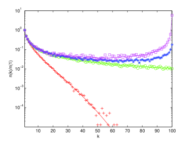
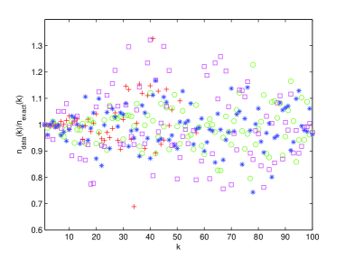
Figure 2: Plots of the degree distribution normalised with respect to $k=1$ and the fractional error of the data w.r.t. the exact solution. For $N=E=100$ and various $p_{r}=(1-p_{p})=0.1$ (crosses), $0.01$ (circles), $0.005$ (stars) and $0.001$ (squares), while lines are the exact solutions. Measured after $10^{5}$ rewiring events, averaged over $10^{4}$ runs. The size of fluctuations are clear from the deviations about the exact solutions.

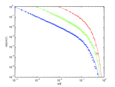
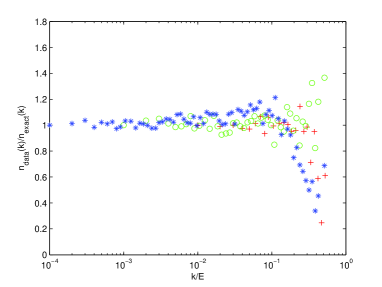
Figure 3: The degree distribution normalised to $n(1)$ and the fractional error w.r.t. the exact solution for $N=E$, $Ep_{r}=10.0$ and $p_{r}=10^{-2}$ (crosses), $10^{-3}$ (circles) and $10^{-4}$ (stars). Measured after $10^{7}$ rewiring events, averaged over $10^{3}$ runs. The tails of the distributions have few data points and so they show larger fluctuations about the the mean field results, as seen on the right. Despite this, for $p_{r}=10^{-4}$ there are clear signs we have not quite reached equilibrium. Started with $n(k=1)=E$ but otherwise zero.

The Generating Function

Given the exact solution for the degree distribution (9) its generating function $G(z)$, where

$$G(z):=\sum_{k=0}^{E}n(k)z^{k}\;,$$ (18)

is found to be

$$G(z) = n(0)F(\widetilde{K},-E;1+\widetilde{K}-E-\widetilde{E};z)$$ (20)

$$\widetilde{K}=\frac{p_{r}}{p_{p}}\langle k\rangle,\;\widetilde{E}=\frac{p_{r}}{p_{p}}E.$$

Here $F$ is the Hypergeometric function. The average fraction of sites of zero degree in the mean-field calculation is then exactly

$$\frac{n(0)}{N}=\frac{\Gamma(1-E-\widetilde{E})\Gamma(1+\widetilde{K}-\widetilde{E})}{\Gamma(1-E+\widetilde{K}-\widetilde{E})\Gamma(1-\widetilde{E})}.$$ (21)

The $m$-th derivative of the generating function is

$$\frac{1}{G(1)}\left.\frac{d^{m}G(z)}{dz^{m}}\right|_{z=1}\!=\langle k(k-1)\ldots(k-m+1)\rangle=\frac{\Gamma(\widetilde{K}+m)\Gamma(-E+m)\Gamma(1-\widetilde{E}-m)}{\Gamma(\widetilde{K})\Gamma(-E)\Gamma(1-\widetilde{E})}.$$ (22)

Knowing all the derivatives up to order $m$ gives all the moments $\langle k^{n}\rangle$ up to that order. For case $m=1$ this provides a consistency check on the parameter $\langle k\rangle=E/N$ - the average artifact degree.

New Artifact Addition

The cultural transmission models [16, 17, 19, 18, 20], the gene evolution model of [22] and the model of family name distributions [21] include another attachment process. There a new artifact vertex is added to the network with probability $\bar{p}=1-p_{r}-p_{p}$. The new artifact receives the edge removed from an existing artifact on the same time step. In this case the number of artifacts becomes infinite so most artifacts have no edges. Then the random attachment becomes completely equivalent to this new process of artifact addition. Thus the large $N$, zero $\langle k\rangle$ limit of our equations reproduces this case. The degree distribution for $k\geq 1$ behaves exactly as above — a simple inverse degree power law cutoff by an exponential for $E(1-p_{p})\gtrsim 1$ while for $E(1-p_{p})\lesssim 1$ $n(E)\approx 1$. In this model though, when $p_{r}=p_{r,\mathrm{simple}}$ we have a degree distribution which is an exact inverse power law for the whole range of non-zero degrees. Our exact solutions to the mean field equations again fits the data as Figure 4 shows.

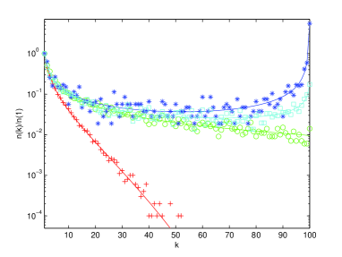
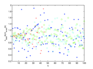
Figure 4: Plots of the degree distribution normalised with respect to $k=1$ and the fractional error of the data w.r.t. the exact solution. For $E=100$ but with new artifacts added with probability $p_{r}=0$, $\bar{p}=1-p_{p}$ where $\bar{p}=0.1$ (crosses), $0.01$ (circles), $0.005$ (squares) and $0.001$ (stars). The lines are the relevant exact mean field solutions. Measured after $10^{5}$ rewiring events, and averaged over $10^{4}$ runs.

Equilibration Rate

So far we have studied only the long time equilibrium distribution of (6) and therefore the first eigenvector of the matrix M of (4) associated with eigenvalue 1. However in Figure 3 there is clear evidence that the system has not yet reached equilibrium despite the apparently large number of rewiring events (each edge will have been rewired about $10^{4}$ times and results were averaged over 100 runs). This should be due to the second largest eigenvalue $\lambda_{2}$ in (6). We conjecture that this is of the form

$$\lambda_{2}=1-\frac{p_{r}}{E}\;.$$ (23)

We have shown that this is always an eigenvalue of the transition matrix M (4) and checked numerically that this is indeed the second largest eigenvalue for $E<100$. The eigenvector with this eigenvalue is

$$e^{(2)}_{E+1-k}=A^{(2)}\frac{\Gamma\left(k-\langle k\rangle+1\right)}{\Gamma\left(k-\langle k\rangle\right)}\frac{\Gamma\left(k+\frac{p_{r}}{(1-p_{r})}\langle k\rangle\right)}{\Gamma\left(k+1\right)}\frac{\Gamma\left(\frac{E}{(1-p_{r})}-\frac{p_{r}}{(1-p_{r})}\langle k\rangle-k\right)}{\Gamma\left(E+1-k\right)}\;.$$ (24)

This means that the equilibration time scale — the time taken for contributions from eigenvectors $\mathbf{e}^{(j)}$ ($j\geq 2$) to die away — is

$$\tau=-\frac{1}{\ln(\lambda^{(2)})}\approx\frac{E}{p_{r}}=\frac{E^{2}}{(p_{r}E)}$$ (25)

The parameter which controls the shape of the distribution for most examples is $(p_{r}E)$ and we expect to see the same shape independent of $E$. However what is noticable is that the rate of convergence slows as $E^{2}$ as we increase $E$ for fixed $p_{r}E$. This is visible in Figure 3. Figure 5 shows the results are consistent with our prediction in (25).

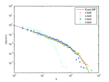
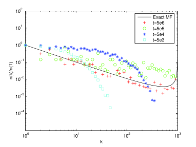
Figure 5: The degree distribution for $N=E=10^{3}$ for $(p_{r}E)=10$ (left) $(p_{r}E)=0.1$ (right), with $p_{p}=1-p_{r}$, $\bar{p}=0$, with the degree distribution taken at a variety of times: $5\times 10^{3}$ (squares), $5\times 10^{4}$ (stars), $5\times 10^{5}$ (circles) and $5\times 10^{6}$ (crosses). The initial configuration had each artifact connected to one individual and results were averaged over 100 runs. With $(p_{r}E)=10$ we are close to equilibrium after $t=5\times 10^{3}$ steps while this is only roughly true after $t=5\times 10^{5}$ time steps for $(p_{r}E)=0.1$, consistent with our prediction that the equilibration time scale is $\tau=E/p_{r}$.

Conclusions

We have analysed the degree distribution in rewiring network models and equivalent models which make no reference to a network. We have shown that the mean field equations are different from the ones considered in the literature. This makes little difference for results quoted when $p_{r}E\gg 1$ but we have demonstrated that only with the extra terms in (2) do we get the correct solution for all values of $p_{r}E$. Further we have found the second eigenvalue and its eigenvector and thus deduced the rate of convergence to the equilibrium solution. This scales as $E^{2}$ for fixed $p_{r}E$.

The literature suggests that probability distributions with a simple inverse size form plus a large scale cut off, as found in these models, are common. The real question is whether it is the copying mechanism which leads to such distributions in practice? It is difficult to understand why in the real world individuals choose a new artifact with a probability exactly equal to the number of times that artifact has been previously chosen, preferential attachment. It is known that for growing networks deviations from this law lead to deviations from power law distributions [28]. Surely in the real world, many decisions would be influenced by certain ‘leaders’ in their fields and we are more likely to copy their decision than that of other individuals?

In fact copying the choice of others, including that of certain ‘leaders’ may emerge naturally. Suppose our individuals were connected to each other by a second network, a ‘contacts’ network. Individuals could use their contacts by copying the advice of a friend or a friend of a friend as defined by the network of contacts. This is equivalent to making a finite length random walk on the graph of contacts. For growing networks this is known to be a way that the structure of the graph can self-organise into a scale-free form [11, 12, 13, 14] even if the random walk is only one step long. In a similar way, for non-growing networks, we are essentially making a one-step walk on the bipartite graph between individuals and artifacts, regardless of any network between the individuals. Extrapolating the results of [14] to the non-growing case suggests that this should be sufficient to generate an effective attachment probability of the form (1). Put simply we expect that whatever we do, the probability of arriving at one artifact at the end of a random walk is going to be dominated by the number of routes into that artifact, i.e. its degree.

Such an example may be seen in the the model of the minority game by Anghel et al. [23]. Their individuals are connected by a random graph and at each time step an individual copies the best strategy (the artifact in this case) from amongst the strategies of their neighbouring contacts. The individuals do not choose a random neighbour’s artifact but the ‘best’ artifact. However if the meaning of best is always changing, as it may be in the Minority Game or in many examples of fashion, this best choice may be effectively a random neighbour choice and hence be statistically equivalent to the simple copying used in our models. Thus even if it appears that the population is influenced by wise men or fashion leaders, provided there is little substance to their choices then it may well be equivalent to simple copying of one person’s choice. It should come as no surprise that the results for the artifact degree distribution in [23], the popularity of the most popular strategies, follows a simple inverse power law with a large degree cutoff, exactly as the simple copying model would give.

Finally one might ask if it is important to get the right classification of artifacts to see the distribution. What if people make choices based on one classification but we measure on another? Do people choose a specific breed of dog as registered by the dog breeders association of their country, or do they really choose between small and large dogs, short or long haired dogs [20]? The classification of pottery in archaeology is one imposed on the record by modern archaeologists. The answer ought to be that the classification should not be important and it is a scaling property of the model and its solutions that this is so.

Suppose we randomly paired all the artifacts but deemed the fundamental process to be based still on the choice of the original artifacts and their degree. The choice of edge to remove is unchanged while preferential attachment to the underlying individual artifacts leads to effective preferential attachment to the artifact pairs. The probability of an innovation event ($p_{r}$ or $\bar{p}$) is unchanged but the probability of choosing a random artifact pair is double that of choosing a single artifact. However that reflects the fact that the number of artifacts pairs $N_{2}$ is half the original number of artifacts. Thus we see that we require that $N\rightarrow N_{2}=(N/2)$ but we keep all other parameters the same. In particular the linear nature of preferential removal and attachment to the artifact pairs means that the form of both removal and attachment is unchanged. Overall we have exactly the same equations for the artifact pair degree distribution $n_{2}(k)$ as we did for the original artifacts. Thus the distribution $n(k)$ of (9) is of the same form with $N\rightarrow(N/2)$ being the only change required. However we have seen that for $Ep_{r}\gtrsim 1$ the shape can be parameterised in terms of a power $\gamma$ (10) and an exponential cutoff $\zeta$ (12). The latter is unchanged and while the power does change a little, we have argued that if $\gamma$ can be measured, it is likely to be indistinguishable from one in any real data set. So apart from the overall normalisation, the distribution of artifact choice is essentially independent of how we choose to classify the artifacts. This stability against the classification of the artifact types is an important feature of the copying models considered here.

TSE would like to thank H.Morgan and W.Swanell for useful discussions.

Supplementary Material

This plot is not in the published version.

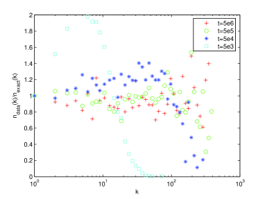
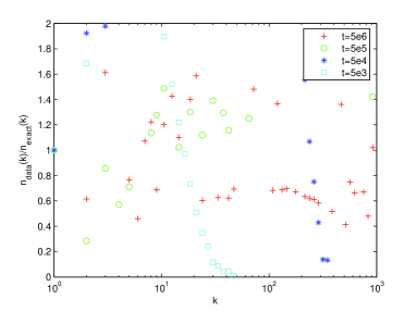
Figure 6: Plots of the fractional error of the data of Fig. 5 w.r.t. the exact solution for $(p_{r}E)=10$ (left) $(p_{r}E)=0.1$ (right). With $N=E=10^{3}$, $p_{p}=1-p_{r}$, $\bar{p}=0$, with the degree distribution taken at a variety of times: $5\times 10^{3}$ (squares), $5\times 10^{4}$ (stars), $5\times 10^{5}$ (circles) and $5\times 10^{6}$ (crosses). The initial configuration had each artifact connected to one individual and results were averaged over 100 runs. With $(p_{r}E)=10$ we are close to equilibrium after $t=5\times 10^{3}$ steps while this is only roughly true after $t=5\times 10^{5}$ time steps for $(p_{r}E)=0.1$, consistent with our prediction that the equilibration time scale is $\tau=E/p_{r}$.

References

- [1] G.U.Yule, “A Mathematical theory of evolution, based on the conclusions of Dr J.C.Willis, F.R.S.”, Phil.Trans.B.213 (1924) 21.
- [2] G.K.Zipf, “Human Behavior and the Principle of Least Effort” (Addison-Wesley, 1949).
- [3] H.A.Simon, “On a Class of Skew Distribution Functions”, Biometrika 42 (1955) 425.
- [4] D.J.de S.Price, “Networks of Scientific Papers”, Science 149 (1965) 510-515.
- [5] D.J.de S.Price, “A general theory of bibliometric and other cumulative advantage processes”, J.Amer.Soc.Inform.Sci. 27 (1976) 292-306.
- [6] H.J.Jensen, “Self-Organized Criticality” (CUP, Cambridge, 1998).
- [7] Thomas Hobbes, “The Leviathan” (1651).
- [8] A.-L.Barabási and R.Albert, “Emergence of scaling in random networks”, Science 286 (1999) 173 [cond-mat/9910332].
- [9] A.-L.Barabási, R.Albert and H.Jeong, “Mean-field theory for scale-free random networks”, Physica A 272 (1999) 173 [cond-mat/9907068].
- [10] T.S.Evans, “Complex networks”, Contemporary Physics 45 (2004) 455.
- [11] A.Vázquez, “Knowing a network by walking on it: emergence of scaling”, cond-mat/0006132.
- [12] A.Vázquez, “Growing networks with local rules: preferential attachment, clustering hierarchy and degree correlations”, Phys. Rev.E 67 (2003) 056104 [cond-mat/0211528].
- [13] J.Saramäki and K.Kaski, “Scale-Free Networks Generated by Random Walkers”, Physica A 341 (2004) 80 [cond-mat/0404088].
- [14] T.S.Evans and J.P.Saramäki, “Scale Free Networks from Self-Organisation”, Phys.Rev.E 72 (2005) 026138 [cond-mat/0411390].
- [15] D.J.Watts and S.H.Strogatz, “Collective dynamics of ‘small-world’ networks”, Nature 393 (1998) 440.
- [16] F.D.Neiman, “Stylistic variation in evolutionary perspective: Inferences from decorative diversity and inter-assemblage distance in Illinois Woodland Ceramic assemblages”, American Antiquity 60 (1995) 1-37.
- [17] R.A.Bentley and S.J.Shennan, “Cultural Transmission and Stochastic Network Growth”, American Antiquity 68 (2003) 459-485.
- [18] R.A.Bentley, M.W.Hahn and S.J.Shennan, “Random Drift and Cultural Change”, Proc.R.Soc.Lon.B271 (2004) 1443-1450.
- [19] M.W.Hahn and R.A.Bentley, “Drift as a Mechanism for Cultural Change: an example from baby names”, Proc.R.Soc.Lon.B270 (2003) S120-S123.
- [20] H.A.Herzog, R.A.Bentley and M.W.Hahn, “Random drift and large shifts in popularity of dog breeds”, Proc.R.Soc.Lon B (Suppl.) 271 (2004) S353-S356.
- [21] D.Zanette and S.Manrubia, “Vertical transmission of culture and the distribiution of family names”, Physica A 295 (2001) 1 [nlin.AO/0009046].
- [22] M.Kimura and J.F.Crow, “The Number of Alleles that can be Maintained in a Finite Population”, Genetics 49 (1964) 725-738.
- [23] M.Anghel, Z.Toroczkai, K.E.Bassler and G.Korniss, “Competition in Social Networks: Emergence of a Scale-Free Leadership Structure and Collective Efficiency”, Phys.Rev.Lett 92 (2004) 058701.
- [24] K.Park, Y.-C.Lai and N.Ye, “Self-organized scale-free networks”, Phys.Rev.E72 (2005) 026131.
- [25] Y.-B.Xie, T.Zhou and B-.H.Wang, “Scale-free networks without growth”, cond-mat/0512485.
- [26] T.S.Evans, “Exact Solutions for Network Rewiring Models”, cond-mat/0607196.
- [27] T.S.Evans and A.D.K.Plato (in preparation).
- [28] P.L.Krapivsky, S.Redner and F.Leyvraz, “Connectivity of Growing Random Networks”, Phys.Rev.Lett. 85 (2000) 4629[cond-mat/0005139].