Dynamics of a viscous vesicle in linear flows

Abstract

An analytical theory is developed to describe the dynamics of a closed lipid bilayer membrane (vesicle) freely suspended in a general linear flow. Considering a nearly spherical shape, the solution to the creeping–flow equations is obtained as a regular perturbation expansion in the excess area. The analysis takes into account the membrane fluidity, incompressibility and resistance to bending. The constraint for a fixed total area leads to a non–linear shape evolution equation at leading order. As a result two regimes of vesicle behavior, tank–treading and tumbling, are predicted depending on the viscosity contrast between interior and exterior fluid. Below a critical viscosity contrast, which depends on the excess area, the vesicle deforms into a tank–treading ellipsoid, whose orientation angle with respect to the flow direction is independent of the membrane bending rigidity. In the tumbling regime, the vesicle exhibits periodic shape deformations with a frequency that increases with the viscosity contrast. Non-Newtonian rheology such as normal stresses is predicted for a dilute suspension of vesicles. The theory is in good agreement with published experimental data for vesicle behavior in simple shear flow.

I Introduction

The dynamics of deformable particles such as drops, capsules and cells in flow represents a long–standing problem of interest in many branches of science and engineering, for instance because of its relevance to the rheology of emulsions and biological suspensions such as blood. The problem is challenging because the shape of these “soft” particles is not given a priori but is governed by the balance between interfacial forces, e.g. due to stretching and/or bending of the interface, and fluid stresses. The interfacial properties, therefore, play a crucial role in the dynamics of these particles.

The interface between two simple fluids is governed by the surface tension, which is isotropic, in the absence of surfactants or heating. Surface tension acts to minimize the interfacial area; therefore the rest shape of a drop is a sphere. Under shear flow, the drop deforms initially into an ellipsoid. As the flow strength increases, the drop area also increases and the angle between the ellipsoid major axis and flow direction decreases from $\pi/4$. If the flow strength is sufficiently high, and the viscosity contrast is moderate, the drop breaks up. Drop microhydrodynamics has been studied quite extensively Rallison (1984); Stone (1994).

Polymerized membrane interfaces found in synthetic capsules and the red blood cell, where a lipid bilayer is attached to a scaffolding of cytoskeletal proteins, exhibit far more complicated mechanical properties. These membranes behave as thin viscoelastic materials that can develop bending moments similar to thin elastic shells. Barthes-Biesel Barthes-Biesel (1991) has reviewed the various constitutive laws adopted to describe the membrane mechanics and the effects of interfacial properties on the capsule behavior in a linear flow. Yet, most of the theoretical studies treat the membrane as a two–dimensional viscoelastic surface with no bending resistance.

Bending stiffness, however, plays a crucial role in the mechanics of biological membranes, for example the equilibrium biconcave shape of the red blood cell can not be accounted for without including bending resistanceCanham (1970). The main structural component of the cell membrane is the lipid bilayer and its mechanical properties are essential to the overall cell mechanics. The pure lipid membrane consists of two sheets of lipid molecules. The molecular thickness imparts bending resistance. Lipid molecules are free to move within the monolayer, and therefore, in contrast to solid–like polymerized membranes, the lipid bilayer membrane is fluid. In addition, since the lipid bilayer contains a fixed number of molecules with fixed area per molecule (under moderate stresses), the membrane is incompressible and the total area is constant. The enclosed volume is also constant at given osmotic conditions. The mechanics of lipid bilayers in concisely reviewed in PowersPowers (2005).

Equilibrium mechanical properties of vesicles made of lipid bilayer membranes are fairly well understood Seifert (1997), and vesicle shapes can be generated by minimizing the membrane bending energy subject to the constraints of constant area and enclosed volume. In contrast, the non–equilibrium dynamics of lipid bilayer membranes has been studied only to a limited extent. Experimental studies de Haas et al. (1997); Kantsler and Steinberg (2005, 2006); Mader et al. (2006) of vesicle behavior in unbounded shear flow observe that in weak flows, and when the inner and outer fluids are the same, the vesicle deforms into a tank-treading stationary prolate ellipsoid with an inclination angle close to $\pi/4$ with respect to the flow direction; however, in striking contrast to drops, when the fluid inside is more viscous than outside the vesicle undergoes a tumbling motion. Numerical simulations Kraus et al. (1996); Beaucourt et al. (2004); Noguchi and Gompper (2004) and analytical theoriesSeifert (1999a); Olla (2000); Misbah (2006) of vesicle microhydrodynamics attempt to elucidate such experimental observations. In their classic paper Keller and SkalakKeller and Skalak (1982) analyzed the motion of a tank–treading ellipsoid in unbounded shear flow. The theory qualitatively captures features like the tumbling transition, but their assumption of a fixed particle shape casts some doubts on the applicability to deformable vesicles; for instance, no connection can be made to the physical properties of real membranes such as the bending rigidity. The free-boundary character of the problem is taken into account in several recent works. Shape evolution of a fluctuating quasi–spherical vesicle was considered by SeifertSeifert (1999a) for the case where the inner and suspending fluids are the same, i.e. there is no viscosity contrast. The theory predicts a stationary, tank–treading prolate ellipsoid and no transition to tumbling motion. The importance of viscosity contrast for the tumbling transition was recognized by MisbahMisbah (2006), who showed quantitatively that a critical value of viscosity contrast exists which separates the tank–treading and tumbling regimes. The critical viscosity ratio was shown to decrease with the excess area (the difference in the areas of the vesicle and an equivalent sphere with the same volume). He also pointed out that the area constraint leads to non-linear leading order evolution equations for the vesicle shape, which in the case when only ellipsoidal deformation modes are considered are independent of the membrane bending rigidity. Earlier work by OllaOlla (2000) derived similar results for a viscoelastic membrane.

Cell behavior in unbounded flow is of fundamental interest. However, flows in confined geometries are much more relevant to physiology, for instance blood flow in the microcirculation. Walls affect greatly particle microhydrodynamics, for example red blood cells migrate away from the blood vessel walls, an observation that dates back to Poiseuille Sutera and Skalak (1993). The existence of a near–wall cell–depleted region accounts for the Fahraeus–Lindqvist effect, which is the decrease of the apparent blood viscosity in smaller vesselsPopel and Johnson (2005). Cell traffic between the blood stream and tissues involves cell attachment to blood vessel walls Orsello et al. (2001); examples are leukocytes during inflammatory response, platelets in formation of atherosclerotic plaques, or tumor cells in metastasis. In order to elucidate the fundamental features of the process, several studies have used vesicles as the simplest artificial cell Lorz et al. (2000); Abkarian et al. (2002); Abkarian and Viallat (2005). They have reported that the flow–induced deformation of adhering vesicles gives rise to a lift force that can lead to unbinding from the substrate. The experimental data on the lift force and vesicle migration velocity have not yet been quantitatively compared to theoretical studies Cantat and Misbah (1999); Sukumaran and Seifert (2001); Seifert (1999b).

The purpose of this paper is to simultaneously include the effects of (i) viscosity contrast, (ii) membrane incompressibility and (iii) bending rigidity in the analysis of vesicle dynamics in shear flows, unbounded or in the presence of a wall, in a consistent way and thereby proceed further towards a fully quantitative description of the experimentally observed vesicle behavior. As a first step, the leading order small deformation of a nearly–spherical vesicle will be considered. However, the developed formalism will serve as a rigorous basis for considering higher orders in the non–linear dynamics of a vesicle in flow.

Our study extends the results of SeifertSeifert (1999a) derived for an equiviscous vesicle. The works by MisbahMisbah (2006) and OllaOlla (2000) are clarified, more specifically, the calculations are presented more explicitly, some important results are corrected and cast in a form that can be directly compared to experimental measurements, and more physical insights are given for the vesicle behavior in the tumbling regime. We demonstrate that the theory agrees quantitatively with published experimental dataKantsler and Steinberg (2005, 2006); Mader et al. (2006). We present new results for (i) the non–Newtonian rheology of a vesicle suspension, in particular, we show how the single vesicle solution serves to calculate the effective stress of a collection of many vesicles and we predict the existence of normal stresses, and (ii) vesicle migration velocity in wall-bounded flow in the case of large distances from the boundary.

II Problem formulation

Let us consider a neutrally–buoyant vesicle formed by a closed lipid bilayer membrane with total area $A$. The vesicle is suspended in a fluid of viscosity $\eta$ and filled with a fluid of viscosity $\left({\lambda}-1\right)\eta$ . Both interior and exterior fluids are incompressible and Newtonian. The vesicle has a characteristic size $a$ defined by the radius of a sphere of the same volume. The equilibrium shape of the vesicle is characterized by a small excess area

$$\Delta=A/a^{2}-4\pi\,.$$ (1)

The coordinate system employed is spherical $(r,\,\theta,\,\phi)$, with the origin coinciding with the center of mass of the vesicle. The interface is specified by a shape function $F\left({\bf r},t\right)$, of the position ${\bf r}$ and time $t$, which represents the interface as the set of points, where $F\left({\bf r},t\right)\equiv 0$. It is given by the relation

$$F\left({\bf r},t\right)=r-r_{\mathrm{s}}\left(\theta,\phi,t\right)\,.$$ (2)

II.1 Hydrodynamics

The vesicle is placed in a steady two-dimensional linear flow

$${\bf v}^{\infty}({\bf r})=\dot{\gamma}{\bf E}\cdot{\bf r},$$ (3)

where $\dot{\gamma}$ is the strain rate, and ${\bf E}$ is the velocity gradient tensor. Linear flows are defined by

$${\bf E}={\frac{1}{2}}\left(\begin{array}[]{ccc}0&1+\omega&0\\ 1-\omega&0&0\\ 0&0&0\end{array}\right),$$ (4)

where $\omega$ is the magnitude of the rotational flow component. Irrotational flow such as the pure extensional flow is given by $\omega=0$. Simple shear flow is specified by $\omega=1$, i.e. $v^{\infty}_{x}=\dot{\gamma}y$. A sketch of the problem is shown in Figure 1.

Figure 1: A sketch of a vesicle is a simple shear flow. The zoomed region of the interface illustrates the bilayer lipid structure of the membrane.

Typically vesicles are micron-sized. At these small length-scales water is effectively very viscous, inertial effects are unimportant and fluid velocity fields inside ${\bf v}^{{\mathrm{in}}}$ and outside ${\bf v}^{{\mathrm{out}}}$ the vesicle are described by the Stokes equations

$$\begin{split}\eta\nabla^{2}{\bf v}^{\mathrm{out}}-\bm{\nabla}p^{\mathrm{out}}=0,&\quad\bm{\nabla}\cdot{\bf v}^{\mathrm{out}}=0\,,\\ ({\lambda}-1)\eta\nabla^{2}{\bf v}^{\mathrm{in}}-\bm{\nabla}p^{\mathrm{in}}=0,&\quad\bm{\nabla}\cdot{\bf v}^{\mathrm{in}}=0\,.\end{split}$$ (5)

Far away from the vesicle, the flow field tends to the unperturbed external flow ${\bf v}^{{\mathrm{out}}}\rightarrow{\bf v}^{\infty}$. Velocity is continuous across the interface

$${\bf v}^{{\mathrm{in}}}={\bf v}^{{\mathrm{out}}}\equiv{\bf v}_{s}\quad\mbox{at}\,\quad r=r_{s}\,,$$ (6)

where $r_{\mathrm{s}}$ denotes the position of the interface. The interface moves with the fluid velocity Leal (1992)

$$\frac{\partial F}{\partial t}+{\bf v}_{\mathrm{s}}\cdot\bm{\nabla}F=0\,,$$ (7)

where ${\bf v}_{\mathrm{s}}$ is the fluid velocity at the vesicle interface. Fluid motion gives rise to bulk hydrodynamic stress

$${\bf T}=\textstyle-p{\bf I}+\eta(\bm{\nabla}{\bf u}+(\bm{\nabla}{\bf u})^{T})\,,$$ (8)

where ${\bf I}$ denotes the unit tensor and the superscript ${\it T}$ denotes transpose. The surrounding fluids exert tractions on the membrane that are balanced by membrane forces

$${\bf n}\cdot\left({\bf T}^{\mathrm{out}}-{\bf T}^{\mathrm{in}}\right)={\bf t}^{\mathrm{mem}}\quad\mbox{at}\,\quad r=r_{s}\,$$ (9)

where ${\bf n}$ is the outward unit normal vector and the membrane surface forces are discussed next.

II.2 Membrane mechanics

Unlike drops, which are governed by surface tension, the shape of the vesicle is determined by bending elasticitySeifert (1997). A nonequilibrium membrane configuration gives rise to a surface force densitySeifert (1999a)

$$\begin{split}{\bf t}^{\mathrm{mem}}=&\left[2\sigma H-\kappa\left(4H^{3}-4KH+2\nabla_{s}^{2}H\right)\right]{\bf n}\\ &-\bm{\nabla}_{s}\sigma\,,\end{split}$$ (10)

where $\kappa$ is the bending rigidity, $H$ and $K$ are the mean and Gaussian curvatures, respectively, and $\sigma$ is the local membrane tension. The tangential part of the surface force density arises from nonuniformities in the surface tension, which are needed to ensure local area incompressibility, as discussed in more details in the next section. The mean and Gaussian curvatures are

$$H=\frac{1}{2}\bm{\nabla}\cdot{\bf n}\,,$$ (11)

$$K=\frac{1}{2}\bm{\nabla}\cdot\left({\bf n}\bm{\nabla}\cdot{\bf n}+{\bf n}\times\left(\bm{\nabla}\times{\bf n}\right)\right)\,,$$ (12)

where the outward unit normal vector can be determined from the shape function (2) via

$${\bf n}=\frac{\bm{\nabla}F}{|\bm{\nabla}F|}\,.$$ (13)

The surface gradient operator is defined as

$$\bm{\nabla}_{\mathrm{s}}={\bf I}_{\mathrm{s}}\cdot\bm{\nabla}\,,$$ (14)

where the matrix ${\bf I}_{\mathrm{s}}={\bf I}-{\bf n}{\bf n}$ represents a surface projection. At rest, Eq. (9) reduces to the well–known Euler–Lagrange equation

$$p^{\mathrm{in}}-p^{\mathrm{out}}=2\sigma H-\kappa\left[4H^{3}-4KH+2\nabla_{s}^{2}H\right]\,.$$ (15)

II.3 Area constraint and tension

The lipid bilayer is fluid because the lipids can diffuse rapidly within the membrane. Moreover, since the number of lipids in a monolayer and the area per lipid are fixed, the lipid bilayer membrane is incompressible and the total area is conserved. A membrane element only deforms but does not change its area. Accordingly, the local tension changes in order to keep the local area constant. Hence, inhomogeneities in the tension ensure local area incompressibility. The situation is analogous to three–dimensional incompressible fluids, where finite changes in pressure (tension is the two-dimensional analogue) correspond to infinitesimal changes in fluid density, and pressure takes the place of the density as an independent field variable; in flowing fluids pressure can become nonuniform. The local area conservation implies that the velocity field at the interface is solenoidalSeifert (1999a)

$$\bm{\nabla}_{s}\cdot{\bf v}=0\,.$$ (16)

The global area constraint acts like an isotropic tension whose value at equilibrium is given by the Lagrange multiplier used to determine the shapeSeifert (1995). Under flow, the changes in shape result in variations of this effective isotropic tension.

II.4 Dimensionless parameters

Viscous forces exerted by the extensional component of the external flow drive shape deformation that occurs on a time scale

$$t_{\mathrm{\dot{\gamma}}}={\lambda}\dot{\gamma}^{-1}\,.$$ (17)

Several intrinsic relaxation mechanisms oppose the deformation. Bending stresses work to bring the shape back to its preferred curvature state; the corresponding time scale is

$$t_{\kappa}=\frac{{\lambda}\eta a^{3}}{\kappa}\,.$$ (18)

In shear flow, vesicle rotation away from the extensional axis of the imposed flow effectively decreases the extent of shape distortion; the associated time scale is

$$t_{\mathrm{r}}=\dot{\gamma}^{-1}.$$ (19)

The strength of these two relaxation mechanisms that limit shape deformation by the flow is quantified by the corresponding dimensionless parameters: the capillary number

$$\chi=\frac{t_{\kappa}}{t_{\mathrm{\dot{\gamma}}}},$$ (20)

and the rotation parameter

$$\frac{t_{\mathrm{r}}}{t_{\mathrm{\dot{\gamma}}}}={\lambda}^{-1}.$$ (21)

The smaller of these parameters controls the magnitude of vesicle deformation. At moderate viscosity ratios, the vesicle shape should remain close to the equilibrium one provided that the capillary number is small, i.e. restoring bending forces are stronger than the distorting viscous forces. A high viscosity inner fluid limits the shape distortion in flows with non-zero vorticity by means of increasing the rate of vesicle rotation. In addition to the flow–related parameters, a physical parameter that arises from vesicle geometry is the excess area (1), which sets the maximum magnitude of the shape distortion; it turns out to be the relevant small parameter for the analysis of nearly–spherical vesicles as shown in the next sections.

Henceforth, bending stresses and tension are normalized by $\kappa/a^{2}$; all other quantities are rescaled using $\eta$, $a$, and $\dot{\gamma}$. Accordingly, the time scale is $\dot{\gamma}^{-1}$, the velocity scale is $\dot{\gamma}a$, bulk stresses are scaled with $\eta\dot{\gamma}$.

III Small deformation theory

In this section we present a perturbative solution for the microhydrodynamics of a vesicle with a nearly spherical shape.

In the coordinate system centered at the vesicle, the radial position $r_{\mathrm{s}}$ of the vesicle interface can be represented as

$$r_{\mathrm{s}}=\alpha+f\left(\Omega\right)\,,$$ (22)

where $f$ is the deviation of vesicle shape from a sphere, which depends only on the angles ($\theta\,,\phi$) (or equivalently the solid angle $\Omega$) and has a vanishing angular average

$$\int f\,{\mathrm{d}}{\Omega}=0\,.$$ (23)

The isotropic contribution $\alpha$ is determined by the volume-conservation constraint

$$\int(\alpha+f)^{3}\,{\mathrm{d}}{\Omega}=4\pi\,.$$ (24)

The total area conservation constraint relates the amplitude of the perturbation $f$ and the excess area $\Delta$

$$A/a^{2}=\int\frac{r_{s}^{2}}{\hat{\bf r}\cdot{\bf n}}d\Omega=4\pi+\Delta\,.$$ (25)

where $\hat{\bf r}$ denotes the unit radial vector.

III.1 Expansion in spherical harmonics

In Eq. (22), the function $f$ representing the perturbations of the vesicle shape depends only on angular coordinates. Thus, it is expanded into series of scalar spherical harmonics $Y_{jm}$ (54)

$$f=\sum_{j=2}^{\infty}\sum_{m=-j}^{j}f_{jm}Y_{jm}\,,$$ (26)

In the above equation, the summation starts from nonzero $j$ because $f$ includes only the nonisotropic contributions. For small shape perturbations around a sphere the volume constraint (24) becomesSeifert (1999a); Vlahovska et al. (2005)

$$\alpha=1-\frac{1}{4\pi}\sum_{jm}f_{jm}f^{*}_{jm}+O(f^{3})\,,$$ (27)

where the sum over $j$ starts from 2, $|m|\leq j$ and $f^{*}_{jm}=(-1)^{m}f_{j-m}$. Similarly, the area constraint (25) transforms to

$$\Delta=\sum_{jm}a(j)f_{jm}f^{*}_{jm}+O(f^{3})\,,$$ (28a)

where

$$a(j)=\frac{\left(j+2\right)\left(j-1\right)}{2}\,.$$ (28b)

The tension is expanded in scalar spherical harmonics

$$\sigma=\sigma_{0}+\sum_{j=2}^{\infty}\sum_{m=-j}^{j}\sigma_{jm}Y_{jm}\,,$$ (29)

where $\sigma_{0}$ is the isotropic part of the tension, which varies with shape in order to keep the total area constant. It is determined from the condition that the modes must satisfy the area constraint $\dot{\Delta}=0$, i.e.

$$\sum_{jm}a_{j}\dot{f}_{jm}f^{*}_{jm}=0\,.$$ (30)

The nonuniform part of the tension is related to the local incompressibility.

III.2 Perturbation solution

The combination of perturbative analysis and the spherical harmonics formalism for solving Stokes-flow problems involving a deformable particle has been developed in detail in Vlahovska et al. Vlahovska (2003); Vlahovska et al. (2005) for the problem of a surfactant–covered drop. Here we present a brief outline of the method, and focus on the new feature specific to lipid bilayer membranes which is the area constraint.

This paper considers a non–spherical particle albeit the shape deviation from sphericity is small, i.e. $f\sim O({\varepsilon})$ and ${\varepsilon}\ll 1$. In this case, the exact position of the interface is replaced by the surface of a sphere of equivalent volume, and all quantities that are to be evaluated at the interface of the deformed particle are approximated using a Taylor series expansion.

III.2.1 Small parameter for area-constrained dynamics

Small deformations of initially spherical drops and capsules with elastic membranes have been considered in a number of studies Barthès-Biesel and Acrivos (1973); Barthes-Biesel (1980). Typical choices for the small parameter are the capillary number or the inverse viscosity ratio.

In contrast to drops and capsules, the rest shape of the vesicle we consider is non–spherical. The excess area plays a crucial role in the vesicle dynamics, because under the constraints of constant area and volume a sphere is a geometrically rigid object. Consequently, in the absence of excess area, a vesicle behaves as a rigid sphere.

Thus, the appropriate small parameter that reflects the importance of the excess area in the vesicle dynamics is

$${\varepsilon}=\Delta^{{\frac{1}{2}}}\,.$$ (31)

The square root comes from the observation that $f^{2}\sim\Delta$ (28). The choice of the excess area as the small parameter allows vesicle behavior to described, where the whole excess area is involved in the vesicle deformation.

III.2.2 Evolution equation

We solve the hydrodynamic problem to obtain the velocity field, and use the fact that the interface moves with the normal component of the velocity to determine the shape evolution. The solution for small deviations from a sphere is presented in details in Appendix E. In this section we present the general expression for the shape evolution equation valid for any linear flow. In the subsequent sections we analyze in more details the particular case of simple shear flow.

At leading order the evolution of the shape parameters (26) is described by

$$\dot{f}_{jm}={\mathrm{i}}\omega\frac{m}{2}f_{jm}+{\lambda}^{-1}C({\lambda},j,m)+{\lambda}^{-1}\chi^{-1}\Gamma\left({\lambda},\sigma_{0},j\right)f_{jm}+O\left({\lambda}^{-1}{\varepsilon},{\varepsilon}^{2}\right)\,,$$ (32)

where the isotropic tension $\sigma_{0}$ is determined using the area constraint (28) as described in Appendix F, see Eq. (89). The first term in the evolution equation (32) describes rigid body rotation of a particle with shape $f$ by the rotational component of the external flow. The second term describes the distortion of the vesicle shape by the extensional component of the external flow. The term including $\chi$ is associated with relaxation driven by the membrane stresses. The expressions for $C$ and $\Gamma$ are given by (80). These coefficients depend on ${\lambda}$ and are bounded at ${\lambda}\rightarrow\infty$.

The area constraint couples all modes, and results in isotropic tension, which depends nonlinearly on the shape. Thus the leading order vesicle dynamics is non–linear in contrast to the corresponding results for drops and capsules. As we show in the next section, a peculiar consequence from the area–constrained dynamics is that the stationary solution is independent of the capillary number.

IV Results: Simple shear flow

In this section we provide analytical solutions for the vesicle shape evolution in a simple shear flow. Simple shear flow consists of an extensional component, ${\bf v}^{\infty}_{ext}={\frac{1}{2}}(y,x,0)$ , which in the spherical harmonics representation (63) is described by

$$\textstyle c^{\infty}_{2\pm 20}=\mp{\mathrm{i}}\sqrt{\frac{\pi}{5}}\,\quad c^{\infty}_{2\pm 22}=\mp{\mathrm{i}}\sqrt{\frac{2\pi}{15}}\,,$$ (33a)

and a rotational component, $${\bf v}^{\infty}_{rot}={\frac{1}{2}}(y,-x,0)$$, which is specified by

$$\textstyle c^{\infty}_{101}={\mathrm{i}}\sqrt{\frac{2\pi}{3}}\,.$$ (33b)

The extensional part of external flow (3), which is responsible for shape distortion, is fully characterized by a second-order traceless tensor, which corresponds to spherical harmonics of the order $j=2$ (33a). Therefore, at leading order the shear flow affects only the subspace $j=2$. Considering only these modes simplifies the expression for the tension (89) and the evolution equations (32) to the following set of coupled non–linear differential equations

$$\begin{split}\dot{f}_{2m}=&\textstyle-\frac{{\mathrm{i}}m}{2}h({\lambda})\delta_{|m|2}+\frac{{\mathrm{i}}m}{2}f_{2m}\\ &-2{\mathrm{i}}h({\lambda})\Delta^{-1}(f_{22}-f_{2-2})f_{2-m}\end{split}$$ (34)

where

$$h({\lambda})=\frac{4\sqrt{30\pi}}{23{\lambda}+9}\,.$$ (35)

Strictly speaking Eq. (34) is only valid at long times ($t\gg t_{\kappa}$) when all transient $j\neq 2$ modes have decayed. The initial conditions are set by the equilibrium vesicle configuration. For example, for a fluctuating quasi–spherical vesicle Seifert (1999a)

$$|f_{jm}|^{2}=\frac{k_{B}T}{\kappa E(j,\sigma_{\mathrm{eq}})}\,,$$ (36)

where $E(j,\sigma)$ is given by (80d).

The shape parameters (26) are decomposed into real and imaginary parts

$$f_{jm}=f^{\prime}_{jm}+{\mathrm{i}}f^{\prime\prime}_{jm}\,\,\quad f^{*}_{jm}=f^{\prime}_{jm}-{\mathrm{i}}f^{\prime\prime}_{jm}$$ (37)

In the flow plane $x-y$, the vesicle shape $f$ is characterized by only three components, $f^{\prime}_{22}$ ,$f^{\prime\prime}_{22}$ , and $f_{20}$, corresponding to deformation along the flow axis $x$, straining axis $x=y$, and the $z$ axis. Shape modes $f_{2\pm 1}$ describe deformations of the type $xz$ and $yz$, which vanish in the flow plane $z=0$. From geometrical considerations we have for the inclination angle

$$\phi_{0}=-\frac{1}{2}\arctan\left(\frac{f_{22}^{\prime\prime}}{f_{22}^{\prime}}\right)\,.$$ (38)

IV.1 Tank–treading

The evolution equations (34) have two sets of stationary points. The first one corresponds to the tank–treading state. The only non–zero stationary amplitudes are

$$f_{22}^{\prime\prime}=-\frac{\Delta}{4h({\lambda})}\sqrt{-1+\frac{4h^{2}({\lambda})}{\Delta}}\,,\quad f_{22}^{\prime}=\frac{\Delta}{4h({\lambda})}\,.$$ (39)

The numerical solution of the full set of evolution equations (32) shows that all other modes decay to zero. Hence, in the stationary state all excess area is stored in the $f_{2\pm 2}$ modes. Substituting the stationary amplitudes (39) in the relation for the inclination angle (38) and expanding for small values of the excess area $\Delta$ we obtain

$$\phi_{0}=\frac{\pi}{4}-\frac{(9+23{\lambda})\Delta^{1/2}}{16\sqrt{30\pi}}\,,$$ (40)

which agrees with the expression reported by Seifert Seifert (1999a) for the case of no viscosity contrast (${\lambda}=2)$. The analogous result reported by Misbah Misbah (2006) contains a misprint(140 should read 240). Our relation (40) is in good quantitative agreement with the experimental data of Kantsler and Steinberg Kantsler and Steinberg (2005), as demonstrated in Figure 2.

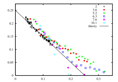
Figure 2: Stationary inclination angle in simple shear flow as function of the rescaled excess area for different viscosity contrasts. The symbols are experimental data from Kantsler and Steinberg Kantsler and Steinberg (2006). The lines represent the linear small deformation theory (40).

Eq. (39) implies that if $\Delta>4h^{2}$, i.e. if the viscosity contrast is higher than a critical value

$${\lambda}_{c}=-\frac{9}{23}+\frac{120}{23}\sqrt{\frac{2\pi}{15\Delta}}$$ (41)

no stationary tank–treading solution exists, as also pointed out by MisbahMisbah (2006); Biben and Misbah (2003), and the vesicle starts to tumble.

IV.2 Tumbling

The second fixed point of Eq. (34) corresponds to periodic vesicle deformation given by oscillating $j=2$ modes around values

$$f_{22}^{\prime}=h({\lambda})\,,\quad f_{22}^{\prime\prime}=0\,\quad f^{\prime}_{21}=0\,,\quad f^{\prime\prime}_{21}=0\,.$$ (42)

If $f_{20}(0)\neq 0$, the $f_{20}(t)$ is also oscillating. All modes with $j\neq 2$ decay to zero and are not oscillating.

The time–periodic vesicle deformation depends strongly on the viscosity contrast as illustrated in Figure 3. Figure 3 (a) shows that close to the critical viscosity contrast the period of oscillations is long and the amplitude of oscillations of the $f_{20}$ mode, which corresponds to out-of-the-flow-plane deformation, is significant. Experimentally the vesicle appears to be trembling or “breathing” Kantsler and Steinberg (2006); Mader et al. (2006). The “breathing” motion has been discussed in parts by Misbah Misbah (2006) although the role of the $f_{20}$ mode has not been recognized.

The mode oscillation frequency increases with viscosity contrast, as seen in Figure 3 (b). At high viscosity contrast it approaches twice the rate of rotation of the external flow, $\dot{\gamma}$. This can be seen from Eq. (34) where in the limit ${\lambda}\gg 1$ only the rotation terms survive. Since the $f_{20}$ mode is not rotationally stabilized, its oscillation amplitude becomes negligible at high viscosity contrast; correspondingly the out-of-the-flow-plane deformation is suppressed. The periodic vesicle deformation then corresponds to rigid body rotation, $f^{\prime}_{22}(t)\sim\cos(t)\,,\quad f^{\prime\prime}_{22}(t)\sim\sin(t)$.

Figure 3: Time dependence of the $f_{2m}$ modes in the (a) breathing (${\lambda}\gtrsim{\lambda}_{c}$) and (b) tumbling (${\lambda}\gg{\lambda}_{c}$) regimes; solid, dashed and dotted lines represent the $f_{22}^{\prime\prime},\,f_{22}^{\prime}$ and $f_{20}$ modes, respectively. The excess area is $\Delta=0.2$. The viscosity contrasts are (a) ${\lambda}=10$,(b) ${\lambda}=100$. The initial conditions are $f^{\prime}_{22}(0)=f^{\prime\prime}_{22}(0)=\sqrt{0.1\Delta}$; $f_{20}(0)$ is determined by the area constraint.

In order to compare theory and experiment we derive expressions for some experimentally measurable parameters. Experimentally only the deformation in the flow plane is observable. The vesicle contour represents an ellipse. Combining (22) and (38) we obtain for the lengths of the major and minor axes

$$r_{max,min}(t)=\textstyle{1-f_{20}(t)\sqrt{\frac{5}{\pi}}\pm\left(\Delta-2f_{20}^{2}(t)\right)^{\frac{1}{2}}\sqrt{\frac{15}{2\pi}}}\,,$$ (43)

where we have neglected the contributions from the $f_{2\pm 1}$ modes for the sake of simplicity. We see that the major and minor axes follow the oscillations of the $f_{20}$ mode: the larger the $f_{20}$ oscillation amplitude, the larger the amplitude in the $r_{max}$ and $r_{min}$ fluctuations. In the experiments of Kantsler and SteinbergKantsler and Steinberg (2006), the excess area $\bar{\Delta}$ corresponding to a prolate ellipsoidal shape with major and minor axes as seen in the flow plane was reported. Using the relation between the deformation in the flow plane and the excess area $(r_{max}-r_{min})/(r_{max}+r_{min})=(15\bar{\Delta}/32\pi)^{\frac{1}{2}}$, reported first by SeifertSeifert (1999a), we obtain

$$\bar{\Delta}(t)=\frac{\Delta-2f^{2}_{20}(t)}{\left[1-f_{20}(t)\sqrt{\frac{5}{16\pi}}\right]^{2}}\,.$$ (44)

Unlike the true excess area $\Delta$, which is constant, $\bar{\Delta}$ is time–dependent due to the fluctuations in the $f_{20}$ mode, i.e. the out-of-the-flow-plane transfer of area.

The angle evolution is described by

$$\dot{\phi}_{0}=-\frac{1}{2}+\frac{h({\lambda})}{(\Delta-2f_{20}^{2}(t))^{\frac{1}{2}}}\cos(2\phi_{0}(t))\,,$$ (45)

from which we infer that the tumbling period, defined as the time needed for a material point to return to its initial position, is given by

$$T_{tumble}=4\pi\left[1-\frac{4h({\lambda})^{2}}{\Delta}\right]^{-{\frac{1}{2}}}\,.$$ (46)

As already discussed, when the viscosity contrast is high the oscillations of the $f_{20}$ mode are suppressed and $f_{20}(t)\approx f_{20}(0)$. In this case Eq. (45) becomes equivalent to the Keller–Skalak equation $\dot{\phi}_{0}=A+B\cos(2\phi_{0})$, where the constants $A$ and $B$ are identified with $-1/2$ and $h({\lambda})/\sqrt{\Delta-2f_{20}^{2}(0)}$, respectively.

We compared the time–dependent vesicle behavior with the experiments of Mader et al.Mader et al. (2006). A good agreement was obtained for the angle evolution, for example of their vesicle number 6 using reduced volume 0.988 instead of the reported 0.996. The difference is reasonable given the uncertainty with which the reduced volume is determined experimentally: it is computed assuming axial symmetry about the vesicle’s longest axis, which might not be always the case because of the presence of a non-zero $f_{20}$ mode. Note, however, that in the tank–treading regime, since the excess area is stored only in the $f_{2\pm 2}$ modes the vesicle is a prolate ellipsoid and the computation of the reduced volume is quite accurate. We also attempted to reproduce theoretically the experimental curves in Figure 4 of Kantsler and SteinbergKantsler and Steinberg (2006). The predicted tumbling frequency from Eq. (46) using viscosity contrast and excess area close to the reported values was almost twice those of the experimental data. One possible explanation is that our small–deformation theory fails for the large values of excess area in this experiment ($\Delta\approx 1$).

IV.3 Rheology

A suspension of vesicles can be described as a continuum with effective properties at length scales large compared to the size of the constituent particles. In dilute suspensions particles are far from each other and they do not feel each others presence. Thus, the effective stress is just a sum of the stress contributions of the individual particles and the bulk stress of a dilute suspension is linear with the particle volume fraction $\varphi$ Kim and Karrila (1991); Pozrikidis (1992)

$$\bm{\Sigma}=2{\bf E}^{s}+\varphi{\bf T}\,,$$ (47)

where ${\bf E}^{s}$ is the symmetric part of the velocity gradient tensor (4) and ${\bf T}$ is the stress associated with the vesicle disturbance velocity field. Rheological properties of interest are the particle contribution to the shear viscosity, $T_{xy}$, and the normal stress differences, $N_{1}=T_{xx}-T_{yy}$ and $N_{2}=T_{yy}-T_{zz}$. Vesicle stress is directly related to the amplitudes of the velocity field $j=2$ (63) Bławzdziewicz et al. (2000) corresponding to the stresslet (the symmetric force dipole). Using the relations (61) we obtain for the vesicle contribution to the effective shear viscosity

$$T_{xy}=\textstyle{\frac{5}{2}\frac{23{\lambda}-39}{23{\lambda}+9}+\chi^{-1}3{\mathrm{i}}\sqrt{\frac{30}{\pi}}\frac{E(2,\sigma_{0})\left(f_{22}-f_{2-2}\right)}{23{\lambda}+9}\,.}$$ (48)

where the shape deformation modes $f_{2\pm 2}$ are given by (81). For a given excess area and viscosity contrast the effective viscosity in the tank–treading regime is

$$T_{xy}=\frac{5}{2}-\Delta\frac{(23{\lambda}+9)}{16\pi}\,,$$ (49)

which is obtained by inserting the expression for the modes amplitude (81) in Eq. (48) and taking into account (83). In the limit of a spherical particle, $\Delta=0$, and since a sphere with fixed area and volume in shear flow undergoes only a rigid body rotation, the Einstein’s result for a suspension of rigid spheres is recovered. The effective viscosity decreases with the increase of the excess area because the deformable vesicles elongate and thus offer less resistance to the flow. An increasing viscosity contrast also leads to a decrease in the effective viscosity because vesicles align better with the flow (the inclination angle (40) decreases with viscosity contrast).

Unlike a suspension of rigid spheres, a suspension of deformable vesicles exhibits normal stresses. In the tank–treading regime below the critical viscosity contrast, the magnitudes of the first normal stress difference is

$$N_{1}=\frac{\Delta(23{\lambda}+9)}{8\pi}\left[-1+\frac{1920\pi}{\Delta(23{\lambda}+9)^{2}}\right]^{\frac{1}{2}}\,,$$ (50)

and the second normal difference is $N_{2}=-{\frac{1}{2}}N_{1}$.

IV.4 Vesicle migration in the presence of a wall

A spherical particle in simple shear flow produces a symmetric disturbance velocity field and therefore the particle does not drift relative to a bounding wall Leal (1980). Particle deformation breaks the symmetry and may lead to cross–stream migration.

The leading order term in the far field of the disturbance velocity due to a force–free and torque–free particle is the stresslet, the symmetric and traceless force dipole. The boundary conditions at the wall can be satisfied by placing the stresslet hydrodynamic image on the opposite sideKim and Karrila (1991). Thus, a particle far away from the wall moves with a velocity due to its corresponding image stresslet; in particular, the vesicle drift velocity normal to a rigid wall is proportional to the stresslet component in the direction of the plane unit normal, i.e. $T_{yy}$. Smart and Leighton Smart and Leighton (1990) report that

$$U_{\mathrm{lift}}=-\frac{3}{16d^{2}}T_{yy}\,,$$ (51)

where $d$ denotes the distance from the particle center to the wall. Taking into account that the normal stress is $T_{yy}=-(N_{1}-N_{2})/3$ and using the normal stresses expressions (50) we obtain for the lift velocity

$$U_{\mathrm{lift}}=\frac{c({\lambda},\Delta)}{d^{2}}\,,$$ (52)

where

$$c({\lambda},\Delta)=\textstyle\frac{3}{32}N_{1}\,.$$ (53)

Similar type expressions have been reported in analytical studies Olla (1997); Seifert (1999b), although the dependence on the excess area has not been presented explicitly. Eq. (53) shows that the more deformable the vesicle, i.e. the larger the excess area, the larger the migration velocity. Interestingly, at very small excess area we obtain from (50) that $N_{1}\sim~{}\Delta^{\frac{1}{2}}$, and vesicle migration is independent of the viscosity contrast. The values of the prefactor (53) are of the same order of magnitude as reported in studies considering a tank-treading ellipsoid Olla (1997) or numerical simulations of a vesicle with no viscosity contrast Sukumaran and Seifert (2001).

V Summary and outlook

This study considers the behavior of a vesicle formed by a fluid membrane in a general shear flow. The analysis takes into account the membrane incompressibility and bending resistance as well as the viscosity contrast between the interior and exterior fluids. Analytical results for a nearly spherical vesicle are obtained. Expressions for the shape evolution equation, stress and velocity fields and the effective membrane tension, which is needed to enforce the area constraint, were derived using a formalism based on spherical harmonics. The main theoretical result of this study is contained in the shape evolution equation Eq. (32) and the expression for the effective tension Eq. (89). The latter serves to eliminate the tension in favor of the excess area, which is the physically relevant parameter. In contrast to drops and capsules, the shape evolution of the area–constrained vesicle is non–linear.

The derived shape evolution equation describes vesicle dynamics in general linear flow. In the particular case of simple shear flow, only the shape modes with the same spherical harmonic order as the external flow, $j=2$, are perturbed; all other modes decay on a time scale set by the bending rigidity. Consequently, the shape evolution equations simplify to Eq. (34) and yield expressions for quantities that can be measured experimentally such as the inclination angle with respect to the flow direction, the lengths of the major and minor axes of the vesicle contour in the flow plane, etc. In the stationary tank–treading state, we show that in a simple shear flow the leading order deformation and stresses are independent of the membrane bending rigidity. Our theory is in quantitative agreement with experimental data for the vesicle deformation in the tank–treading and in the tumbling regimes. Non–Newtonian rheology with normal stresses is predicted for a suspension of vesicles. We also considered the vesicle dynamics in wall–bounded shear flow and presented a simple derivation of the leading order correction, in the distance to the wall, to the rate of vesicle migration away from the wall.

Several problems remain open. We discussed the main features of the time–dependent vesicle dynamics in linear flows, but this problem remains to be systematically explored. Although the quantitative agreement between predicted and experimentally observedMader et al. (2006) behavior of tumbling vesicles with small excess area is encouragingly good, for vesicles with large excess area Kantsler and Steinberg (2006) the agreement is poor, which might be due to the limitations of the leading order theory. Our analysis will be extended to consider higher–order perturbations, and hence elucidate the feedback from the flow on vesicle dynamics.

The developed theory applies only to a nearly spherical vesicle. Larger deformations from sphericity can be explored by numerical simulations. A body of work exists on capsule dynamics, mostly considering elastic membranes with no bending resistance Pozrikidis (1995); Eggleton and Popel (1998); Lac et al. (2004). To our knowledge there are only a couple of numerical studies that include bending resistance Kwak S (2001); Pozrikidis (2001). Area incompressible fluid membranes with bending resistance such as the lipid bilayer membranes, have been studied only to a limited extent Kraus et al. (1996); Beaucourt et al. (2004); Noguchi and Gompper (2005) and some results are conflicting. For example, Noguchi and GompperNoguchi and Gompper (2005) report stationary tank-treading discocyte shape, while Kraus et al.Kraus et al. (1996) find only prolate ones. More efficient and accurate simulations are needed in order to perform a systematic study on flow induced shape transitions. In order to explore numerically the dynamics of highly non–spherical vesicle shapes we are developing Boundary Integral Method simulations, which combine an algorithm for adaptive restructuring of the computational grid that allows resolution of high curvature regionsCristini et al. (2001) with the area constraint (16) and interfacial force density (10).

VI Acknowledgments

RSG acknowledges financial support from the Human Frontier Science Project. PV thanks Rumy Dimova’s group for their the hospitality. This work has benefited from many stimulating discussions with Thomas Powers and Jerzy Blawzdziewicz. The authors thank Reinhard Lipowsky and Markus Deserno for their comments on the manuscript, Manouk Abkarian, Vasiliy Kantsler and Victor Steinberg for providing their experimental data, and Miles Page for proofreading the manuscript.

Appendix A Spherical harmonics

For the sake of completeness, we list the definitions of scalar and vector spherical harmonics Jones (1985); Varshalovich et al. (1988). The normalized spherical scalar harmonics are defined as

$$Y_{jm}\left(\Omega\right)=\textstyle\left[\frac{2j+1}{4\pi}\frac{(j-m)!}{(j+m)!}\right](-1)^{m}P_{j}^{m}(\cos\theta)e^{{\rm i}m\varphi},$$ (54)

where ${\bf\hat{r}}={\bf r}/r$, $(r,\theta,\varphi)$ are the spherical coordinates, and $P_{j}^{m}(\cos\theta)$ are the Legendre polynomials. The vector spherical harmonics are defined as

$${\bf y}_{jm0}=\left[j\left(j+1\right)\right]^{-{\frac{1}{2}}}r\nabla_{\Omega}Y_{jm}\,,$$ (55a)

$${\bf y}_{jm1}=-{\mathrm{i}}{\bf\hat{r}}\times{\bf y}_{jm0}\,,$$ (55b)

$${\bf y}_{jm2}={\bf\hat{r}}Y_{jm}\,,$$ (55c)

where $\nabla_{\Omega}$ denotes the angular part of the gradient operator. ${\bf y}_{jm0}$ and ${\bf y}_{jm1}$ are tangential, while ${\bf y}_{jm2}$ is normal to a sphere.

Appendix B Fundamental set of velocity fields

Following the definitions given in Blawzdziewicz et al.Bławzdziewicz et al. (2000), we list the expressions for the functions ${{\bf u}}^{\pm}_{jmq}\left(r,\Omega\right)$

$$\begin{array}[]{ll}{\bf u}^{-}_{jm0}&={\textstyle\frac{1}{2}}r^{-j}\left(2-j+jr^{-2}\right){\bf y}_{jm0}\\ &+{\textstyle\frac{1}{2}}r^{-j}\left[j\left(j+1\right)\right]^{1/2}\left(1-r^{-2}\right){\bf y}_{jm2}\,,\end{array}$$ (56a)

$${\bf u}^{-}_{jm1}=r^{-j-1}{\bf y}_{jm1}\,,$$ (56b)

$$\begin{array}[]{ll}{\bf u}^{-}_{jm2}&={\textstyle\frac{1}{2}}r^{-j}\left(2-j\right)\left(\frac{j}{1+j}\right)^{1/2}\left(1-r^{-2}\right){\bf y}_{jm0}\\ &+{\textstyle\frac{1}{2}}r^{-j}\left(j+(2-j)r^{-2}\right){\bf y}_{jm2}\,.\end{array}$$ (56c)

$$\begin{array}[]{ll}{\bf u}^{+}_{jm0}&={\textstyle\frac{1}{2}}r^{j-1}\left(-(j+1)+(j+3)r^{2}\right){\bf y}_{jm0}\\ &-{\textstyle\frac{1}{2}}r^{j-1}\left[j\left(j+1\right)\right]^{1/2}\left(1-r^{2}\right){\bf y}_{jm2}\,,\end{array}$$ (57a)

$${\bf u}^{+}_{jm1}=r^{j}{\bf y}_{jm1}\,,$$ (57b)

$$\begin{array}[]{ll}{\bf u}^{+}_{jm2}&={\textstyle\frac{1}{2}}r^{j-1}\left(3+j\right)\left(\frac{j+1}{j}\right)^{1/2}\left(1-r^{2}\right){\bf y}_{jm0}\\ &+{\textstyle\frac{1}{2}}r^{j-1}\left(j+3-(j+1)r^{2}\right){\bf y}_{jm2}\,.\end{array}$$ (57c)

On a sphere $r=1$ these velocity fields reduce to

$${\bf u}^{\pm}_{jmq}={\bf y}_{jmq}\,.$$ (58)

Hence, ${\bf u}^{\pm}_{jm0}$ and ${\bf u}^{\pm}_{jm1}$ are tangential, and ${\bf u}^{\pm}_{jm2}$ is normal to a sphere. In general, a vector velocity field which is tangential to a surface with normal ${\bf n}$ has an irrotational component Bławzdziewicz et al. (1999)

$${\bf n}\cdot\left(\bm{\nabla}_{s}\times{\bf v}^{irr}\right)=0\,,$$ (59)

and solenoidal component

$$\bm{\nabla}_{s}\cdot{\bf v}^{sol}=0\,.$$ (60)

On a sphere, the irrotational component is identified with the $q=0$ vector spherical harmonic, and the solenoidal corresponds to the $q=1$ vector spherical harmonic.

Appendix C Effective stress of a dilute dispersion

The disturbance velocity field due a particle can be represented as a superposition of velocity fields generated by a collection of force multipoles, by analogy to electrostatics Cichocki et al. (1988); Kim and Karrila (1991).

The strength of the stresslet, which is the symmetric and traceless force dipole moment, gives the particle contribution to the effective stress of a dilute dispersion

$$T_{xy}=-\frac{{\mathrm{i}}}{8}\sqrt{\frac{6}{5\pi}}\left(\hat{c}_{220}-\hat{c}_{2-20}\right)\,,$$ (61a)

$$N_{1}=-\frac{1}{4}\sqrt{\frac{6}{5\pi}}\left(\hat{c}_{220}+\hat{c}_{2-20}\right)\,,$$ (61b)

$$N_{2}=-{\frac{1}{2}}N_{1}+\frac{3}{4}\sqrt{\frac{1}{5\pi}}\hat{c}_{200}\,.$$ (61c)

The stresslet field is related to the amplitude of the $j=2$ velocity field; the relations between $\hat{c}$ and $c$ are given by

$$\begin{array}[]{ll}\hat{c}_{jm0}=&\frac{(2j+1)(2j-1)\left[j(j+1)\right]^{1/2}}{j+1}c_{jm0}\\ &+\frac{j(2j+1)(2j-1)}{j+1}c_{jm2}\,.\end{array}$$ (62)

The complete expressions can be found in Blawzdziewicz et al. Bławzdziewicz et al. (2000).

Appendix D Velocity fields and hydrodynamics stresses

Velocity fields are described using basis sets of fundamental solutions of the Stokes equations Cichocki et al. (1988), ${\bf u}^{\pm}_{jmq}$, defined in Appendix B:

$$\begin{split}{\bf v}^{{\mathrm{out}}}\left({\bf r}\right)=&\sum_{jmq}c^{\infty}_{jmq}\left[{\bf u}^{+}_{jmq}\left({\bf r}\right)-{\bf u}^{-}_{jmq}\left({\bf r}\right)\right]\\ &+\sum_{jmq}c_{jmq}{\bf u}^{-}_{jmq}\left({\bf r}\right)\,,\end{split}$$ (63a)

$${\bf v}^{{\mathrm{in}}}\left({\bf r}\right)=\sum_{jmq}c_{jmq}{\bf u}^{+}_{jmq}\left({\bf r}\right)\,.$$ (63b)

The hydrodynamic tractions exerted on a surface with a normal vector ${\bf n}$ are ${\bf n}\cdot{\bf T}$

$$\bm{\tau}\equiv{\bf n}\cdot{\bf T}=\tau_{jmq}{\bf y}_{jmq}$$ (64)

In the particular case of a sphere characterized with a normal vector $\hat{\bf r}$, the viscous tractions are linearly related to the velocity field

$$\tau^{\mathrm{out}}_{jmq}=\sum_{q^{\prime}}^{2}c^{\infty}_{jmq^{\prime}}\left(\Theta_{q^{\prime}q}^{+}-\Theta_{q^{\prime}q}^{-}\right)+\sum_{q^{\prime}}^{2}c_{jmq^{\prime}}\Theta_{q^{\prime}q}^{-}\,$$ (65a)

$$\tau^{\mathrm{in}}_{jmq}=\sum_{q^{\prime}}^{2}c_{jmq^{\prime}}\Theta_{q^{\prime}q}^{+}\,$$ (65b)

where $\Theta_{q^{\prime}q}^{\pm}$ are obtained from the velocity fields (56)–(57) Bławzdziewicz et al. (2000),

$$\Theta^{+}_{qq^{\prime}}\left(j\right)=\left(\begin{array}[]{ccc}2j+1&0&-3\left(\frac{j+1}{j}\right)^{\frac{1}{2}}\\ 0&j-1&0\\ -3\left(\frac{j+1}{j}\right)^{\frac{1}{2}}&0&2j+1+\frac{3}{j}\\ \end{array}\right)$$ (66)

$$\Theta^{-}_{qq^{\prime}}\left(j\right)=\left(\begin{array}[]{ccc}-2j-1&0&3\left(\frac{j}{j+1}\right)^{\frac{1}{2}}\\ 0&-j-2&0\\ 3\left(\frac{j}{j+1}\right)^{\frac{1}{2}}&0&-2j-1-\frac{3}{j+1}\\ \end{array}\right)$$ (67)

In the derivation of the above expressions we have used that

$${\bf\hat{r}}\cdot(\bm{\nabla}{\bf v}+(\bm{\nabla}{\bf v})^{T})=r\frac{d}{dr}\left(\frac{{\bf v}}{r}\right)+\frac{1}{r}\bm{\nabla}\left({\bf v}\cdot{\bf r}\right)\,.$$ (68)

Appendix E Leading order perturbation solution

For small deviations from sphericity Vlahovska et al. (2005), the $O({\varepsilon})$ expansions for the normal vector and the mean curvature are

$${\bf n}\left(\Omega\right)={\bf\hat{r}}-f_{jm}\left[j\left(j+1\right)\right]^{\frac{1}{2}}{\bf y}_{jm0}\,\,,$$ (69)

$$H\left(\Omega\right)=\textstyle{1+\frac{1}{2}\left(j+2\right)\left(j-1\right)f_{jm}Y_{jm}\,.}$$ (70)

At order $O({\varepsilon})$, in the bending stresses (10) the terms $H^{3}$ and $HK$ cancel and only $\nabla_{s}^{2}H$ remains

$$\nabla_{s}^{2}H=-\frac{1}{2}j\left(j+1\right)\left(j-1\right)\left(j+2\right)f_{jm}Y_{jm}\,.$$ (71)

Combining Eqs. (69) and (70) in the Laplace term of the membrane stresses (10) yields

$$\sigma H=\textstyle\left({\frac{1}{2}}\sigma_{0}\left(j-1\right)\left(j+2\right)f_{jm}+\sigma_{jm}\right)Y_{jm}\,.$$ (72)

In the above equation the isotropic part has been omitted because it has no importance to flow dynamics; $\sigma_{jm}f_{jm}$ is neglected as well as it is a higher order term. On a sphere $\nabla_{s}\sigma$ becomes simply $\sqrt{j(j+1)}\sigma_{jm}{\bf y}_{jm0}$ according to Eq. (55a).

All modes that contribute to the excess area are affected by the flow. Therefore, we will present results for any $j$. In this way, the theory can be applied to fluctuating vesicles and other types of flow, e.g. quadratic (Poiseuille) flow.

The incompressibility condition (16) implies that the amplitudes of the velocity disturbance field (63) are related

$$c_{jm2}=\frac{1}{2}\sqrt{j(j+1)}c_{jm0}\,.$$ (73)

At leading order the stress balance reads

$$\hat{\bf r}\cdot{\bf T}^{\mathrm{out}}-({\lambda}-1)\hat{\bf r}\cdot{\bf T}^{\mathrm{in}}={\bf t}^{\mathrm{mem}}\,.$$ (74)

It gives a relation for the tractions (64), which is linear in $j$ and $m$

$$\bm{\tau}^{\mathrm{out}}_{jmq}-({\lambda}-1)\bm{\tau}_{jmq}^{\mathrm{in}}={\bf t}^{{\mathrm{mem}}}_{jmq}\,.$$ (75)

The tangential interfacial stress has an “irrotational” component

$${\bf t}^{\mathrm{mem}}_{jm0}=-\chi^{-1}\sqrt{j(j+1)}\sigma_{jm}\,.$$ (76)

The normal component of the membrane stress is

$${\bf t}^{\mathrm{mem}}_{jm2}=\chi^{-1}\left(2\sigma_{jm}+E(j,\sigma_{0})f_{jm}\right)\,.$$ (77)

The tangential balance (76) determines the tension distribution in terms of the shape parameters

$$\begin{array}[]{ll}\sigma_{jm}&=-\chi c^{\infty}_{jm0}\frac{2\left(1+2j\right)}{\sqrt{j(j+1)}}+\chi c^{\infty}_{jm2}\frac{3(2j+1)}{j(j+1)}\\ &+\chi c_{jm0}\frac{\left(3+{\lambda}\left(j-1\right)\right)}{2\sqrt{j(j+1)}}\,.\end{array}$$ (78)

Finally, the normal stress balance (77) yields $c_{jm0}$.

Expanding around sphere, for the linear flow (3) Eq. (7) yields

$$\frac{\partial f_{jm}}{\partial t}=c_{jm2}+\omega\frac{{\mathrm{i}}m}{2}f_{jm}\quad{\mbox{at}}\,\,r=1\,.$$ (79)

The first term represents the motion of the interface due to the normal component of the velocity and the second term describes the rotation of the deformed shape.

Substituting $c_{jm2}$ in Eq. (79) yields the evolution equation (32) with the following coefficients

$$\begin{array}[]{ll}C({\lambda},j,m)=&d({\lambda},j)^{-1}\left[c^{\infty}_{jm0}\sqrt{j(j+1)}\left(2j+1\right)\right.\\ &\left.+c^{\infty}_{jm2}\left(4j^{3}+6j^{2}-4j-3\right)\right]\end{array}$$ (80a)

and

$$\Gamma\left({\lambda},\sigma_{0},j\right)=-E(j,\sigma_{0})\frac{j(j+1)}{d({\lambda},j)}$$ (80b)

where

$$d({\lambda},j)={9{\lambda}^{-1}+\left(-5+3j^{2}+2j^{3}\right)}$$ (80c)

and

$$E(j,\sigma)=\left(j+2\right)\left(j-1\right)\left(j(j+1)+\sigma\right)\,.$$ (80d)

For a simple shear flow (33), solving Eq.(32) for the stationary amplitudes in the tank-treading regime gives

$$f_{2\pm 2}=\mp\frac{{\mathrm{i}}\chi 10\sqrt{\frac{2\pi}{15}}}{E(2,\sigma_{0})\mp{\mathrm{i}}\chi\frac{(9+23{\lambda})}{6}}$$ (81)

and for the inclination angle

$$\phi_{0}=\frac{1}{2}\arctan\left[\frac{6E(2,\sigma_{0})}{\chi\left(9+23{\lambda}\right)}\right]\,.$$ (82)

These expressions agree with Seifert’s results for a vesicle with no viscosity contrast (${\lambda}=2)$ Seifert (1999a). At long times, the excess area is stored in the $f_{2\pm 2}$ modes only. Substituting the tension (89) in (80d) leads to

$$E(2,\sigma_{0})=\chi\frac{(23{\lambda}+9)}{6}\sqrt{-1+\frac{1920\pi}{(23{\lambda}+9)^{2}\Delta}}.\,$$ (83)

Thus the dependence of the mode amplitudes on the capillary number in Eq.(81) cancels. Expanding Eq. (82) for small values of the excess area $\Delta$ we obtain (40).

The surface solenoidal velocity field ${\bf u}^{\pm}_{jm1}$ satisfies identically the incompressibility condition (16). The stress boundary condition

$$\tau^{\mathrm{out}}_{jm1}-\left({\lambda}-1\right)\tau^{in}_{jm1}=0$$ (84)

corresponds to a spherical viscous drop with no surface tension, i.e. the ${\bf u}^{\pm}_{jm1}$ flow field is unaffected by the interfacial stresses. Consequently, for the $j=1$ component of the shear flow, which corresponds to rigid body rotation, we have that $c_{1m1}=c_{1m1}^{\infty}$, i.e. at leading order the particle rotates with the flow.

For the sake of completeness we mention the relation between our notation and the one used by SeifertSeifert (1999a)

$$\begin{split}c_{jm2}=&X_{jm}\,,\\ c_{jm0}=&\left(Y_{jm}+2X_{jm}\right)\left[j(j+1)\right]^{-{\frac{1}{2}}}\,.\end{split}$$ (85)

Appendix F The isotropic tension

The area constraint (28) serves to determine the isotropic part of the tension $\sigma_{0}$. We can split Eq. (80b) into

$$\Gamma({\lambda},\sigma_{0},j)=\alpha({\lambda},j)+\sigma_{0}\beta({\lambda},j)\,,$$ (86)

where

$$\alpha({\lambda},j)=-2a(j)\frac{[j(j+1)]^{2}}{d({\lambda},j)}\,,$$ (87)

and

$$\beta({\lambda},j)=-2a(j)\frac{j(j+1)}{d({\lambda},j)}\,.$$ (88)

The modes have to satisfy the area constraint $\dot{\Delta}=0$. Multiplying the evolution equations (32) by $a(j)f^{*}_{jm}$ , summing up and solving for the tension leads to

$$\sigma_{0}=-\frac{\sum_{jm}a(j)\left[C({\lambda},j,m)f^{*}_{jm}+\chi^{-1}\alpha({\lambda},j)f_{jm}f^{*}_{jm}\right]}{\chi^{-1}\sum_{jm}a(j)\beta({\lambda},j)f_{jm}f^{*}_{jm}}\,.$$ (89)

The complicated dependence of the tension on the shape modes makes the evolution equations Eq. (32) nonlinear.

References

- Rallison (1984) J. M. Rallison, Ann. Rev. Fluid Mech. 16, 45 (1984).
- Stone (1994) H. A. Stone, Ann. Rev. Fluid Mech. 26, 65 (1994).
- Barthes-Biesel (1991) D. Barthes-Biesel, Physica A 172, 103 (1991).
- Canham (1970) P. Canham, J. Theor. Biol. 26, 61 (1970).
- Powers (2005) T. R. Powers, in Handbook of Materials Modeling, edited by S. Yip (Springer, 2005), pp. 2631–2643.
- Seifert (1997) U. Seifert, Advances in physics 46, 13 (1997).
- de Haas et al. (1997) K. H. de Haas, C. Blom, D. van den Ende, M. H. G. Duits, and J. Mellema, Phys. Rev. E 56, 7132 (1997).
- Kantsler and Steinberg (2005) V. Kantsler and V. Steinberg, Phys. Rev. Lett. 95, 258101 (2005).
- Kantsler and Steinberg (2006) V. Kantsler and V. Steinberg, Phys. Rev. Lett. 96, 036001 (2006).
- Mader et al. (2006) M.-A. Mader, V. Vitkova, M. Abkarian, A. Viallat, and T. Podgorski, Eur. Phys. J. E 19, 389 (2006).
- Kraus et al. (1996) M. Kraus, W. Wintz, U. Seifert, and R. Lipowsky, Phys.Rev.Lett. 77, 3685 (1996).
- Beaucourt et al. (2004) J. Beaucourt, F. Rioual, T. Seon, T. Biben, and C. Misbah, Phys. Rev. E 69, 011906 (2004).
- Noguchi and Gompper (2004) H. Noguchi and G. Gompper, Phys. Rev. Lett. 93, 258102 (2004).
- Seifert (1999a) U. Seifert, Eur. Phys. J. B 8, 405 (1999a).
- Olla (2000) P. Olla, Physica A 278, 87 (2000).
- Misbah (2006) C. Misbah, Phys. Rev. Lett. 96, 028104 (2006).
- Keller and Skalak (1982) S. R. Keller and R. Skalak, J. Fluid Mech. 120, 27 (1982).
- Sutera and Skalak (1993) S. P. Sutera and R. Skalak, Annu. Rev. Fluid Mech. 25, 1 (1993).
- Popel and Johnson (2005) A. S. Popel and P. C. Johnson, Annu. Rev. Fluid Mech. 37, 43 (2005).
- Orsello et al. (2001) C. E. Orsello, D. A. Lauffenburger, and D. A. Hammer, Trends in Biotechnology 19, 310 (2001).
- Lorz et al. (2000) B. Lorz, R. Simson, J. Nardi, and E. Sakmann, Europhys. Lett. 51, 468 (2000).
- Abkarian et al. (2002) M. Abkarian, C. Lartigue, and A. Viallat, Phys. Rev. Lett. 88, 068103 (2002).
- Abkarian and Viallat (2005) M. Abkarian and A. Viallat, Biophys. J. 89, 1055 (2005).
- Cantat and Misbah (1999) I. Cantat and C. Misbah, Phys. Rev. Lett. 83, 235 (1999).
- Sukumaran and Seifert (2001) S. Sukumaran and U. Seifert, Phys. Rev. E 64, 011916 (2001).
- Seifert (1999b) U. Seifert, Phys. Rev. Lett. 83, 876 (1999b).
- Leal (1992) L. G. Leal, Laminar Flow and Convective Transport Processes (Butterworth-Heinemann, Boston, 1992).
- Seifert (1995) U. Seifert, Z. Phys. B 97, 299 (1995).
- Vlahovska et al. (2005) P. Vlahovska, J. Bławzdziewicz, and M. Loewenberg, Phys. Fluids 17, Art. No.103103 (2005).
- Vlahovska (2003) P. Vlahovska, Ph.D. thesis, Yale University (2003), pdf file available by email: petia@aya.yale.edu.
- Barthès-Biesel and Acrivos (1973) D. Barthès-Biesel and A. Acrivos, J. Fluid Mech. 61, 1 (1973).
- Barthes-Biesel (1980) D. Barthes-Biesel, J. Fluid Mech. 100, 831 (1980).
- Biben and Misbah (2003) T. Biben and C. Misbah, Phys. Rev. E 67, 031908 (2003).
- Kim and Karrila (1991) S. Kim and S. J. Karrila, Microhydrodynamics: Principles and Selected Applications (Butterworth-Heinemann, London, 1991).
- Pozrikidis (1992) C. Pozrikidis, Boundary Integral and Singularity Methods for Linearized Viscous Flow (Cambridge University Press, 1992).
- Bławzdziewicz et al. (2000) J. Bławzdziewicz, P. Vlahovska, and M. Loewenberg, Physica A 276, 50 (2000).
- Leal (1980) L. G. Leal, Ann. Rev. Fluid Mech 12, 435 (1980).
- Smart and Leighton (1990) J. R. Smart and D. T. Leighton, Phys. Fluids A 3, 21 (1990).
- Olla (1997) P. Olla, J.Phys. II France 7, 1533 (1997).
- Pozrikidis (1995) P. Pozrikidis, J. Fluid Mech. 297, 123 (1995).
- Eggleton and Popel (1998) C. D. Eggleton and A. S. Popel, Phys. Fluids 10, 1834 (1998).
- Lac et al. (2004) E. Lac, D. Barthes-Biesel, N. Pelekasis, and J. Tsamopolous, J. Fluid Mech. 516, 303 (2004).
- Kwak S (2001) P. C. Kwak S, Phys. Fluids 13, 1234 (2001).
- Pozrikidis (2001) C. Pozrikidis, J. Fluid Mech. 440, 269 (2001).
- Noguchi and Gompper (2005) H. Noguchi and G. Gompper, Phys. Rev. E 72, 011901 (2005).
- Cristini et al. (2001) V. Cristini, J. Bławzdziewicz, and M. Loewenberg, J. Comput. Phys. 168, 445 (2001).
- Jones (1985) M. N. Jones, Spherical Harmonics and Tensors for Classical Field Theory (Wiley, New York, 1985).
- Varshalovich et al. (1988) D. A. Varshalovich, A. N. Moskalev, and V. K. Kheronskii, Quantum Theory of Angular Momentum (World Scientfic, Singapore, 1988).
- Bławzdziewicz et al. (1999) J. Bławzdziewicz, E. Wajnryb, and M. Loewenberg, J. Fluid Mech. 395, 29 (1999).
- Cichocki et al. (1988) B. Cichocki, B. U. Felderhof, and R. Schmitz, PhysicoChem. Hyd. 10, 383 (1988).