Geo-neutrinos: A systematic approach to uncertainties and correlations

Abstract

Geo-neutrinos emitted by heat-producing elements (U, Th and K) represent a unique probe of the Earth interior. The characterization of their fluxes is subject, however, to rather large and highly correlated uncertainties. The geochemical covariance of the U, Th and K abundances in various Earth reservoirs induces positive correlations among the associated geo-neutrino fluxes, and between these and the radiogenic heat. Mass-balance constraints in the Bulk Silicate Earth (BSE) tend instead to anti-correlate the radiogenic element abundances in complementary reservoirs. Experimental geo-neutrino observables may be further (anti)correlated by instrumental effects. In this context, we propose a systematic approach to covariance matrices, based on the fact that all the relevant geo-neutrino observables and constraints can be expressed as linear functions of the U, Th and K abundances in the Earth’s reservoirs (with relatively well-known coefficients). We briefly discuss here the construction of a tentative “geo-neutrino source model” (GNSM) for the U, Th, and K abundances in the main Earth reservoirs, based on selected geophysical and geochemical data and models (when available), on plausible hypotheses (when possible), and admittedly on arbitrary assumptions (when unavoidable). We use then the GNSM to make predictions about several experiments (“forward approach”), and to show how future data can constrain a posteriori the error matrix of the model itself (“backward approach”). The method may provide a useful statistical framework for evaluating the impact and the global consistency of prospective geo-neutrino measurements and Earth models.

1 Introduction

Electron antineutrinos emitted in the decay chains of the heat-producing elements (HPE) U, Th, and K in terrestrial rocks — the so-called geo-neutrinos — represent a truly unique probe of the Earth interior; see [1] for a recent review and [2] for earlier discussions and references. The first indications for a (U+Th) geo-neutrino signal at $>2\sigma$ confidence level in the KamLAND experiment by [3] have boosted the interest in this field, and have started to bridge the two communities of particle physicists and Earth scientists — as exemplarily testified by this Workshop (Neutrino Geophysics, Honolulu, Hawaii, 2005).

The hope is that future measurement of geo-neutrino fluxes can put statistically significant constraints to the global abundances of HPE’s and to their associated heat production rates, which are currently subject to highly debated Earth model assumptions [4; 5]. This goal, despite being experimentally very challenging, is extremely important and deserves dedicated (possibly joint) studies from both scientific communities.

One methodological difficulty is represented by the different “feeling” for uncertainties by particle physicists vs Earth scientists. First important attempts to systematize (U, Th, K) abundance uncertainties in a format convenient for geo-neutrino analyses have been performed in [6] and particularly in [7; 8; 9], where errors have been basically assessed from the spread in published estimates (consistently with mass balance constraints).

We propose to make a further step, by systematically taking into account the ubiquitous error covariances, i.e., the fact that several quantities happen to vary in the same direction (positive correlations) or in opposite directions (negative correlations) in the geo-neutrino context. For instance, in a given Earth reservoir (say, the mantle), the U, Th and K abundances are typically positively correlated. However, they may be anticorrelated in two complementary reservoirs constrained by mass balance arguments, such as the mantle and the crust in Bulk Silicate Earth (BSE) models. Experimental geo-neutrino observables may be further (anti)correlated by instrumental effects.

An extensive discussion of our approach to these problems is beyond the scope of this contribution and will be presented elsewhere [10]. Here we briefly report about some selected issues and results, according to the following scheme. In Sec. 2 we discuss the general aspects and the statistical tools related to covariance analyses, with emphasis on geo-neutrino observables. In Sec. 3 we construct a tentative model for the source distribution of (U, Th, K) in global Earth reservoirs (Geo Neutrino Source Model, GNSM). In Sec. 4 we discuss some issues related to the characterization of local sources around geo-neutrino detector sites. In Sec. 5 and 6 we show examples of “forward” error estimates (i.e., propagation of GNSM errors to predicted geo-neutrino rates) and shortly discuss “backward” error updates (i.e., GNSM error reduction through prospective geo-neutrino data). We draw our conclusions in Sec. 7.

2 Covariance and correlations: General aspects

In this Section we discuss some general aspects of covariance analyses in geochemistry and in neutrino physics, and then present the basic tools relevant for geo-neutrino physics. We remind that, for any two quantities $P$ and $Q$, estimated as

$$P = \overline{P}\pm\sigma_{P}\ ,$$ (1)

$$Q = \overline{Q}\pm\sigma_{Q}\ ,$$ (2)

the correlation index $\rho_{PQ}\in[-1,+1]$ between the 1-$\sigma$ errors of $P$ and $Q$ parameterizes the degree of “covariation” of the two quantities: $\rho>0$ ($<0$) if they change in the same (opposite) direction, while $\rho=0$ if they change independently; see, e.g. [11]. The covariance (or squared error) matrix of $P$ and $Q$ contains $\sigma^{2}_{P}$ and $\sigma^{2}_{Q}$ as diagonal elements, and $\rho_{PQ}\sigma_{P}\sigma_{Q}$ as off-diagonal ones. For more than two variables with errors $\sigma_{i}$ and correlations $\sigma_{ij}$, the covariance matrix is $\sigma^{2}_{ij}=\rho_{ij}\sigma_{i}\sigma_{j}$ (symmetric, with $\rho_{ii}=1$ on the diagonal).

2.1 Covariance analyses in geochemistry

In 1998, the Geochemical Earth Reference Model (GERM) initiative was officially launched [12], in order to provide a “consensus model” for the elemental abundances, together with their errors and correlations, in all relevant Earth reservoirs. Although a lot of work has been done in this direction, e.g., through rich compilations of data and estimates (www.earthref.org), the correlation matrices have not yet been estimated — not even for subsets of elements such as (U, Th, K). To our knowledge, only a few regional studies discuss HPE covariances. These difficulties can be in part overcome by using the (more frequently reported) elemental ratio information. For instance, if the ratio of two abundances $P$ and $Q$ is reported together with its error $\sigma_{P/Q}$, the correlation between $P$ and $Q$ can be inferred through the following statistical relation, valid at first order in error propagation:

$$\left(\frac{\sigma_{P/Q}}{P/Q}\right)^{2}=\Big{(}\frac{\sigma_{P}}{P}\Big{)}^{2}+\Big{(}\frac{\sigma_{Q}}{Q}\Big{)}^{2}-2\rho_{PQ}\Big{(}\frac{\sigma_{P}}{P}\Big{)}\Big{(}\frac{\sigma_{Q}}{Q}\Big{)}\ .$$ (3)

Although the “ratio” and “correlation” information appear to be interchangeable through the above formula, from a methodological viewpoint it is better to use the latter rather than the first, since the ratio of two Gaussian variables is a Cauchy distribution with formally infinite variance [11] — a rather tricky object in statistical manipulations.

2.2 Covariance analyses in neutrino physics

Neutrino physics has undergone a revolution in recent years, after the discovery of neutrino flavor oscillations. Phenomenological fits to neutrino oscillation data have become increasingly refined, and now routinely include covariance analyses (see, e.g., [13]). For our purposes, a relevant example is also given by the Standard Solar Model [14], which provides, among other things, errors and correlations for solar neutrino sources. We shall try to apply a similar “format” to a geo-neutrino source model in Sec. 3.

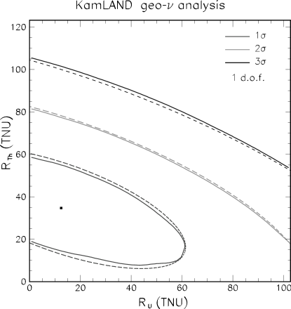
Figure 1: Best-fit U and Th event rates and error contours (solid lines) from our analysis of KamLAND geo-neutrino data [10]. The contours are very close to two-dimensional Gaussian confidence levels (dashed ellipses). Units: 1 TNU = 1 event/year/$10^{32}$ target protons.

Correlations arise not only at the level of neutrino sources, but also at the detection level, as a consequence of instrumental effects. For instance, the KamLAND experiment is currently more sensitive to the sum (U+Th) of geo-neutrino fluxes rather than to the separate U and Th components. As a consequence, the measured U and Th geo-neutrino event rates are anticorrelated: if one rate increases the other one tends to decrease, in order to keep the total rate constant (within errors).

Figure 1 shows explicitly the anticorrelation between the U and Th experimental rates through their 1, 2, and 3-$\sigma$ contours (solid lines) taken from our KamLAND data analysis [10]. The contours in Fig. 1 are well approximated by a bivariate gaussian (dashed lines) with parameters:

$$R_{\mathrm{U}}=12.5\pm 48.9\mathrm{\ TNU},\ R_{\mathrm{Th}}=34.7\pm 28.5\mathrm{\ TNU},\ \rho=-0.645\ .$$ (4)

We have also verified that our KamLAND data analysis reproduces the confidence level contours in the alternative plane spanned by $R_{\mathrm{U}}+R_{\mathrm{Th}}$ and $(R_{\mathrm{U}}-R_{\mathrm{Th}})/(R_{\mathrm{U}}+R_{\mathrm{TH}})$ [3] (not shown); however, as explained in the previous subsection, we prefer to avoid any “ratio” and to use just $(R_{\mathrm{U}},\,R_{\mathrm{Th}})$ and their correlation.

2.3 General tools for geo-neutrinos

In the context of geo-neutrinos, statistical analyses are greatly simplified by the fact that all relevant observables are linear combinations of the HPE abundances $a^{\mathrm{S}}_{i}$ in different reservoirs (S = U, Th, K; $i=$ reservoir index), with coefficient determined by known physics and by the geometry of the Earth mass distribution.

Table 1: Universal (reservoir-independent and detector site-independent) coefficients for the calculation of the total heat ($H$) of the Earth, and of the total $\overline{\nu}_{e}$ flux ($\Phi_{D}$) and event rates from inverse beta decay ($R_{D}$) at any detector site $D$. Conversion factors: 1 TNU = 1 event/year/$10^{32}$ target protons; 1 year = $3.15576\times 10^{7}$ s. Natural abundances of isotopes are assumed.

	$h_{\mathrm{S}}$	$\phi_{\mathrm{S}}$	$r_{\mathrm{S}}$
S	($\mu$W/kg)	($10^{12}$ $\overline{\nu}_{e}$/cm2/s)	($10^{8}$ TNU)
U	98.0	123	15.2
Th	26.3	26.1	1.06
K	$34.9\times 10^{-4}$	$45.4\times 10^{-3}$	0

In particular we consider: ($i$) the total radiogenic heat $H$ of the Earth (decay energy absorbed per unit of time); ($ii$) the geo-neutrino flux $\Phi_{D}$ at a given detector site $D$ (number of $\overline{\nu}_{e}$ per unit of area and time); and ($iii$) the corresponding event rate $R_{D}$ at a given detector site $D$ (number of events from $\overline{\nu}_{e}+p\to n+e^{+}$, per unit of time and of target protons). Such quantities can be written as:

$$H_{R} = \sum_{\mathrm{S}}h_{\mathrm{S}}\sum_{i}M_{i}\,a_{i}^{\mathrm{S}}\ ,$$ (5)

$$\Phi_{D} = \langle P_{ee}\rangle\sum_{\mathrm{S}}\phi_{\mathrm{S}}\sum_{i}f_{i}^{D}\,a_{i}^{\mathrm{S}}\ ,$$ (6)

$$R_{D} = \langle P_{ee}\rangle\sum_{\mathrm{S}}r_{\mathrm{S}}\sum_{i}f_{i}^{D}\,a_{i}^{\mathrm{S}}\ ,$$ (7)

where the universal coefficients $h_{\mathrm{S}}$, $\phi_{\mathrm{S}}$, and $r_{\mathrm{S}}$, according to our calculations [10], are given in Table 2.3. In the above equations, $M_{i}$ is the mass of the $i$-th reservoir, while $\langle P_{ee}\rangle\simeq 0.57$ is the average survival oscillation probability of geo-$\overline{\nu}_{e}$. The geometrical coefficients $f_{i}^{\mathrm{D}}$ represent the mass-weighted average of the inverse square distance of the detector site $D$ from the $i$-th reservoir, necessary to account for the flux decrease with distance; their numerical values will be reported elsewhere [10].

The Earth mass distribution necessary to compute the $M_{i}$’s and $f_{i}^{\mathrm{D}}$’s is taken from the Preliminary Earth Reference Model (PREM) [15], properly matched with a crustal model defined over a grid of $2^{\circ}\times 2^{\circ}$ tiles [16]. The Earth is assumed to be partitioned into the following homogeneous reservoirs: core, lower mantle, upper mantle, continental crust (in three layers—upper, middle, lower) and oceanic crust (lumped into one layer). The distinction (if any) between lower and upper mantle is strongly debated and will be commented later. For a set of possible geo-neutrino detector sites (Kamioka, Gran Sasso, Sudbury, Hawaii, Pyhäsalmi, Baksan), we consider “local” reservoirs, defined as the nine (three-by-three) tiles of the $2^{\circ}\times 2^{\circ}$ model which surround each detector site—except for Kamioka, where 13 tiles are considered, corresponding to the “Japanese arc and forearc” as defined in the crustal model [16]. Due to the inverse-squared-distance decrease of the neutrino flux, it turns out that local and global reservoirs can provide comparable contributions to the geo-neutrino event rates, at least for detectors sitting on the continental crust.

The main task is then to build a model for the abundances $a_{i}^{\mathrm{S}}$, embedding covariances. In other words, by switching to a single-index vector notation for simplicity,

$$\left\{a^{\mathrm{S}}_{i}\right\}^{\mathrm{S=U,Th,K}}_{i=1,\dots,N}\to\mathbf{a}=\left\{a_{i}\right\}_{i=1,\dots,3N}\$$ (8)

(where $N$ is the number of reservoirs), an Earth model should provide, for any entry in the HPE abundance vector $\mathbf{a}$, both a central value $\overline{a}_{i}$ and a standard deviation $\pm\sigma_{i}$,

$$a_{i}=\overline{a}_{i}\pm\sigma_{i}$$ (9)

together with the error correlation matrix $\rho$. The components of the covariance matrix ${\mbox{\boldmath$\sigma$}}^{2}$ are then

$$[{\mbox{\boldmath$\sigma$}}^{2}]_{ij}=\rho_{ij}\sigma_{i}\sigma_{j}\ .$$ (10)

Given any two quantities $P$ and $Q$ [as in Eqs. (5)–(7)] defined as linear combinations of the $a_{i}$’s (with $T=$ transpose),

$$P = \sum_{i}p_{i}a_{i}={\mbox{\boldmath$p$}}^{T}{\mbox{\boldmath$a$}}\ ,$$ (11)

$$Q = \sum_{i}q_{i}a_{i}={\mbox{\boldmath$q$}}^{T}{\mbox{\boldmath$a$}}\ ,$$ (12)

it turns out that their 1-$\sigma$ errors $\sigma_{P}$ and $\sigma_{Q}$ are simply given by

$$\sigma^{2}_{P} = \sum_{ij}p_{i}p_{j}\rho_{ij}\sigma_{i}\sigma_{j}={\mbox{\boldmath$p$}}^{T}{\mbox{\boldmath$\sigma$}}^{2}{\mbox{\boldmath$p$}}\ ,$$ (13)

$$\sigma^{2}_{Q} = \sum_{ij}q_{i}q_{j}\rho_{ij}\sigma_{i}\sigma_{j}={\mbox{\boldmath$q$}}^{T}{\mbox{\boldmath$\sigma$}}^{2}{\mbox{\boldmath$q$}}\ ,$$ (14)

with $(P,Q)$ correlation given by

$$\rho_{PQ}=\frac{\sum_{ij}p_{i}q_{j}\rho_{ij}\sigma_{i}\sigma_{j}}{\sigma_{P}\sigma_{Q}}=\frac{{\mbox{\boldmath$p$}}^{T}{\mbox{\boldmath$\sigma$}}^{2}{\mbox{\boldmath$q$}}}{\sigma_{P}\sigma_{Q}}\ .$$ (15)

The above equations will be used below to compute correlations among experimental event rates, or between an experimental rate and the radiogenic heat.

3 Towards a Geo-Neutrino Source Model (GNSM)

In this Section we briefly discuss our methodology to provide entries for Eqs. (9,10), i.e., a Geo-Neutrino Source Model for HPE abundances in the Earth. We remind that, concerning the entries for Eq. (9) (errors only, no correlations), our approach overlaps in part with earlier relevant work performed in [1; 7; 9].

3.1 The Bulk Silicate Earth

Bulk Silicate Earth (BSE) models [4] provide global constraints on elemental abundances (especially in the primitive mantle), under a set of hypotheses. In particular, BSE models include the plausible assumption that elements which have both high condensation temperature (“refractory”) and that are preferentially embedded in rocks rather in iron (“lithophile”) should be found in the primitive mantle (i.e., in the undifferentiated mantle+crust reservoir) in the same ratio as in the parent, pristine meteoritic material. Among the three main HPE’s (U, Th, K), the first two are also refractory lithophile elements (RLE), so the Th/U global ratio should be the same in BSE and in the (supposedly) parent and most primitive meteoritic material (carbonaceous chondrites CI). Our summary [10] of the recent and detailed works on absolute [17; 18] and relative [19; 20] U and Th abundances in CI meteorites (with $1\sigma$ errors) is:

$$a^{\mathrm{Th}}_{\mathrm{CI}} = 30.4(1\pm 0.10)\times 10^{-9}\ ,$$ (16)

$$a^{\mathrm{U}}_{\mathrm{CI}} = 8.10(1\pm 0.10)\times 10^{-9}\ ,$$ (17)

$$\left(a^{\mathrm{Th}}_{\mathrm{CI}}/a^{\mathrm{U}}_{\mathrm{CI}}\right) = 3.75(1\pm 0.05)\ ,$$ (18)

which implies a (Th,U) error correlation $\rho_{\mathrm{CI}}=0.875$ through Eq. (15).

The BSE/CI abundance ratio is expected to be the same for all RLE’s, if indeed they did not volatilize during the Earth formation history. The benchmark is usually provided by a major RLE element such as Al, which, being much more abundant than the trace elements Th and U, can be more robustly constrained, both by mass-balance arguments and by direct sampling. Our summary [10] for the BSE/CI abundance ratio of Al from three detailed BSE models [17; 21; 22] is

$$\left(a^{\mathrm{Al}}_{\mathrm{BSE}}/a^{\mathrm{Al}}_{\mathrm{CI}}\right)=2.7(1\pm 0.10)\ .$$ (19)

The previous arguments and estimates imply that

$$a^{\mathrm{Th}}_{\mathrm{BSE}}=a^{\mathrm{Th}}_{\mathrm{CI}}\cdot\left(a^{\mathrm{Al}}_{\mathrm{BSE}}/a^{\mathrm{Al}}_{\mathrm{CI}}\right) = 82.1(1\pm 0.14)\times 10^{-9}\ ,$$ (20)

$$a^{\mathrm{U}}_{\mathrm{BSE}}=a^{\mathrm{Th}}_{\mathrm{CI}}\cdot\left(a^{\mathrm{Al}}_{\mathrm{BSE}}/a^{\mathrm{Al}}_{\mathrm{CI}}\right) = 21.9(1\pm 0.14)\times 10^{-9}\ ,$$ (21)

with (Th,U) error correlation $\rho_{\mathrm{BSE}}=0.936$.

The K element, being (moderately) volatile, needs a separate discussion. In [23] it was argued that U is a good “global” proxy for K, since: (1) the K/U abundance ratio was found to be nearly constant in 22 samples of Mid-Ocean Ridge Basalt (MORB) from the Atlantic and Pacific ocean floor (thought to be representative of the whole mantle); (2) the MORB K/U ratio was found to be (accidentally) similar to the K/U ratio estimate in the crust from an older model [24]. The MORB K/U ratio ($1.27\times 10^{4}$) was then boldly generalized to the whole Earth, with small estimated errors (1.6%) [23]. However, it should be noticed there are no geochemical arguments to presume that disparate elements such as U and K should have the same partition coefficients between melt (= crust) and residual mineral (= depleted mantle); indeed, analogous alleged coincidences have later been disproved [25]. Therefore, we think that the “canonical K/U=12,700” ratio, so often quoted in the geochemical literature, should be critically revisited in future studies. Provisionally, from a survey of recent literature about the abundances of K and U (and of another possible K-proxy element, La [17]) in MORB databases, continental crust samples and estimates, and BSE models, we are inclined to [10]: (1) increase significantly — although subjectively — the K/U uncertainty; and (2) slightly lower the central value (as compared with [23]). More precisely, we take

$$\left(a^{\mathrm{K}}_{\mathrm{BSE}}/a^{\mathrm{U}}_{\mathrm{BSE}}\right)=1.2\times 10^{4}(1\pm 0.15)\ ,$$ (22)

which, by proper error propagation, gives the absolute K abundance as

$$a^{\mathrm{K}}_{\mathrm{BSE}}=263\times 10^{-6}(1\pm 0.21)\ ,$$ (23)

with (K,Th) and (K,U) correlations equal to 0.648 and 0.701, respectively. Table 2 presents a summary of the BSE (U, Th, K) abundances, errors and correlation matrix, together with similar information about the main BSE sub-reservoirs (as discussed below).

Needless to say, all the above BSE estimates may be significantly altered, if possible indications for nonzero HPE abundances in the Earth core [26] are corroborated by further studies. For the sake of simplicity, we do not consider such possibility in this work.

Table 2: Geo-Neutrino Source Model (GNSM): Abundances, errors and correlations of radiogenic elements (U, Th, K) in global reservoirs.

Geo-Neutrino Source Model (GNSM)				Correlation matrix
for global reservoirs				BSE			CC			OC			UM			LM
Reser.	Elem.	Abundance	$\pm 1\sigma$	U	Th	K	U	Th	K	U	Th	K	U	Th	K	U	Th	K
	U	$21.9\times 10^{-9}$	$\pm 14\%$	1	$+.936$	$+.701$	0	0	0	0	0	0	0	0	0	$+.908$	$+.893$	$+.690$
BSE	Th	$82.1\times 10^{-9}$	$\pm 14\%$		1	$+.648$	0	0	0	0	0	0	0	0	0	$+.850$	$+.954$	$+.638$
	K	$26.3\times 10^{-5}$	$\pm 21\%$			1	0	0	0	0	0	0	0	0	0	$+.636$	$+.618$	$+.985$
	U	$1.46\times 10^{-6}$	$\pm 17\%$				1	$+.906$	$+.906$	0	0	0	0	0	0	$-.409$	$-.263$	$-.146$
CC	Th	$6.29\times 10^{-6}$	$\pm 10\%$					1	$+.595$	0	0	0	0	0	0	$-.371$	$-.291$	$-.096$
	K	$1.62\times 10^{-2}$	$\pm 10\%$						1	0	0	0	0	0	0	$-.371$	$-.173$	$-.161$
	U	$1.00\times 10^{-7}$	$\pm 30\%$							1	$+.906$	$+.868$	0	0	0	$-.012$	$-.007$	$-.007$
OC	Th	$2.20\times 10^{-7}$	$\pm 30\%$								1	$+.764$	0	0	0	$-.011$	$-.007$	$-.006$
	K	$1.25\times 10^{-3}$	$\pm 28\%$									1	0	0	0	$-.010$	$-.006$	$-.008$
	U	$3.95\times 10^{-9}$	$\pm 30\%$										1	$+.906$	$+.868$	$-.093$	$-.065$	$-.058$
UM	Th	$10.8\times 10^{-9}$	$\pm 30\%$											1	$+.764$	$-.084$	$-.071$	$-.051$
	K	$5.02\times 10^{-5}$	$\pm 28\%$												1	$-.081$	$-.054$	$-.066$
	U	$17.3\times 10^{-9}$	$\pm 27\%$													1	$+.924$	$+.692$
LM	Th	$60.4\times 10^{-9}$	$\pm 27\%$														1	$+.640$
	K	$21.7\times 10^{-5}$	$\pm 36\%$															1

3.2 The Continental Crust (CC)

Average elemental abundances in the continental crust (CC), and their vertical distribution in the three main identifiable layers (upper, middle, lower crust = UC, MC, LC), have been presented in a recent comprehensive review [27], together with a wealth of data and with a critical survey of earlier literature on the subject. In particular, it is stressed in [27] that some previous CC models are not consistent with known crustal heat production constraints [28]. This fact shows that: (1) the spread of published values for elemental abundances is not necessarily indicative of the real uncertainties, since some estimates can be invalidated by new and independent data; (2) heat production estimates in the CC provide a relevant constraint (linear in the U, Th, K crustal abundances) which might help, together with geo-neutrino measurements, to reduce the HPE abundance estimates in reference models. The latter point will be further elaborated elsewhere [10].

We basically adopt the results in [27] for the UC, MC, LC abundances of (U, Th, K) and their uncertainties, with the following differences: (1) since no error estimates are given for the LC, we conservatively (but arbitrarily) assume fractional $1\sigma$ errors of $40\%$ in this layer; (2) our reference crustal model [16] and the one in [27] provide mass ratios among layers (UC:MC:LC) respectively equal to 0.359:0.330:0.311 and 0.317:0.296:0.387. This difference is somewhat disappointing, since it induces weighted-average HPE abundance shifts in the CC of order $10\%$, which are definitely nonnegligible. “Consensus values” for the mass distribution in the three CC layers (upper, middle, lower) would thus be desirable in the future. Provisionally, we assume that CC elemental abundance errors cannot be smaller than the “mass distribution” induced error (10%). We also assume, from a survey of the relevant literature, a $9\%$ fractional error for each of the K/U, Th/U, and K/Th ratios in the crust — which in turn provide the (U, Th, K) correlations [10]. Given such inputs, the CC abundances (central values, errors, and correlations) turn out to be as shown in Table 2.

3.3 The Upper Mantle (UM)

We assume a homogeneous composition for the upper mantle (defined as the sum of transition zone + low-velocity zone + “lid” in the PREM model [15]). Global and detailed analyses of all the available upper mantle samples and constraints have been performed in two recent papers [29; 30] which, unfortunately, do not really agree in their conclusions, despite being based in part on the same petrological database (www.petdb.org). Concerning HPE’s, we then take as central values the average of [29] and [30], but we attach the most conservative error estimates of [29], which are large enough to cover the spread between [29] and [30]. We assume a K/U ratio error in the upper mantle of the same size as for the BSE ($\pm 15\%$), and a Th/U ratio error of $\pm 13\%$, as suggested from the scatter of points in Fig. 2 of [29]. Given such inputs, the UM abundances turn out to be [10] as shown in Table 2.

3.4 The Oceanic Crust (OC)

The oceanic crust is difficult to sample and, not surprisingly, only a few papers (to our knowledge) deal with its average trace-element composition (see, e.g., [31; 32; 33]). We adopt the “intermediate” central values of [31], which suggest a HPE enrichment of the oceanic crust by a factor 20–25 with respect to the (parent) upper mantle. Since the enrichment is approximately uniform for all three HPE’s, we think it reasonable to assume that the same relative spread of abundances is transferred from the UM (parent mineral) to the OC (melt). Therefore, in the absence of other information, we attach to the (U, Th, K) abundances in the OC the same fractional errors and correlations as for the UM, see Table 2.

3.5 The Lower mantle (LM)

The consistent derivation of LM abundances, errors and correlations is a qualifying result of our work. The abundances in the lower mantle (LM) are obtained by subtraction (LM=BSE-UM-CC-OC), namely, by the mass balance constraint:

$$a^{\mathrm{S}}_{\mathrm{LM}}=(a^{\mathrm{S}}_{\mathrm{BSE}}M_{\mathrm{BSE}}-a^{\mathrm{S}}_{\mathrm{UM}}M_{\mathrm{UM}}-a^{\mathrm{S}}_{\mathrm{CC}}M_{\mathrm{CC}}-a^{\mathrm{S}}_{\mathrm{OC}}M_{\mathrm{OC}})/M_{\mathrm{LM}}\ ,$$ (24)

for S=U, Th, K. Since the three HPE abundances $a^{\mathrm{S}}_{\mathrm{LM}}$ are linear combinations of BSE, UM, CC, and OC abundances, it is possible to apply the formalism of Sec. 2.3 and to obtain their errors and correlations, whose numerical values are listed in Table 2 (last three columns). It turns out that the LM fractional uncertainties are comparable to those of the UM ($\sim 30\%$), and that the LM abundances are strongly correlated with the BSE ones but moderately anticorrelated with the CC ones, due to the subtraction procedure. The LM anticorrelation with the UM and OC is instead very small, since the latter two reservoirs contain relatively small absolute amounts of HPE’s, as compared to the CC and BSE.

Once the LM contents of HPE’s are obtained, the BSE information becomes redundant, and one can proceed with the information contained in the 12 entries for the (CC, OC, UM, LM) abundances, and the corresponding $12\times 12$ correlation matrix, which are reported in Table 2. Notice that, within the quoted uncertainties, the abundances in Table 2 are consistent with those reported in [8].

3.6 What about Mantle Convection?

There is currently a strong debate about the nature and extent of mantle convection, with scenarios ranging from two-layer models (with geochemically decoupled UM and LM) to whole mantle convection (with completely mixed UM and LM), and many intermediate possibilities and variants [4; 34]. Two extreme possibilities are: (1) a geochemically homogeneous mantle (i.e., no difference between UM and LM, $a^{\mathrm{S}}_{\mathrm{LM}}=a^{\mathrm{S}}_{\mathrm{UM}}$); and (1) a strict two-layer model (i.e., a lower mantle conserving primitive mantle abundances, $a^{\mathrm{S}}_{\mathrm{LM}}=a^{\mathrm{S}}_{\mathrm{BSE}}$).

Our estimates in Table 2 are intermediate between such two cases, and thus agree better with models predicting partial mantle mixing. The two extreme cases are anyway recovered by stretching the uncertainties to roughly $\pm 3\sigma$. Fig. 2 shows the 1, 2, and $3\sigma$ error ellipses in the (LM,UM) and (LM,BSE) Uranium abundance planes; within $3\sigma$, both cases $a^{\mathrm{U}}_{\mathrm{LM}}=a^{\mathrm{U}}_{\mathrm{UM}}$ and $a^{\mathrm{U}}_{\mathrm{LM}}=a^{\mathrm{U}}_{\mathrm{BSE}}$ (slanted lines) are allowed. Similar results are obtained for Th and K (not shown). Therefore, our GNSM estimates are sufficiently conservative to cover, within $\pm 3\sigma$, a wide spectrum of mantle mixing scenarios (two-layer convection, partial UM-LM mixing, whole mantle convection).

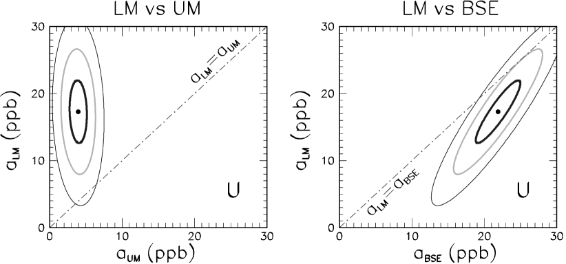
Figure 2: Comparison between LM, UM, and BSE abundances of Uranium, in ppb ($10^{-6}$) units. Our GNSM estimates are shown as 1, 2, and 3$\sigma$ error ellipses. The slanted lines represent the cases of whole mantle convection (in the left panel) and of decoupled LM (in the right panel).

4 Issues related to “local” reservoirs

In our work, local reservoirs have been arbitrarily defined as the nine crustal tiles around each detector (except for Kamioka), see Sec. 2.3. Here we discuss some issues related to this or other choices for the “local” contribution to geo-neutrino fluxes.

4.1 What is a “local” reservoir?

It is necessary to define in some way “local” reservoirs, since the crust (and perhaps the mantle) within a few hundred km from each detectors site may well be different from the average crust defined in the previous section. This fact has already been recognized in [6; 9], where “local” HPE abundances for the Kamioka site have been estimated. The boundaries of the local crust are matter of convention — but any convention is not without consequences, however. In particular, in our approach, we observe that the correlation between “local” reservoirs and “global” ones (LM, UM, OC, CC) is expected to vanish: the uncertainty of the U abundance near the Kamioka mine has probably nothing to do with the errors of the whole CC and OC crust estimates. However, only dedicated studies, which should take into account all locally homogenous geochemical micro-reservoirs and their correlation lengths with farther geo-structures, can provide a physically motivated distinction between local and global reservoirs—a task much beyond the scope of this work. For simplicity, we just assume that all local-to-global abundance correlations are exactly zero.

4.2 Horizontal and vertical (U, Th, K) distribution uncertainties

Assuming that a “local” reservoir is defined in some way, its volumetric distributions of HPE’s can significantly affect the estimated geo-$\nu$ fluxes, due to the inverse square distance dependence. In principle, one would like to have such detailed information around each detector site, both horizontally and vertically. In practice, however, one usually has mainly scattered “surface” samples and only weak constraints about the vertical HPE distribution. Although the HPE abundances are expected to decrease with depth, the decrease may be highly site-dependent and non-monotonic (see [35] as an example for the Japanese crust). In some cases (e.g., Sudbury [36]) the horizontal and vertical distributions of HPE’s are correlated by the fact that the crust is locally “tilted” — a situation which may represent both a complication and an opportunity.

In all cases, significant progress in the characterization of the HPE volumetric distribution in local reservoirs can be obtained only by dedicated geophysical and geochemical studies, which should collect all the (currently sparse and partly unpublished) relevant pieces of data, including representative rock samples, local crustal models, and heat flow measurements. Some interesting work in this direction has been done for the Kamioka site [6; 9], showing that a $O(10\%)$ uncertainty in the local geo-neutrino flux (at $1\sigma$) may perhaps be reachable. We think that $10\%$ should be the “target error” for the characterization of the local geo-neutrino flux at each detector site. Much larger errors would hide information coming from farther reservoirs, and in particular from the mantle.

4.3 Provisional assumptions

In order to make provisional numerical estimates, we make the following assumptions for local HPE abundances in the crust: (1) we assume the same numerical values and errors as for the average upper, middle, and lower crust estimates [27] discussed in Sec. 3.2, except for the Kamioka site where the average upper crust abundances are taken from the thorough geochemical study in [37]; (2) we assume that the correlations between local and global abundances, as well between local crust layers, are zero; (3) we assume a plausible (but arbitrary) hierarchy of correlations between HPE abundances in each layer: $\rho(\mathrm{U,Th})=0.8$, $\rho(\mathrm{U,K})=0.7$, $\rho(\mathrm{K,Th})=0.6$, implying that Th is a good proxy for U and that K is a somewhat worse proxy for both U and Th (as it generally happens in other reservoirs). Further comments about such choices are given elsewhere [10]. As previously remarked, the admittedly arbitrary assumptions characterizing local contributions to geo-$\nu$ fluxes can and should be improved by dedicated inter-disciplinary studies.

5 Forward propagation of uncertainties

We have described in Sec. 2 a possible path towards the definition of a GNSM, i.e., of a set of HPE abundances, errors and correlations in a given partition of the Earth into global and local reservoirs. We now show examples of propagation of such uncertainties, according to Eqs. (11)–(15).

5.1 Errors and correlations at a specific site (Kamioka)

Figure 3 shows our estimated geo-neutrino event rates from U and Th decays at the Kamioka site (including neutrino oscillations with $\langle P_{ee}\rangle=0.57)$, superposed to the same experimental (gaussian) contours as in Fig. 1. The numerical values for the GNSM predictions are:

$$R_{\mathrm{U}}=24.9\pm 2.0\mathrm{\ TNU},\ R_{\mathrm{Th}}=6.7\pm 0.5\mathrm{\ TNU},\ \rho=+0.902\ .$$ (25)

The correlation between the theoretical rates is positive, since Th and U are good proxies of one another in each reservoir. The total (U+Th) rate in Kamioka is also positively correlated with the total (U+Th+K) radiogenic heat $H$ in the Earth. We estimate:

$$R_{\mathrm{U+Th}}=31.6\pm 2.5\mathrm{\ TNU},\ H=21.1\pm 3.0\mathrm{\ TW},\ \rho=+0.858\ .$$ (26)

The strong correlation between $R_{\mathrm{U+Th}}$ and $H$ implies that a precise measurement of the former would yield a robust constraint on the latter. Unfortunately, the experimental errors in Fig. 3 are still much larger than the theoretical (GNSM) ones, implying that, at present, the first KamLAND data do not significantly constrain plausible Earth models and the associated radiogenic heat (see also [38]). Patient accumulation of statistics, significant reduction of background and systematics, and new independent experiments, are required to test and constrain typical Earth model predictions.

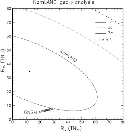
Figure 3: U and Th geo-neutrino event rate predictions from our tentative GNSM at Kamioka (small ellipses with positive correlations), superposed to the same KamLAND experimental constraints as in Fig. 1. In both cases, the 1, 2, and $3\sigma$ contours are shown. Current experimental errors appear to be significantly larger than the “theoretical” GNSM ones.

5.2 Errors and correlations among different sites

Table 3 shows our estimates for the total (U+Th) rates (central values and $\pm 1\sigma$ error) at different possible detector sites, together with their correlation matrix. Correlations are always positive (when one rate increases, any other is typically expected to do the same), but can either be strong (such as between Gran Sasso and Pyhäsalmi, both located in somewhat similar CC settings), or relatively weak (such as between any “continental crustal site” and the peculiar “oceanic site” at Hawaii, which sits on the mantle). Such correlations should be taken into account in the future, when data from two or more detectors will be compared with Earth models.

Table 3: Expected total neutrino event rates (U+Th), together with their errors and correlations, as calculated for different sites within the GNSM, assuming $\langle P_{ee}\rangle=0.57$.

	Rate (U+Th)	Correlation matrix
Site	$\pm 1\sigma$ (TNU)	Kam.	Gra.	Sud.	Haw.	Pyh.	Bak.
Kamioka (Japan)	$31.60\pm 2.46$	1.000	0.722	0.649	0.825	0.630	0.624
Gran Sasso (Italy)	$40.55\pm 2.86$		1.000	0.707	0.641	0.734	0.700
Sudbury (Canada)	$47.86\pm 3.23$			1.000	0.554	0.688	0.652
Hawaii (USA)	$13.39\pm 2.21$				1.000	0.484	0.510
Pyhäsalmi (Finland)	$49.94\pm 3.45$					1.000	0.692
Baksan (Russia)	$50.73\pm 3.41$						1.000

6 Backward update of the GNSM error matrix

As shown in Fig. 3, the first KamLAND data do not yet constrain our tentative GNSM. However, it is tempting to investigate the impact of future, high-statistics and multi-detector geo-neutrino data on the model. In particular, one might try to estimate what are the HPE abundances which best fit both the starting GNSM and a set of prospective, hypothetical experimental data (“backward” update of GNSM errors). It can be shown that the covariance formalism allows to reduce this problem to matrix algebra [10].

Here we give just a relevant example of possible results, in an admittedly optimistic future scenario where all 6 detectors in Table 3 are operative and collect separately U and Th events for a total exposure of 20 kilo-ton year, at exactly the predicted rate, with no background and no systematics. In such scenario, the mantle and BSE uranium abundance errors would be reduced as in Fig. 4, which should be compared with the previous estimates in Fig. 2. It can be seen that, in principle, the depicted scenario might allow to reject at $\gg 3\sigma$ the case $a_{\mathrm{LM}}=a_{\mathrm{UM}}$, i.e., of global mantle convection, which would be a really relevant result in geophysics and geochemistry. Needless to say, more realistic (and less optimistic) simulations of prospective data need to be performed in order to check if similar goals can be experimentally reached. In any case, our approach may provide a useful template for such numerical studies.

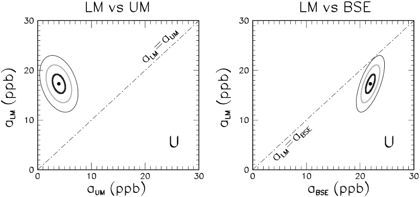
Figure 4: As in Fig. 2, but including constraints from a hypothetical data set from six detectors running for 20 kTy in ideal conditions. See the text for details.

7 Conclusions and prospects for further work

In this contribution to the Hawaii Workshop on Neutrino Geophysics (2005) we have briefly presented a systematic approach to the ubiquitous issue of covariances in geo-neutrino analyses. Correlations among the abundances of (U,Th,K) in each reservoir and among different reservoirs, as well as covariances between any two linear combinations of such abundances (including neutrino fluxes, event rates, heat production rates) have been treated in a statistically consistent way. A tentative Geo Neutrino Source Model (GNSM)—embedding a full error matrix for the (U,Th,K) abundances in relevant local and global reservoirs—has been built, based on published data (when available) and on supplementary assumptions (when needed). The construction of the GNSM highlights some crucial issues that should be solved by dedicated studies, in order to get the most from future geo-neutrino data. Applications of our approach have been given in terms of predictions for future experiments (“forward” propagation of errors) and of GNSM error reduction through prospective data (“backward” update of uncertainties). Inter-disciplinary studies of more refined geochemical and geophysical Earth models, and of future possible observations of geo-neutrino signals, are needed to quantify more realistically both the assumed uncertainties and the future impact of geo-neutrino data in Earth sciences.