Violation of market efficiency in transition economies

Abstract

We analyze the European transition economies and show that time series for most of major indices exhibit (i) power-law correlations in their values, power-law correlations in their magnitudes, and (iii) asymmetric probability distribution. We propose a stochastic model that can generate time series with all the previous features found in the empirical data.

An interesting question in economics is whether markets in transition economies defer in their behavior from developed capital markets. One way to analyze possible differences in behavior is to test the weak form of market efficiency that states that the present price of a stock comprises all of the information about past price values implying that stock prices at any future time cannot be predicted. In contrast to predominant behavior of financial time series of developed markets characterized by no or very short serial correlations Fama65 ; Gra64 ; Sha77 ; hiemstra , it is believed that financial series of emerging markets exhibit different behavior jagric .

For ten transition economies in east and central Europe with statistics reported in Table 1, we analyze time series of index returns $R_{t}=\log S(t+\Delta t)-\log S(t)$, daily recorded.

Table 1 shows that none of the index time series $R_{t}$ exhibits a vanishing skewness defined as a measure of asymmetry — $\langle(x-\mu)^{3}\rangle/\sigma^{3}$ — where $\mu$ and $\sigma$ are the expectation and the standard deviation, respectively. Five of time series show positive skewness, i.e., their probability distributions have more pronounced right tail, while the rest five time series exhibit negative skewness. Fig. 1 shows the probability distribution $P(R_{t})$ of the BUX index with negative skewness and the Gaussian distribution clearly with vanishing skewness.

Next we calculate the kurtosis defined as $\langle(x-\mu)^{4}\rangle/\sigma^{4}$ that is e.g. for a Gaussian distribution equal to 3. Generally, for a probability distribution with more (less) weight in the tails, the kurtosis is greater (smaller) than 3. Table 1 shows that for none of the ten index time series the observed probability distribution is a Gaussian.

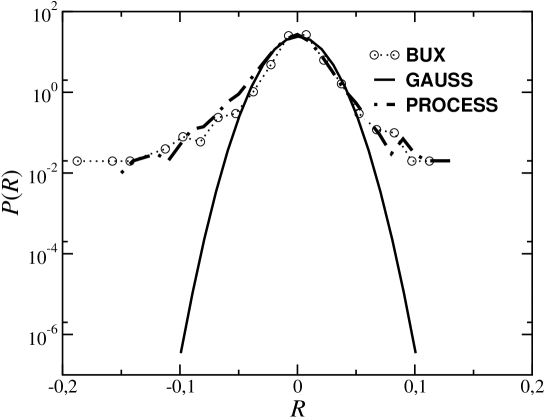
Figure 1: Probability distribution of $R_{t}$ calculated for the BUX index and the Gaussian distribution with the same standard deviation as found for the BUX index. The kurtosis of $P(R_{t})$ for the BUX index is $17$, which is much greater than the kurtosis of the Gaussian probability distribution, which is $3$. We see that $P(R_{t})$ for the BUX index is negatively skewed, in opposite to the Gaussian that is symmetric. Shown is $P(R_{t})$ of the process with $\rho_{1}=0.09$, $\rho_{2}=0.3$, and $\lambda=-0.2$

To analyze correlations in time series, we employ the detrended fluctuation analysis (DFA)  CKP , the wavelet analysis and the Geweke and Porter-Hudak (GPH) method  GPH . The detrended fluctuation function $F(n)$ follows a scaling law $F(n)\propto n^{\alpha}$ if the time series is power-law auto-correlated. A DFA scaling exponent $\alpha>~{}0.5$ corresponds to time series with power-law correlations, and $\alpha=0.5$ corresponds to time series with no auto-correlations. For GPH method, the process is said to exhibit long memory if the GPH parameter $d$ is from the range $(0,0.5)$.

For each of ten indices time series $R_{t}$, Table 1 shows the DFA scaling exponent $\alpha$, Hurst exponent $H$ calculated by wavelet analysis, and the GPH parameter $d$. We show that DFA and wavelet analysis give similar results. Besides SAX and perhaps WIG20 index, the other indices exhibit power-law serial correlations. Similar results are obtained by GPH method where the relation $\alpha=0.5+d$ is expected in presence of power-law correlations.

Next, we calculate the DFA scaling exponents $\alpha_{|R|}$ for the time series of $|R_{t}|$. From Table 2 we see that for each index, the time series $|R_{t}|$ shows power-law auto-correlations, a common behavior on stock markets, where generally $\alpha_{|R|}>\alpha_{R}$.

In order to investigate to which degree the ten time series exhibit linear and nonlinear properties Euro ; Ashk20 , we phase randomize the original time series where the procedure changes (does not change) magnitude auto-correlations for a nonlinear (linear) process PodHosk . During phase-randomization procedure one performs a Fourier transform of the original time series and then randomizes the Fourier phases keeping the Fourier amplitudes unchanged. At the end, one calculates an inverse Fourier transform and obtains the surrogate time series $\tilde{R}_{t}$.

For the BUX index, Fig. 2 shows the DFA functions $F(n)$ of the time series $R_{t}$ and $|R_{t}|$ together with $F(n)$ of the phase-randomized surrogate time series $\tilde{R}_{t}$ and $|\tilde{R}_{t}|$. As expected, the $F(n)$ curves of $R_{t}$ and $\tilde{R}_{t}$ are the same Euro . In contrast, the time series $|\tilde{R}_{t}|$ is uncorrelated $(\alpha_{|\tilde{R}|}=0.5)$, while the time series $|R_{t}|$ is power-law auto-correlated $(\alpha_{|R|}=0.8)$. Similar behavior in scaling of time series we find for all other 10 indices (see Table 1).

Next we propose a stochastic process to model time series $R_{t}$ with power-law correlations in both $R_{t}$ and $|R_{t}|$ together with asymmetric probability distributions $P(R_{t})$  ASYMM

$$R_{i} = \sum_{n=1}^{\infty}{a_{n}(\rho_{1})}[R_{i-n}-\lambda|R_{i-n}|]+\sigma_{i}\eta_{i},$$ (1)

$$\sigma_{i} = \sum_{n=1}^{\infty}{a_{n}(\rho_{2})}\frac{|R_{i-n}|}{\langle|R_{i}|\rangle}.$$ (2)

The weights defined as $a_{n}(\rho)=\rho{\Gamma(n-\rho)}/({\Gamma(1-\rho)\Gamma(1+n)})$ for $n>>1$ scales as $a_{n}(\rho)\propto n^{1-\rho}$, where $\rho_{1/2}~{}\epsilon~{}(0,0.5)$ are scaling parameters. It holds that $\sum_{n=1}^{\infty}a_{n}(\rho)=1$. If asymmetry parameter $\lambda$ is zero, the process is a combination of two fractionally integrated processes in Refs. Granger80 ; Hosk81 and Granger96 . $\Gamma$ is a Gamma function, and $\eta_{i}$ denotes Gaussian white noise with $\langle\eta_{i}\rangle=0$ and $\langle\eta_{i}^{2}\rangle=\sigma_{0}^{2}$, where $\sigma_{0}^{2}$ we set to model the variance of empirical data.

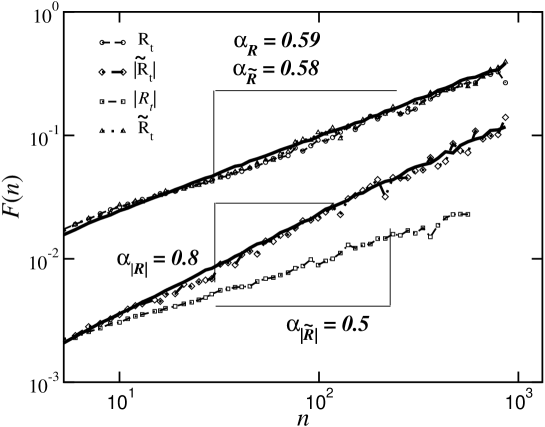
Figure 2: Time series of returns $R_{t}$ of Hungarian BUX index. DFA functions calculated for four time series: $R_{t}$, the one obtained after phase-randomization procedure $\tilde{R}_{t}$, and two magnitudes time series; $|R_{t}|$ and $|\tilde{R}_{t}|$. After phase randomization procedure, the time series $|\tilde{R}_{t}|$ has no auto-correlations. By solid lines we show $R_{t}$ and $|R_{t}|$ of the process with $\lambda=-0.2$, $\rho_{1}=0.09$, and $\rho_{2}=0.3$

In Ref. PodHosk for the case $\lambda=0$, $\rho_{1}=\rho_{2}=\rho$ $(\rho_{1,2}>0.5)$, we derived the following two scaling relations $\alpha_{R}=0.5+\rho$ and $\alpha_{|R|}=0.5+\rho$ between two DFA exponents $\alpha_{R}$ and $\alpha_{|R|}$ and $\rho$. To model empirical time series with different exponents $\alpha_{R}$ and $|\alpha_{R}|$, we allow $\rho_{1}$ and $\rho_{2}$ to be different.

Applied the process to model empirical data, first we calculate DFA exponents $\alpha_{R}$ and $\alpha_{|R|}$ and if $\alpha_{R}<\alpha_{|R|}$, we calculate $\rho_{1}$ and $\rho_{2}$ from scaling relations $\alpha_{R}=0.5+\rho_{1}$ and $\alpha_{|R|}=0.5+\rho_{2}$, respectively. For the Hungarian BUX index, from the DFA exponents $\alpha_{R}=0.59$ and $\alpha_{|R|}=0.8$ (see Table 1) and previous scaling relations, we calculate the parameters $\rho_{1}=0.09$ and $\rho_{2}=0.3$. In Fig. 2 we show the scaling function $F(n)\propto n^{\alpha}$ for both model time series $R_{t}$ and $|R_{t}|$ (solid lines), where we arbitrarily set $\lambda=-0.2$ to account for small skewness in the empirical distribution. After performing phase-randomization procedure, auto-correlations in $|\tilde{R}_{t}|$ vanish, while auto-correlations in $\tilde{R}_{t}$ practically remain the same as in the original time series $R_{t}$, that is the same behavior as we found in empirical data. In Fig.1 we also find that $P(R_{t})$ calculated for the process fits $P(R_{t})$ calculated for the BUX index.

In conclusion, we show that for ten transition economies their market indices analyzed exhibit (i) power-law correlations in index returns, (ii) power-law correlations in the magnitudes, where the probability distributions exhibit (iii) asymmetric behavior. These three properties we model with a stochastic process specified by only three parameters.

country	$Rus$	$Hun$	$Pol$	$Slovak$	$Sloven$	$Czech$	$Lit$	$Lat$	$Est$	$Cro$
index	$RTS$	$BUX$	$WIG20$	$SAX$	$SBI$	$PX50$	$VILSE$	$RICI$	$TALSE$	$CROEMI$
st. dev.	$0.031$	$0.017$	0.022	0.014	0.014	$0.014$	0.007	0.010	0.019	0.014
skewness	$-0.344$	$-0.865$	-0.446	-0.409	0.416	$1.342$	$-1.065$	1.240	2.944	0.731
kurtosis	$7.96$	$17.69$	11.97	9.48	25.34	17.18	26.89	22.46	47.80	12.51
$\alpha_{R_{t}}$	$0.60$	$0.59$	$0.52$	$0.53$	$0.62$	$0.63$	$0.63$	$0.58$	$0.70$	0.58
$\alpha_{|R_{t}|}$	$0.79$	$0.80$	$0.84$	$0.66$	$0.74$	$0.86$	$0.69$	$0.65$	$0.80$	0.70
$\alpha_{\tilde{R}_{t}}$	$0.59$	$0.58$	$0.52$	$0.51$	$0.58$	$0.67$	$0.63$	$0.56$	$0.69$	0.57
$\alpha_{|\tilde{R}_{t}|}$	$0.51$	$0.50$	$0.45$	$0.53$	$0.51$	$0.47$	$0.54$	$0.55$	$0.53$	0.52
data points	$2232$	$3373$	$2530$	$2204$	$2884$	$2567$	$1829$	$2025$	$183$	1522

Table 1: Basic statistics of financial data. Besides skewness and kurtosis, which are the measures for asymmetry and ”fatness” in the tails, also shown is DFA exponents for time series of indices and their magnitudes together with the corresponding values obtained after phase randomization.

country	Rus	Pol	Czech	Hun	Slovak	Sloven	Cro	Lith	Latv	Est
index	RTS	WIG20	PX50	BUX	SAX	SBI	CROEMI	VILSE	RICI	TALSE
$\alpha_{R}$	0.60	0.56	0.63	0.59	0.53	0.62	0.58	0.63	0.58	0.70
$H$	0.65	0.57	0.65	0.63	0.53	0.66	0.62	0.63	0.62	0.65
$d$	0.11	0.02	0.27	0.07	0.01	0.14	0.10	0.10	0.15	0.07

Table 2: Scaling exponents calculated for DFA method, wavelet method and GPH method.

References

- (1) E. F. Fama, J. Business 38, 34 (1965).
- (2) C.W.J. Granger and O. Morgenstern (1963).
- (3) J. L. Sharma and R. E. Kennedy, J. Fin Qua Analysis 12(3), 391 (1977)
- (4) C. Hiemstra and J.D. Jones, J. Emp. Finance 4, 373 (1997).
- (5) T. Jagric, B. Podobnik and M. Kolanovic, East. Econ. 72, (2005).
- (6) C.-K. Peng et al., Phys. Rev. E 49, 1685 (1994).
- (7) J. Geweke and S. Porter-Hudak, J. Time Series Analysis 4. 221 (1983)
- (8) J. Theiler et al., Physica D 58, 77 (1992).
- (9) Y. Ashkenazyet al., Phys. Rev. Lett. 86, 1900 (2001).
- (10) B. Podobnik et al., Phys. Rev. E 72, 026121 (2005).
- (11) B. Podobnik et al., Phys. Rev. E 71, 025104 (2005).
- (12) C. W. J. Granger and R. Joyeux, J. Time Series Analysis 1, 15 (1980).
- (13) J. Hosking, Biometrika 68, 165 (1981).
- (14) C. W. J. Granger and Z. Ding, J. Econometrics 73, 61 (1996).
- (15) John T. Barkoulas, Christopher F. Baum, Economies Letters 53, 253 (1996).