Energy Linearity and Resolution of the ATLAS Electromagnetic Barrel Calorimeter in an Electron Test-Beam

Abstract

A module of the ATLAS electromagnetic barrel liquid argon calorimeter was exposed to the CERN electron test-beam at the H8 beam line upgraded for precision momentum measurement. The available energies of the electron beam ranged from $10$ to $245$ GeV. The electron beam impinged at one point corresponding to a pseudo-rapidity of $\eta=0.687$ and an azimuthal angle of $\phi=0.28$ in the ATLAS coordinate system. A detailed study of several effects biasing the electron energy measurement allowed an energy reconstruction procedure to be developed that ensures a good linearity and a good resolution. Use is made of detailed Monte Carlo simulations based on GEANT4 which describe the longitudinal and transverse shower profiles as well as the energy distributions. For electron energies between $15$ GeV and $180$ GeV the deviation of the measured incident electron energy over the beam energy is within $0.1\%$. The systematic uncertainty of the measurement is about $0.1\%$ at low energies and negligible at high energies. The energy resolution is found to be about $10$% $\cdot\sqrt{E}$ for the sampling term and about $0.2$% for the local constant term.

, , , , , , , , , , , , , , , , , , , , , , , , , , , , , , , , , , , , , , , , , , , , , , , , , , , , , , , , , , , , , , , , , , , , , , , , , , , , , , , , , , , , , , , , ,

Introduction

The Large Hadron Collider (LHC), currently under construction at CERN, will collide protons on protons with a beam energy of $7$ TeV, extending the available centre-of-mass energy by about an order of magnitude over that of existing colliders. Together with its high collision rate, corresponding to an expected integrated luminosity of $10-100~{}{\mathrm{fb}}^{-1}/{\mathrm{year}}$, these energies allow for production of particles with high masses or high transverse momenta or other processes with low production cross-sections. The LHC will search for effects of new interactions at very short distances and for new particles beyond the Standard Model of particle physics (SM). The large particle production rates at LHC are not only a challenge to our theoretical understanding of proton proton collisions at such high energies, but also for the detectors.

An excellent knowledge of the electron or photon energy is needed for precision measurements of, for example couplings within and beyond the SM, or to resolve possible narrow resonances of new particles over a large background. A good energy resolution and a good linearity need to be achieved for energies ranging from a few GeV up to a few TeV.

A prominent example is the possible discovery of the Higgs boson which in the SM provides an explanation how the elementary particles acquire mass. If the Higgs boson mass is below $130$ GeV, the decay $H\rightarrow\gamma\gamma$ is the most promising discovery channel. If the Higgs mass is larger and, in particular if it is at least twice the mass of the $Z^{0}$-boson $2\,M_{Z}\sim 180$ GeV, the Higgs boson can be discovered in the $H\rightarrow Z^{0}Z^{0}\rightarrow e^{+}e^{-}e^{+}e^{-}$ decay channel. Even in this case the energy of one of the electrons can be as low as about $10$ GeV. The possible observation of the Higgs boson requires therefore excellent measurements of electrons and photons from low to high energies.

The absolute energy measurement can be calibrated on reference reactions as $pp\to Z^{0}X\to e^{+}e^{-}X$, exploiting the precise knowledge of the mass of the $Z^{0}$-boson. However, a good energy resolution and a good linearity can only be achieved, if the detector, the physics processes in the detector, and effects of the read-out electronics are well understood. In particular, knowledge of the detector linearity determines how precisely an energy measurement at one particular energy can be transfered to any energy. For instance, to measure the mass of the $W^{\pm}$-boson with a precision of $15$ MeV a linearity of about $10^{-4}$ is required in an energy interval which is given by the difference of the transverse energy spectrum of an electron from the $W^{\pm}$-boson decay and that of the $Z^{0}$-boson [1].

The electromagnetic (EM) barrel liquid argon (LAr) calorimeter is the main detector to measure the electron energy in the central part of the ATLAS detector. It is a sampling calorimeter with accordion shaped lead absorbers and LAr as active medium.

In August $2002$ a production module of the ATLAS LAr EM barrel calorimeter was exposed to an electron beam in the energy range of $10$ to $245$ GeV at the CERN H8 beam line, which was upgraded with a system to precisely measure the beam energy. These data are used to assess the linearity of the electron energy measurement and the energy resolution. A calibration scheme is developed which ensures simultaneously a good linearity and a good resolution.

In the past the linearity of the ATLAS EM calorimeter has been studied with a calorimeter prototype [2]. For electron energies between $20$ - $300$ GeV a linearity within $1$% has been measured.

In section 1 the system to measure the linearity of the beam energy is presented and its accuracy is discussed. Section 2 describes the ATLAS EM barrel calorimeter, the H8 test-beam set-up, the data samples, and the event selection. The Monte Carlo simulation is out-lined in section 3. Section 4 summarises the calibration of the electronic signal, converting the measured current to a visible energy, i.e., the energy deposited in the active medium. Section 5 discusses general effects related to the physics of EM showers that need to be taken into account to precisely reconstruct the electron energy. Section 6 presents the calibration procedure to precisely reconstruct the total electron energy. Comparison of the visible energies and the total reconstructed energy in the data and in the Monte Carlo simulation are shown in section 7. The possible pion contamination in the electron beam is discussed in section 8. The results of the energy measurement together with their systematic uncertainties are presented in section 9.

1 Precise Determination of the Relative Electron Beam Energy

1.1 The H8 Beam-line

The H8 beam line is sketched in Fig. 1. The electron momentum definition is based on the second momentum analysis using two triplets of bending magnets B3 and B4, between collimator C3 acting as a source, and collimator C9 acting as a momentum slit, while the upstream part was set at $180$ GeV. A thin sheet of lead was introduced upstream of C3 to increase the electron yield. The magnets were set in direct current (DC) mode and the induced current was read-out with a Direct Current Current Transformer (DCCT).

To control the induced current in the spectrometer with a single precision DCCT, only the B3 magnets, connected in series, were used. This limited the maximum momentum to $180$ GeV for a current of about $1200$ A. The B4 magnets were degaussed, following a bipolar loop and kept unpowered. The remaining bending power $\int Bdl$ was zero with an uncertainty of $\pm 1.5$ mT $\cdot$ m. Each bending magnet has an effective length of $5.2$ m and a field of $1.42$ T/kA (linear part).

To eliminate any uncertainty coming from the geometry of the spectrometer, the jaw positions of both C3 and C9 were kept fixed during the entire data taking period. A slit of $8$ mm was chosen for C3 as a compromise between the beam intensity and the momentum spread. The slit of C9 was kept at $8$ mm. The induced momentum spread was $\pm 0.15$ % at all energies. With the geometry of the spectrometer fixed (its total deviation is $41$ mrad) the momentum of selected electrons is directly proportional to the bending power $\int Bdl$ of the B3 triplet. A correction of half the energy lost by synchrotron radiation in the spectrometer was applied to particles at the detector, downstream of C9.

The effect of the earth’s field along the beam line was also evaluated. Taking into account the focusing effect of the quadrupoles with the beam transport program TURTLE[20], the net effect found was a shift of $+4$ MeV for negative particles.

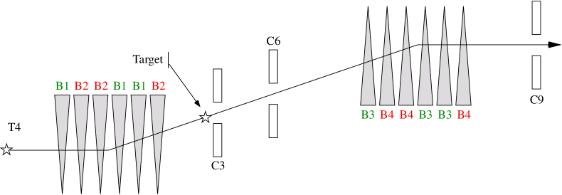
Figure 1: Sketch of the H8 beam line showing the momentum definition elements. The magnets labeled B4 were degaussed during the data taking period.

1.2 Control of the Beam Energy Linearity

Two main sources of uncertainties on the power of the bending magnets had to be controlled:

1. The value of the current in the magnet string:
   The precision supply and the DCCT read-out ensured a relative precision and reproducibility of $1\cdot 10^{-4}$ [3, 4, 5, 6].

2. The calibration and reproducibility of the hysteresis curve:
   At the maximum current of $1200$ A, the integral bending power is about $2$% below the linear extrapolation from low currents (see Fig. 2). This needed to be calibrated and the non-linearity controlled to about one percent.

A reference magnet (MBN25) was calibrated using a precision power supply and the DCCT, and a two wire loop to measure its bending power. The magnetic field at the centre was also measured with a relative precision better than $1\cdot 10^{-5}$ using a set of NMR probes [3, 4] Results are shown in Fig. 2. The measurements can be fitted with a polynomial function. The residuals are smaller than $10^{-4}$.

To transport this calibration to the B3 triplet, calibration curves measured during the time of production of about $100$ MBN magnets were used to compare the reference magnet and the magnets of the B3 triplet. While all magnets had been trimmed during production to be identical within $\pm 2\cdot 10^{-4}$ [7, 8], a small difference (at most $3\cdot 10^{-4}$ at the highest current) between the reference magnet and the B3 triplet had to be corrected.

To ensure reproducibility of the field for a given current, the same unipolar setting loop was always used, both in the bench test and during setting up with the beam. With this procedure, the uncertainty on the bending power is $1$ mT $\cdot$ m at all energies.

In order to have a further cross-check of the actual field in the B3 triplet during electron data taking, one of the magnets of the triplet was instrumented with two sets of Hall probes, to be read-out during each burst. They were positioned at $1.0$ m and $1.5$ m inside the magnet, within a few mm from the vacuum pipe. The Hall probes data include Hall voltages for three orthogonal directions, and the temperature. A correction of about $-3\cdot 10^{-4}/^{o}C$ for the magnetic field as measured with the Hall probes was applied. By running the Hall probes positioned in the reference magnet at the same location as in the B3 magnets, a cross calibration with respect to the current in the DCCT, the magnetic field at centre, and the bending power was obtained.

A critical test of the cross calibration of the two field measurements in B3 is a comparison of the magnetic field at the magnet centre calculated from the DCCT current and from the Hall probe signals. Fig. 3 shows an excellent agreement up to $400$ A and a small systematic inhomogeneity ($0.15$%) at the maximum current. This difference is attributed to a slight difference of the field at the Hall probe location, which is not taken into account by the comparative calibration. A linear interpolation of the differences leaves an average dispersion of $2\cdot 10^{-4}$ which indicates the level of uncertainty on the linearity induced by taking one measurement or the other.

1.3 Results and Uncertainties

For the final comparison of the beam energy with the electron energy reconstructed in the calorimeter, the bending power calculated from the DCCT current was used. For each run the DCCT currents read-out at each burst were averaged. The currents were stable within $0.01$ A.

The resultant beam energy determinations are summarised in Tab. 1. The synchrotron radiation correction includes small additional losses in the correction magnets (B5 and B6) downstream of C9.

Since this work does not aim at a precise absolute calibration, the electron beam energy was arbitrarily normalised at $100$ GeV. The maximum induced uncertainty on the synchrotron radiation loss is $15$ MeV at $180$ GeV. The magnet correction corresponds to the difference between MBN25 and the three magnets of the B3 string.

The largest uncertainty is associated to the remnant field in B3 ($\pm 1$ mT $\cdot$ m randomly on each energy point). The resulting uncertainty on the linearity measurement estimated with a simple Monte Carlo simulation where a perfect linearity is assumed and the beam momenta fluctuate according to their uncertainties is $3\cdot 10^{-4}$. A further systematic uncertainty of $11$  MeV due to the remnant fields in the B4 magnets must be added. This last uncertainty is common to all data points.

Figure 2: a) Calibration measurements of the magnetic field integrated over the beam path as a function of the induced current. The adjusted parameterisation is superimposed as line. b) Deviation from linearity, i.e., measured field values divided by a linear parameterisation obtained from the points below $I<500$ A as a function of the induced current.

Figure 3: Difference between the values of the magnetic field at the magnet centre, predicted by the calibration obtained from the current measurements and the magnetic field measurements with the Hall probe as a function of the current. The error bars represent the root mean square of the distribution.

events	nom. E	current	$\int Bdl$	magnet	syn. rad. corr.	E
	[ GeV ]	[A]	[T $\cdot$ m]	corr.	[ GeV ]	[ GeV ]
$6703$	$10.$	$62.315$	$1.3664$	$0.99975$	$0.0000$	$10.092\pm 0.013$
$2727$	$15.$	$93.133$	$2.0379$	$0.99975$	$0.0000$	$15.041\pm 0.009$
$6463$	$20.$	$124.363$	$2.7184$	$0.99975$	$0.0001$	$20.061\pm 0.010$
$6746$	$25.$	$155.513$	$3.3980$	$0.99975$	$0.0003$	$25.074\pm 0.011$
$8403$	$30.$	$186.689$	$4.0789$	$0.99975$	$0.0006$	$30.098\pm 0.012$
$7842$	$35.$	$217.900$	$4.7607$	$0.99975$	$0.0012$	$35.128\pm 0.013$
$8791$	$40.$	$248.973$	$5.4397$	$0.99975$	$0.0020$	$40.137\pm 0.014$
$8314$	$45.$	$280.075$	$6.1201$	$0.99975$	$0.0032$	$45.148\pm 0.014$
$18366$	$50.$	$311.270$	$6.8005$	$0.99975$	$0.0049$	$50.174\pm 0.017$
$9465$	$60.$	$373.484$	$8.1596$	$0.99975$	$0.0102$	$60.197\pm 0.020$
$9507$	$70.$	$435.705$	$9.5187$	$0.99975$	$0.0189$	$70.216\pm 0.022$
$9829$	$80.$	$497.673$	$10.8715$	$0.99976$	$0.0322$	$80.184\pm 0.025$
$9973$	$90.$	$559.524$	$12.2208$	$0.99976$	$0.0515$	$90.120\pm 0.028$
$22685$	$100.$	$621.128$	$13.5634$	$0.99976$	$0.0781$	$100.000\pm 0.033$
$9585$	$120.$	$744.113$	$16.2383$	$0.99980$	$0.1605$	$119.658\pm 0.037$
$9367$	$150.$	$926.708$	$20.1866$	$0.99995$	$0.3806$	$148.594\pm 0.046$
$4960$	$180.$	$1115.230$	$24.1095$	$1.00011$	$0.7698$	$177.182\pm 0.056$

Table 1: Summary of the used data sets. Number of the selected electron events, nominal beam energy, induced current in the magnetic field, magnet bending power, corrections for magnets and synchrotron radiation and the measured beam energy. The overall beam momentum scale is normalised to $100$ GeV. At $E=245\mbox{\rm~{}GeV}~{}$no precision energy measurement is possible with the used magnet set-up.

2 Test-Beam Set-up and Event Selection

2.1 Test-Beam Set-up

The H8 test-beam set-up is shown in Fig. 4. The EM barrel calorimeter is located in a cryostat filled with liquid argon (LAr). The cryostat consists of an inner and an outer aluminum wall with thicknesses of $4.1$ cm and $3.9$ cm, respectively. The two walls are separated by a vacuum gap. Between the cryostat and the calorimeter module a foam block (ROHACELL) is installed to exclude LAr in front of the calorimeter.

The cryostat is mounted on a table that allows rotation of the calorimeter in the two directions orthogonal to the beam axis. The two directions are chosen to be the $\eta$ and $\phi$ directions with respect to a reference frame with cylindrical coordinates having its origin in the virtual proton-proton interaction point in ATLAS (see Fig. 4). In this coordinate system the $z$-axis is defined along the beam axis. The $\phi$ and $\theta$ angles are the azimuthal and polar angles. The pseudo-rapidity is defined by $\eta=-\log{\tan{\theta/2}}$.

In front of the cryostat four multi-wire proportional chambers (BC1, BC2, BC3, BC4) measured the position of the beam particles. Three scintillator counters (S1,S3,S4) located in between the wire chambers were used as event trigger. The last two (S3 and S4) each with a size of $4$x$4$ cm were used to define the beam acceptance and to reject events with more than one charged track. Since in the test-beam particles hit the calorimeter at random times with respect to the $40$ MHz clock used by the front-end electronics, the time between a trigger and the next clock cycle was measured with a Time Digital Converter (TDC) with a $50$ ps/TDC-count sensitivity.

Behind the calorimeter and after about $13$$X_{0}$ of material (including cryostat and a $5$ cm lead plate) a scintillator was installed to reject pions (pion counter). Another scintillator was installed after an iron block of $5$ interaction lengths to reject muons. For most of the runs both scintillators have been used on-line to reject muons and pions.

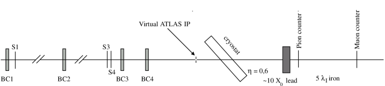
Figure 4: Schematic top view of the test-beam set-up.

2.2 The ATLAS Electromagnetic Barrel Calorimeter

The details of the ATLAS LAr barrel calorimeter are described elsewhere [2, 9]. A module is made out of accordion shaped lead absorbers glued between two $0.2\mbox{\rm~{}mm}~{}$thick stainless steel sheets placed into a cryostat containing LAr. The read-out electrodes are interleaved between two absorbers. At $\eta=0.687$, the lead of the absorbers have a thickness of $1.53\mbox{\rm~{}mm}~{}$ and the gap size is about $2.1\mbox{\rm~{}mm}~{}$on each side of the electrode.

The module is longitudinally segmented into three compartments, each having a different transverse segmentation. At $\eta=0.687$, the front, middle and back compartments have thicknesses of $4.6$ $X_{0}$, $17.6$$X_{0}$ and $5.0$$X_{0}$, respectively. The front compartment is finely segmented in $\eta$ strips with a granularity of $0.025/8$ $\eta$-units, but has only four segments in $\phi$ with a granularity of $2\pi/64$. The middle compartment has a segmentation of $0.025$ in $\eta$ and $2\pi/256$ in $\phi$. The back compartment has in $\phi$ the same granularity as the middle compartment, but is twice as coarse in $\eta$ ($0.05$).

A thin presampler detector (PS) is mounted in front of the accordion module. The PS consists of two straight sectors with cathode and anode electrodes glued between plates made of a fibreglass epoxy composite (FR4). The $13$ mm long electrodes are oriented at a small angle with respect to the line where a particle from the test-beam or from the nominal interaction point in ATLAS is expected to impinge on the calorimeter. The gap between the electrodes is $1.93$ mm. The presampler is segmented with a fine granularity in $\eta$ of about $0.025$. It has four segments in $\phi$ with a granularity of $2\pi/64$.

Between the PS and the first compartment (depending on $\phi$) read-out cables and electronics like the summing- and mother-boards are installed.

In total a full module, including the PS, has $3424$ read-out cells.

2.3 Data Samples and Event Selection

Runs at $18$ different energies between $10$ GeV and $245$ GeV were recorded with a ATLAS LAr barrel calorimeter module beginning of August $2002$ within three days. Approximately every 12 hours calibration runs were taken. Some of the runs were repeated with the same beam energy at different times during the data taking period. No systematic effect was found. The temperature variation of the LAr was within $7$ mK over the total $2002$ running period, which corresponds to a maximum variation of the calorimeter response of $\pm 7\cdot 10^{-5}$.

The electron beam impinged on the module at an angle corresponding to a virtual angle in the ATLAS experiment of $\eta=0.687$ and $\phi=0.282$.

The following selection requirements have been applied to select a pure sample of single electrons:

• the pion counter had to be compatible with no signal.

• the S3 scintillator counter signal had to be compatible with that from one minimum ionising particle.

• cuts on the TDC signals of the chambers were imposed to remove double hits and to ensure a good track reconstruction. In addition, the beam chamber information was used to define a square of $3$x$3$ cm² around the mean beam position (evaluated for each analysed run) defining the beam acceptance.

• the $\phi$ and $\eta$ positions reconstructed by the shower barycentre must be within $0.4$ cell units vertical to the cell centre in $\phi$. and within $0.4$ ($0.2$) cell units left (right) from the cell centre.

The number of the selected electron events for each energy point can be found in Tab. 1. The run at $E=245$ GeV is left out from the table, since no precision measurement of the electron beam energy was possible with the used magnet set-up. For lower energies the statistics was limited by the rate of electrons in the beam.

3 Monte Carlo Simulation

The simulation of the beam-line and of the calorimeter module was performed using the GEANT4 Monte Carlo simulation package [10]. The detailed shower development follows all particles with an interaction range larger than $20$ $\mu$m. Besides purely electromagnetic processes, also hadron interactions, such as those induced by photon nucleon interactions, were simulated. In addition to the energy deposited in each calorimeter cell, the induced current was calculated taking into account the distortion of the electric field in the accordion structure. Normalisation factors equalising the response in the regions of uniform electrical field were applied to ensure the correct inter-calibration of the accordion layers.

One major challenge in the simulation is the correct description of the passive material in front of the detector and between the PS and the first accordion compartment. The details of the material description as implemented in the Monte Carlo simulation are shown in Fig. 5a and Fig. 5b. The beam instrumentation before the cryostat corresponds to $0.2$$X_{0}$. The two aluminum walls of the cryostat, the argon excluder (Foam) and the LAr in front of the PS have in total a thickness of about $1.5$$X_{0}$.

The amount of LAr between the PS and the inner cryostat wall is not well known, since the exact position of the argon excluder in front of the calorimeter was not precisely measured. An estimate of $2$ cm has been obtained by simulating different configurations and by requiring that the ratio of the visible energy in the simulation and in the data does not depend on the beam energy for each calorimeter layer. From this study, a systematic uncertainty of $\pm 0.5$ cm is estimated.

The electronic read-out chain and the signal reconstruction are only partly simulated. The current to energy conversion takes into account the convolution of the signal with the shaper response and its integration time. Thus, the response at the peak of the signal is simulated. A cross-talk correction derived from calibration runs (see section 4.3) is applied to simulate the effects on the shape of the energy distribution in the first compartment. The total energy in the first layer is not modified.

The electronic noise has been extracted from randomly triggered events where the signals have been reconstructed in the same way as in physics events (see section 4). This noise has been added incoherently to the energy of each cell. In the medium gain the noise is slightly larger due to the contribution of the second stage noise of the electronics. The noise has been measured in special runs, where randomly triggered events are recorded with fixed electronic gains (see section 4.1). The final noise has then been calculated as the root mean square of one of the two samples chosen according to the probability that a given cell is in high or medium gain.

An event sample was simulated for each energy point in Table. 1. At low (high) energy the simulated event samples were about $20$ ($2$) times larger than the corresponding data samples.

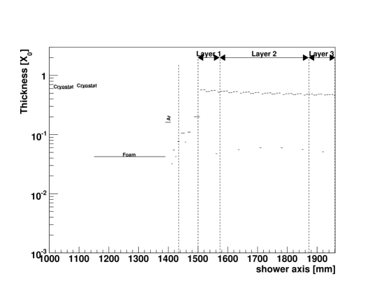
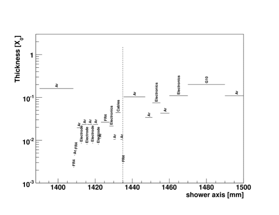
Figure 5: a) Amount of material in the beam line starting just before the cryostat along the axis of a particle penetrating at $\eta=0.687$. b) Detailed view of the material in the presampler and before the first compartment.

4 Electronic Calibration

The ionisation signal from the calorimeter is brought via cables in the LAr out of the cryostat to the front end crates (FEC). These crates, directly located on the cryostat, house both the Front End Boards (FEB) and the calibration boards.

On the FEB, the signal is first amplified by a current sensitive preamplifier. In order to accommodate the large dynamic range and to optimise the total noise (electronics and pile-up), the signal is shaped with a CR-RC² architecture (bipolar shape) and split in three linear scales with a typical ratio $1:9.2:92$, called low, medium and high gain. For a given channel these three signals are sampled at the $40$ MHz clock frequency and stored in an analog pipeline (Switched Capacitor Array) until the trigger decision. After a trigger, a predefined number of samples ($N$) is digitised by a $12$ bit ADC. This digitisation is done either on each gain or on the most suited gain according to a hardware gain selection based on the amplitude of a fixed sample in the medium gain.

The response dispersion of the electronics read-out is about $2$%. To account for such an effect and for the different detector capacitances of each calorimeter cell, the calibration board provides to all channels an exponential signal that mimics the calorimeter ionisation signal. This voltage signal is made by fast switching of a precise DC current flowing into an inductor and is brought to the motherboard on the calorimeter via a $50$ $\Omega$ cable terminated at both ends. The amplitude uniformity dispersion is better than $0.2\%$. One calibration signal is distributed through precise resistors to $8$ ($32$) calorimeter cells for the middle (front and back) compartment whose location is chosen such that cross-talk can be studied.

Details on the calibration of the electronics can be found in Ref. [11]. Here we summarise those aspects which are relevant for the linearity of the energy measurement.

The cell energy is reconstructed from the measured cell signal using:

$$E^{vis}_{cell}=\frac{1}{f_{I/E}}\;F_{gain}\;\sum_{sample=1,N}OF_{sample,gain}\;(S_{sample}-P_{gain}),$$ (1)

where $S_{sample}$ is the signal measured in ADC counts in $N$ time slices, $P_{gain}$ is the pedestal for each gain (see section 4.1) and $OF_{sample,gain}$ are the optimal filtering (OF) coefficients derived from the shape of the physics pulse and the noise (see section 4.2). The function $F_{gain}$ converts for each gain ADC counts to currents in $\mu A$ (see section 4.3). The factor $f_{I/E}$ takes into account the conversion from the measured current to the energy (see section 4.4).

4.1 Pedestal Subtraction

In order to determine the signal levels where no energy is deposited in the detector, special runs with random triggers and no beam were taken (”pedestal runs”). The stability of the pedestal values was checked using runs taken in regular intervals throughout the data taking period. A run-by-run instability was observed in particular for the PS which has a non-negligible effect on the reconstructed energy. No instability has been observed within a run. To minimize the effects of such instabilities each electron run was corrected using pedestal values measured with random triggers within the same run. This ensured that for each physics run the correct pedestals are calculated and possible biases of about $20$ MeV are corrected.

4.2 Determination of the Signal Amplitude

The peak amplitude $A$ (and the signal time) is extracted from the $N=5$ signal samples ($S_{sample}$) using a digital filtering technique [12]. The peak amplitude is expanded in a linear weighted sum of coefficients (OF) and the pedestal subtracted signal in each sample (see eq. 1).

The coefficients are calculated using the expected shape of the physics signal, its derivative and the noise autocorrelation function. The noise contribution is minimised respecting constraints on the signal amplitude and its time jitter. The noise autocorrelation function is determined from randomly triggered events.

The shape of the physics signal can be predicted using a formula with four free parameters that can be extracted from a fit to the measured physics pulse shape [13]. For each cell, the OF coefficients are then calculated [14]. Over the full module, the shapes of the measured and predicted physics pulse agree to within $2\%$ and the residuals of the pulse shape at the peak position are within $0.5$% in the first and $1$% in the second compartment. For the cells involved in the electron energy measured at the beam position studied in this analysis, the residuals deviate by at most $7\cdot 10^{-3}$ in the first compartment and by at most $2.5\cdot 10^{-3}$ in the second compartment.

Due to the fine segmentation of the first calorimeter compartment there is unavoidably a capacitive coupling between the read-out cells (strips). This cross-talk affects the signal reconstruction during the calibration procedure as well as the physics pulse shapes. The cross-talk (see section 4.3) has been taken into account in the determination of the OF coefficients.

4.3 Calibration of the Read-out Electronics

The relation between the current in a LAr cell ($\mu A$) and the signal measured with the read-out electronics (in ADC counts) is determined by injecting with the calibration system a well known current. Calibration runs have been taken in regular intervals (about every $12$ hours) for each cell. In these calibration runs currents with linearly rising amplitudes (in DAC units) are injected (”ramp runs”).

For each cell and for each injected current, the amplitude is reconstructed from the measured signal (after subtracting a parasitic injected current) adjusting the pulse shape derived from special calibration runs (“delay runs”), where a signal with a fixed amplitude and a variable time for the pulse is injected.

Each reconstructed amplitude rises almost linearly with the input signal. To correct for small non-linearities the dependence of the reconstructed amplitude on the input signal is fitted with a fourth order polynomial. This fit is used to reconstruct the visible energy in a LAr cell ($F_{gain}$ in eq. 1).

As an example, in Fig. 6 the results of the ramp run analysis is shown for the cell that had on average the largest energy fraction during the data taking period. The relation between the injected current in $\mu A$ and the reconstructed amplitude in GeV is shown. For a given DAC value on the calibration board a current is injected and the resulting signal is measured in ADC counts. To facilitate the interpretation the data are already transformed into in GeV units.

The data obtained in medium gain are shown as open circles. Data in high gain are shown as closed circles. At low energies, where the signal can be reconstructed in both gains good agreement is found. In the region where the gains are switched the difference between the high gain and the medium gain is only a few MeV. The deviation from linearity of the electronics for a cell signal is $1-2\%$. The line shows the result of a fit of a fourth order polynomial $P_{4}({\rm ADC})$. The bottom part of the figure shows the residuals, i.e., the difference between the reconstructed and the input signals in MeV. For the medium (high) gain the signal is reconstructed with an accuracy of $40$ ($10$) MeV.

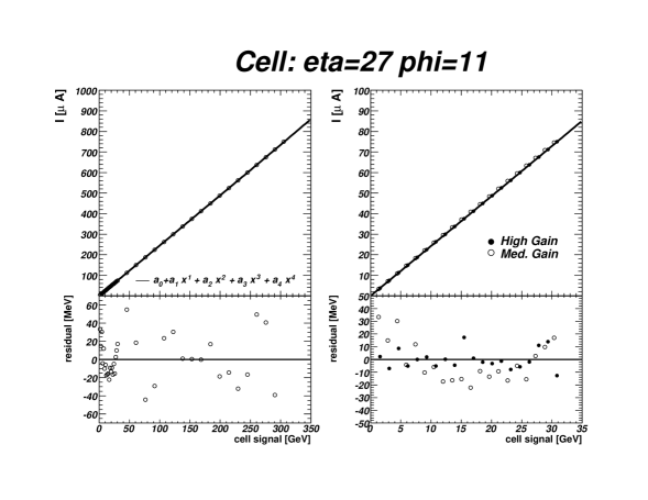
Figure 6: Relation of the measured cell signal in GeV and the current ($\mu A$) injected by the calibration system for high and medium gain. Superimposed is the result of a fit to a fourth order polynomial. In the bottom the residual, the difference of the injected current and the fit, is shown as a function of the measured signal. In a) the results for the medium gain and in b) the results for the high gain are shown. In addition, in b) the low signals of the medium gain are superimposed.

During the calibration of the electronics the cells are pulsed with a pattern where between two pulsed cells three cells are not pulsed. Since the calibration constants are derived from the known injected current and the measured signal for the pulsed cells, they are overestimated if the effect of cross-talk is not taken into account. In the first compartment, where the capacitive coupling between the cells is large, a cross-talk correction is derived for each cell using delay runs. It is obtained by adding the signal measured in the two closest passive neighbours of pulsed cell and the average of the next-to-closest neighbour. The correction factors do not strongly vary for different electronic gains and they are moreover stable for all pulse values.

4.4 The Current to Energy Conversion Factor

The conversion from the measured current ($\mu{\rm A}$) to the visible energy ( MeV) is done using a factor $f_{I/E}$, which is assumed to be independent of the beam energy. There is one common factor for the three accordion compartments and one factor for the presampler. Both factors are difficult to calculate from first principles. The difficulties arise from the complex structure of the electric field and from the modelling of physical effects like recombination of electrons in the LAr.

In this analysis they are determined from a comparison of the visible energies in the data and in the Monte Carlo simulation, where the complex accordion geometry and in particular the electrical field are simulated in detail. In this way also the dependence of the simulated signal on the range cut, below which a particle is not tracked any further and deposits all its energy, is absorbed. Since the current to energy conversion drops out in the linearity analysis, its exact value is not critical.

The $f_{I/E}$ factor can be roughly estimated using a simplified model, where a detector cell is seen as a capacitor with constant electrical field: $f_{I/E}=e/(w*t)\approx 15$ nA/MeV, where $e$ is the elementary charge, $w$ is the ionisation potential of LAr and $t$ is the drift time. The comparison of the data to the Monte Carlo simulation gives in the accordion calorimeter $f_{I/E}=16.0$ nA/MeV.

The calibration signal amplitude is attenuated due to the skin effect in the cables. The different lengths used in each compartment result in a small bias and the front signal has to be corrected by a factor $1.007$. Differences from the slightly different electrical fields in the first and the second compartment (due to the different bending of the accordion folds) are estimated to be of the order of $0.3\%$ (using calculations of the electric field). The cross-talk effect in the first compartment (see section 4.3) is corrected cell-by-cell. The result of this correction is that on average the measured total signal is lowered by a factor $0.93$. For all these effects, an uncertainty of $\pm 0.5\%$ is assigned for the relative normalisation of the first and the second compartment.

In addition, a correction for cross-talk between the second and the third compartment is also needed. This is due to the read-out lines of the second compartment passing through the third one. Empirically it has been found that $0.55\%$ of the energy deposited in the second compartment ($E_{2}$) is measured in the third compartment ($E_{3}$). Therefore, $0.55\%$ of $E_{2}$ is subtracted from $E_{3}$ and added to $E_{2}$. The overall energy is not changed by this correction. However, to compare the energy fraction deposited in the individual layers and the mean shower depth in data and Monte Carlo simulations it has to be taken into account.

In the PS the current to energy conversion factor is also estimated to be about $f_{I/E}=16$ nA/MeV. Two effects must be taken into account that reduce this factor: First, one cell with coherent noise had to be excluded from the analysis. For the impact point studied here this leads to a reduction of $0.95$ of the total PS signal (according to the Monte Carlo simulation). Second, the effective length of the PS is reduced to $11$ mm due to the vanishing electric field at the edges, the factor is $f_{I/E}=16\cdot(11/13)\cdot 0.95=12.9$ nA/MeV. This is in agreement with the number found from the comparison of data to Monte Carlo.

5 Calibration of Electromagnetic Showers

5.1 Calibration Constants for Sampling Calorimeters

In a sampling calorimeter the total deposited EM energy ($E^{tot}$) can be estimated from the energy deposited in the active medium ($E^{act}$) by dividing by the sampling fraction $f_{\rm samp}^{\rm e}$:

$$E^{tot}=\frac{1}{\mbox{$f_{\rm samp}^{\rm e}$}~{}}\;E^{act},\;\;{\rm with}\;\;\mbox{$f_{\rm samp}^{\rm e}$}~{}=\frac{E^{act}}{E^{act}+E^{pas}},$$ (2)

where $E^{pas}$ is the energy deposited in the passive material.

For a minimum ionising particle the sampling fraction is a fixed number which can be calculated from the known energy deposits in the active and passive materials due to ionisation. Since the energy loss of electrons is different from that of muons, the sampling fraction for electron is lower.

In Fig. 7a is shown the shape of the deposited energy distribution of an EM shower along the shower axis ($l$) for electrons with $E=10$ GeV, $E=100$ GeV and $E=500$ GeV, and for muons with $E=10$ GeV. The accordion calorimeter starts at $1500$ mm. The sampling structure of the calorimeter ends at about $1960$ mm. The energy depositions before and after the calorimeter are not shown.

The muon loses only a small part of its energy in the calorimeter. The dips approximately every $40$ mm are due to the lead traversed by the muon going through the accordion (zig-zag) folds.

While the energy deposited by muons is approximately constant, for EM showers the deposited energy rises quickly to a maximum and then is slowly attenuated. As the energy of the impinging particle increases, the shower penetrates deeper into the calorimeter. In most events the shower is contained inside the calorimeter and only a very small fraction of the energy leaks out. At the end of the shower more and more particles at low energy are produced.

Particles produced in the EM shower interact differently with the detector at the beginning and at the end of the shower development. At the end of the shower a large number of low-energetic photons are produced, which have a higher probablity to produce low energy electrons (via e.g. the photo-electric effect and Compton scattering) in the lead absorber than in the Lar. Since the range of these electrons is typically smaller than the lead absorber thickness, the energy deposit in the absorber increases relative to the energy deposit in the active material towards the end of the shower and the sampling fraction decreases [6, 15, 16, 17, 18, 19]. This is illustrated in Fig. 7b, where the sampling fraction along the shower axis is shown for the same particles as in Fig. 7a. While the sampling fraction is constant for muons, for electrons the sampling fraction decreases towards the end of the shower. For an electron with $E=10$ GeV the sampling fraction drops by $20$%. This behaviour depends on the electron energy. However, when the sampling fraction is calculated as a function of the relative distance from the shower maximum, it shows a universal behaviour, i.e., it does not depend on the electron energy [6] (see Fig. 7c).

When looking at a fixed point of the calorimeter, the sampling fraction can be different event-by-event due to longitudinal shower fluctuations. If, however, the response of the calorimeter is equal in all regions, the sampling fraction is the same when integrated over the whole shower depth. Therefore the calorimeter is linear. Nevertheless, a non-linearity is introduced, if only a part of the shower is contained in the calorimeter or if the longitudinal compartments are not equally calibrated, i.e., if they react differently to minimum ionising particles. In most practical applications, the shower starts already upstream of the calorimeter and a fraction of its energy is also deposited behind the calorimeter. This introduces an intrinsic non-linearity of the energy response due to longitudinal shower fluctuations, which must be corrected.

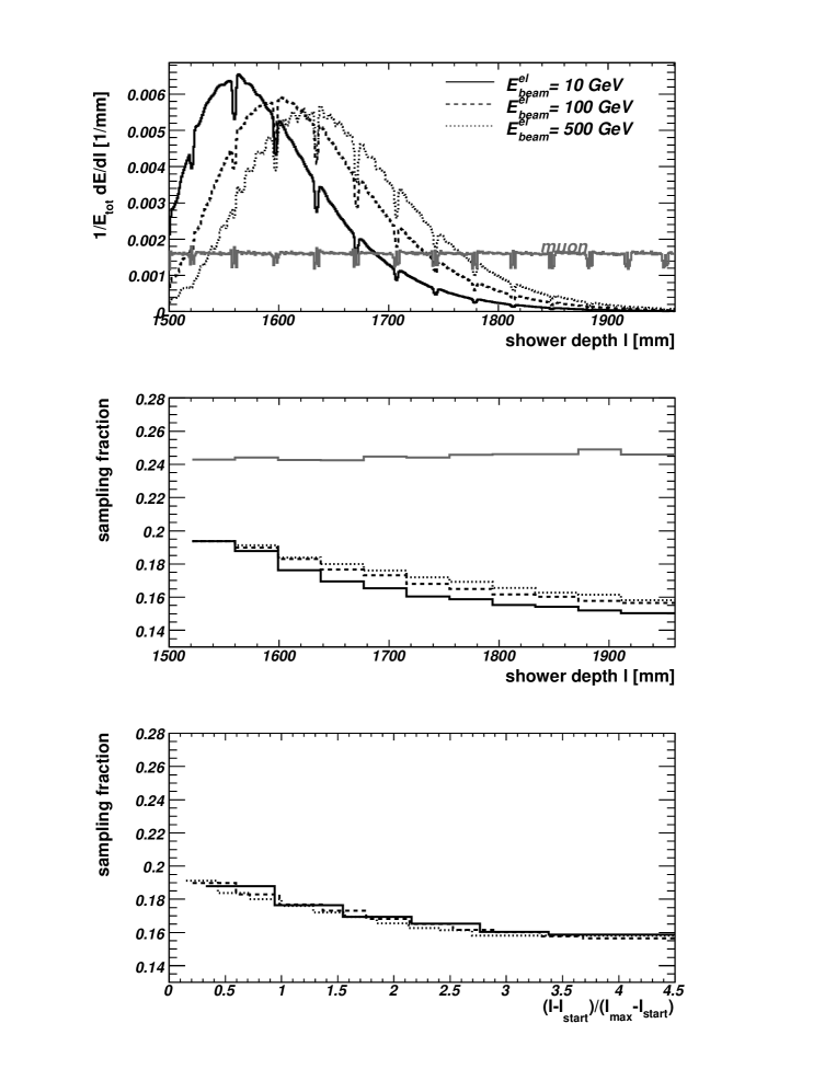
Figure 7: a) Shape of the energy deposited along the shower axis. b) Sampling fraction along the shower axis. c) Sampling fraction rescaled to the shower maximum. Shown are Monte Carlo simulations for electrons with beam energies of $10$, $100$ GeV and $500$ GeV and muons with $10$ GeV. In c) $l_{start}$ is defined as the beginning of the calorimeter and $l_{max}$ is the maximum of the shower.

5.2 Correction for Upstream Energy Losses using Presampler Detectors

The principle of a presampler detector is that the energy deposited in a thin active medium is proportional to the energy lost in the passive medium in front of the calorimeter. The difference with respect to a sampling calorimeter is that the passive material, the “absorber”, is very thick, typically about $1-2$ $X_{0}$, and that there is only one layer of passive and active material. Therefore, the calibration scheme is different from the one of sampling calorimeters where a shower passing a radiation length is sampled many times.

If an electron passes through the passive material in front of the presampler, it continuously loses energy by ionisation. The total deposited energy in the passive material is approximately constant and can be calculated assuming the energy is lost by a minimally ionising particle. However, the electron also emits photons by Bremsstrahlung. Depending on their energy they either react through Compton scattering or photo-electric effect (in this case their energy is mainly deposited in the dead material by low energy electrons) or they do not interact until they create an electron positron ($e^{+}e^{-}$) pair. The pair can be produced in the passive material, in the active medium of the presampler or in the sampling calorimeter. In the latter case, their energy is simply measured in the calorimeter and nothing has to be done in addition. The energy deposited by each particle of the $e^{+}e^{-}$ pair is therefore in many cases smaller than the energy deposited by the beam electron passing through the full passive material. In the case where the pair is created in the presampler itself, the energy measured in the presampler is even largely uncorrelated to the energy deposited in the passive material.

In any case the electrons produced by pair-production will traverse none or part of the passive material. If one $e^{+}e^{-}$-pair is created in the passive material, three electrons ionise the active medium. Two of them have only traversed a small part of the passive material. The correct calibration constant is therefore smaller than the one calculated from the inverse sampling fraction of a minimum ionising particles.

The total energy deposited in the active and in the passive material in and before the presampler $E^{tot}_{0}$ can be reconstructed from:

$$E^{tot}_{0}\;\;=w_{PS}\;E^{act}_{0}\;\;=\frac{a+b\;E^{act}_{0}}{E^{act}_{0}}\;\;E^{act}_{0}=a+b\;E^{act}_{0}$$ (3)

where $E^{act}_{0}$ is the energy deposited in the active medium of the presampler. The calibration coefficient $a$ represents the average energy lost by ionisation by the beam electron. Its energy dependence might be caused by low energy photons produced by Bremsstrahlung that are absorbed in the dead material and by photon nucleon interactions. The amplification factor $b$ takes into account that the $e^{+}e^{-}$-pairs produced in the passive material or in the active medium have only traversed part or none of the material in front of or in the PS.

The calibration factors depend on the details of the experimental set-up and have to be extracted from a Monte Carlo simulation.

6 Electron Energy Reconstruction

6.1 Reconstruction of the Electron Cluster Energy

When an electron penetrates the ATLAS calorimeter a compact EM shower is developed, which deposits most of the energy near the shower axis. To reconstruct the electron energy, the energies deposited in a fixed number of calorimeter cells are added together. No noise cut is applied. This collection of cells is called “cluster”. Since the radial EM shower energy profile depends merely on the electron energy, the signal loss from cells outside the cluster can be easily corrected.

The electron cluster is constructed from the second accordion compartment, where all cells within a square of $3{\rm x}3$ cells around the cell with the highest energy are merged. For the other accordion compartments all cells which intersect the geometrical projection of this square are included. In the first accordion compartment, which has high granularity in the $\eta$-direction, $8$ cells from each side of the cell with the maximum energy in this compartment are added to the cluster. For the impact point analysed here, two cells in $\phi$ are included. Thus, a cluster includes $17{\rm x}2$ cells in the first, $3{\rm x}3$ cells in the second and $2{\rm x}3$ in the third compartment. while in the PS $3{\rm x}2$ cells are used to define the visible energy.

To reconstruct the electron energy deposited in the accordion calorimeter the visible energy measured within the electron cluster defined above is multiplied by a calibration factor:

$$E^{rec}_{acc}=\sum_{i=1,3}E^{rec}_{i}=\frac{1}{d(E)\,\scriptsize f_{samp}}\;\sum_{i=1,3}E^{vis}_{i},$$ (4)

where $E^{vis}_{i}$ is the visible energy in the $ith$ compartment and $f_{samp}=0.18$ is the sampling fraction taken for an electron with an energy of $100$ GeV (see eq. 2).

The factor $d$ is depends on the initial electron energy (see Fig. 8c). Its variation is mainly (about $0.6$%) due to the decrease of the sampling fraction towards the end of the shower, and due to the fact that the shower has already started before entering the accordion calorimeter as discussed in section 5.1. In addition, the factor $d$ corrects for a drop of the total energy of about $10$% due to the reduced charge collection near the accordion folds and for energy lost laterally (typically $4$% of the total electron energy). The fraction of energy outside the electron cluster varies by about $0.3$% with energy. The current to energy conversion leads to a decrease of the reconstructed energy by $0.5$% at high energies. Since these effects are correlated, they do not factorise and are therefore absorbed into one factor.

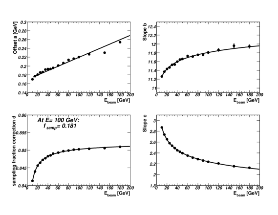
Figure 8: Calibration parameters extracted from the Monte Carlo simulation as a function of the beam energy. The calibration parameters are defined in eq. 7. The lines illustrate a parameterisation of the energy dependence of the calibration coefficients.

6.2 Correction for Upstream Energy Losses

Following the correction procedure for energy losses in the upstream material, described in section 5.2, the total energy deposited in and before the PS is reconstructed by:

$$E^{rec}_{0}=a+b\;E^{vis}_{0},$$ (5)

where $E^{vis}_{0}$ is the visible energy in the PS cluster.

The calibration parameters $a$ and $b$ are obtained from the Monte Carlo simulation. As an example, the correlation between the visible energy deposited in the PS and the true energy deposited upstream and in the PS is shown in Fig. 9a and Fig. 9b for electrons with $E=10$ and $E=180$ GeV. The calibration parameters $a$ and $b$ are determined by a linear fit.

The offset $a$ rises linearly with the beam energy (see Fig. 8a) and can be easily parameterised. The slope $b$ rises logarithmically (see Fig. 8b)). The value of $b$ corresponds to about $60\%$ of the inverse sampling fraction of a minimally ionising particle completely passing through the full active and passive medium.

6.3 Correction for Energy Losses between the Presampler and the Accordion

The region between the PS and the first accordion compartment contains support structures, electronics and cables. The amount of passive material depends on the impact point in $\eta$ and $\phi$.

At this point, a muon with an energy of $10$ GeV deposits $0.6$% of its energy in the passive material in front of the calorimeter and about $0.15$% in the passive material between the PS and the first accordion compartment. However, electrons deposit a larger fraction of their energy in the material between the PS and the first accordion compartment. An electron with $10$ GeV deposits on average $3.6$% of its energy in the passive material in front of the calorimeter and $4.1$% in the passive material between the PS and the first accordion compartment. The fact that more energy is deposited behind the PS than before gets more pronounced towards higher energies. An electron with $180$ GeV deposits $0.45$% of its energy in the passive material in front of the calorimeter and $0.85$% in the passive material between the PS and the first accordion compartment.

The energies deposited before and just after the PS are linked via the dynamical behaviour of the EM shower development. According to the Monte Carlo simulation, a good correlation to the energy deposited between the PS and the first accordion compartment can be obtained from an observable combining the energy in the PS and the energy measured in the first accordion compartment, namely:

$$E^{rec}_{PS/Strip}=c\;{(E^{vis}_{0}\cdot E^{vis}_{1})}^{0.5}.$$ (6)

The value of the exponent in eq. 6 has been found empirically. The calibration coefficient $c$ is obtained from the Monte Carlo simulation. The result of the simulation is shown in Fig. 8d) as a function of the beam energy.

As an example, the correlation between ${(E^{vis}_{0}\cdot E^{vis}_{1})}^{0.5}$ and the true energy deposited between the PS and the first compartment is shown in Fig. 9c and Fig. 9d for electrons with $E=10$ and $E=180$ GeV. The calibration parameter $c$ is obtained as the slope of a linear fit. While this assumption is justified for low energies, at high energies deviations from a linear correlation are observed. The exponent in eq. 6 seems to be slightly energy dependent. Since, however, the dead material correction is less important at high energies, within the present accuracy this effect can be neglected.

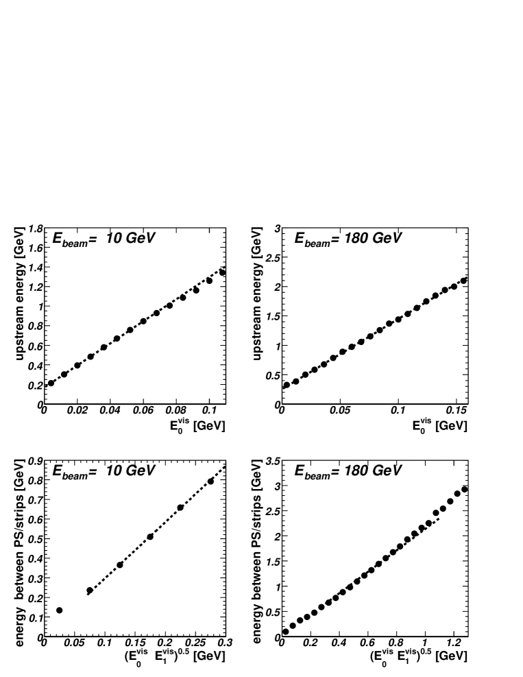
Figure 9: Mean energy lost before and in the PS as a function of the visible energy in the PS for electrons of $10$ (a) and $180$ GeV (b). Mean energy lost after the PS and before the first accordion compartment as a function of the estimator $(E^{vis}_{0}\cdot E^{vis}_{1})^{0.5}$ for electrons of $10$ (c) and $180$ GeV (d). The dashed lines indicate the linear approximation in the range, where the calibration parameters have been extracted.

6.4 Correction for Downstream Energy Losses

In the region analysed in this study, i.e. $\eta=0.687$, the electron passes materials with a total thickness of about $30$ $X_{0}$. Therefore the energy fraction leaking out behind the calorimeter is small.

The amount of energy leaking out of the back of the calorimeter can be determined from the Monte Carlo simulation. On average, about $0.35$% of the initial electron energy with $E=10$ GeV is deposited behind the calorimeter, increasing linearly to $0.45$% for $E=245$ GeV. Thus, the longitudinal energy leakage introduces a non-linearity of about $0.1$% in this energy range.

This effect is corrected on average for each energy point.

6.5 Correction for the Impact Position within a Cell

Due to the complex structure of the accordion folds, the energy response changes as a function of the $\phi$ position of the impinging particle within a cell. The main reasons are the varying amount of passive absorber material and changes in the electric fields. In the $\eta$-direction, a drop of the measured energy is observed, if the electron does not impinge on the cell centre. This effect is due to an incomplete containment of the electron in the cluster. These effects have been already reported in Ref. [11].

The electron $\phi$ impact position within a cell is reconstructed from the energy weighted barycentre of the second layer. The bias due to the finite calorimeter cell size is corrected using the average difference of the position measurements provided by the calorimeter and by the beam chamber measured as a function of calorimeter position measurement (“S-shape”). The corrected $\Phi$ impact position normalised to middle cell units is called $\Phi_{calo}^{corr}$.

The meassured dependence of the mean energy on $\Phi_{calo}^{corr}$ is shown in Fig. 10 for an electron beam energy of $E=100\mbox{\rm~{}GeV}$. The peak-to-peak modulation for different impact positions is about $1.5\%$. The modulation is parameterised with a function with eight free parameters having a sinusoidal term correcting for the accordion structure and a parabola term correcting cluster containment effects. The form of the adjustment is shown in Fig. 10 as line.

The correction is obtained from the data run with an electron beam energy of $100$ GeV, where the largest data sample was available, and is applied to all other energies.

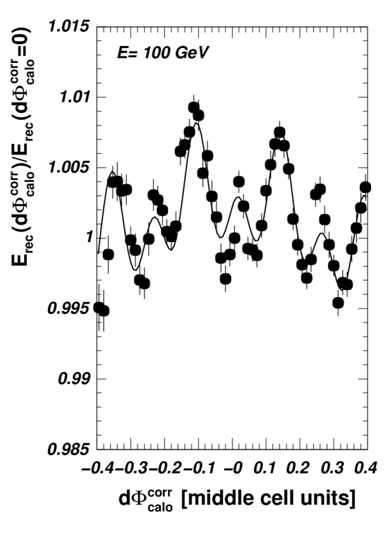
Figure 10: Correction for the mean energy as a function of the $\phi$ impact position within a cell obtained from a data run with electrons at $E=100$ GeV. Overlayed as line is a parameterisation.

6.6 Corrections for Bremsstrahlung Photons lost in the Beam-line

Photons produced by Bremsstrahlung of the beam electron in the passive material before the last trimming magnets, $40$ to $170$ m upstream of the detector, cannot reach the calorimeter. Therefore a correction has to be applied to the electron energy measured by the calorimeter.

The amount of material in this region associated with the NA45 experiment is not well known and has to be estimated. In the beam-line, there is about $0.03$ $X_{0}$ of air, and about $0.01$ $X_{0}$ of material from the beam pipe windows. In the Monte Carlo simulation this “far” material is modelled by a thin spherical shell of Aluminium. Since the energy lost by Bremsstrahlung leads to a tail on the low energy side of the reconstructed energy distribution, the amount of material can be estimated by comparing the tails of the reconstructed energy distribution in Monte Carlo simulations with different amounts of material and in the data at various beam energies. An aluminium thickness of $0.04\pm 0.01$ $X_{0}$ has been estimated in this manner.

The particles produced by Bremsstrahlung in the ”far material” are not tracked any further in the simulation, but their total energy is recorded. The correction can then be estimated by looking at the reconstructed energy with and without the lost energy added to the measured calorimeter energy.

If the photon energy is relatively large, the electron energy can be considerably lower than the original beam electron. Since the beam optics is optimised for electrons with the nominal beam energy, there is a certain probability that the electron will not reach the scintillator S3 and S4 defining the beam spot. This effect has been evaluated using a simulation of the beam-line based on the TURTLE program[20]. At a beam energy of $10$ GeV, for an electron having lost $1\%$, $5\%$ or $10\%$ of its energy, only for $98\%$, $77\%$ and $50\%$ of the events the electron arrives in the calorimeter. For a beam energy of $50$ GeV, the corresponding probabilities are $100\%$, $86\%$ and $56\%$. This correction is applied to the Monte Carlo simulation as an event weight for each measured distribution.

The correction due to Bremsstrahlung is shown in Fig. 11. For an electron energy of $E=10$ GeV the peak of the reconstructed energy distribution is shifted by $0.25$%, at $E=50$ GeV by $0.15$%, and at $E=180$ GeV by $0.09$%. The non-linearity induced by Bremsstrahlung in the “far” material is therefore about $0.2$% before correction.

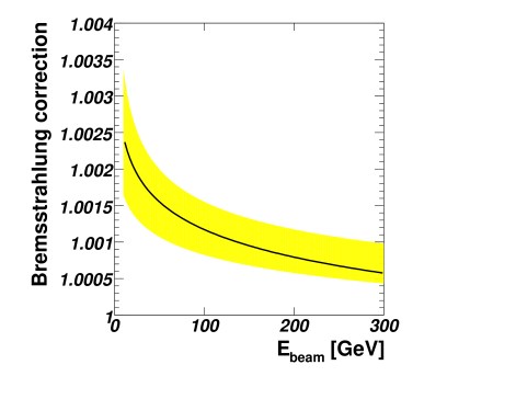
Figure 11: Correction for the effect of Bremsstrahlung in the “far” material as a function of the electron beam energy. The solid line indicates the correction for the standard beam-line set-up. The band gives the uncertainty due to variation of the “far” material.

6.7 The Final Electron Calibration Scheme

The final electron calibration scheme is a sum of the individual corrections described above:

$$E^{rec}=\left(a(E)+b(E)\;E^{vis}_{0}+c(E)\;(E^{vis}_{0}\cdot E^{vis}_{1})^{0.5}+\frac{1}{d(E)\,f_{samp}}\;\sum_{i=1,3}E^{vis}_{i}\right)$$

$$\cdot f_{\rm cell\,impact}(\Delta\Phi)\cdot(1+f_{\rm leakage}(E)),\;\;\;\;\;\;\;\;\;\;\;\;\;\;\;\;$$ (7)

where $E^{vis}_{i}$ is the visible cluster energy deposited in the $i$th ($i=0,3$) calorimeter compartment, $f_{samp}=0.18$ is the sampling fraction for an electron with $E=100$ GeV and the functions $f$ correct (event-by-event) for the effect of longitudinal leakage ($f_{\rm leakage}$) (see section 6.4) and of the cell impact position ($f_{\rm cell\,impact}$) (see section 6.5). The mean reconstructed energy is in addition corrected for upstream Bremsstrahlung losses ($f_{\rm brems}$) (see section 6.6).

Since the calibration parameters slightly depend on the energy to be measured, an iterative procedure is needed to reconstruct the electron energy.

7 Comparison of Data and Monte Carlo Simulations

Since the calibration scheme described above is based on the Monte Carlo simulation, it is important to verify that the Monte Carlo simulation reproduces the total energy distribution, the energies measured in each layer and the lateral development of the EM shower.

The mean reconstructed energy in the PS and in the first and second compartment of the accordion is described by the Monte Carlo simulation for all energies within $\pm 2\%$. In addition, also the shape of the energy distributions within each compartment are well described. As an example, the shapes of the visible energy fraction distributions are shown in Fig. 12 for $E=10$ and $E=100$ GeV.

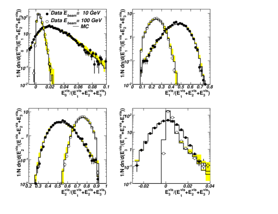
Figure 12: Visible energy fraction distribution for electrons with $E=10$ GeV and $E=100$ GeV in the PS (a) and the first (b), second (c) and third (d) compartment of the accordion calorimeter. Shown are data (circles) and a Monte Carlo simulation (line). The band indicates the uncertainty in the Monte Carlo simulation due to the “far” material and the material in front of the PS.

The distribution of the reconstructed total energy distribution is shown in Fig. 13 for electron beam energies of $10$, $50$, $100$ and $180$ GeV. The beam energy in the Monte Carlo simulation is scaled to the one in the data. The Monte Carlo simulation gives a good description of the data.

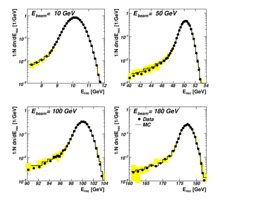
Figure 13: Shape of the reconstructed energy distribution for electrons with (a) $E=10$, (b) $50$, (c) $100$ and (d) $180$ GeV. Shown are data and a Monte Carlo simulation. The band indicates the uncertainty in the Monte Carlo simulation due to the “far” material and the material in front of the PS.

The shape of the energy distribution in the $\eta$-direction measured in the first compartment is shown in Fig. 14 for electron beam energies of $E=10$, $50$, $100$ and $E=180$ GeV. The $\eta$-position is calculated with respect to the shower barycentre in the first compartment and expressed in units of read-out cells. Due to the compactness of an EM shower the radial extension depends only slightly on the beam energy. The distribution is found to be asymmetric (see also in Ref. [21]). At low electron beam energies, the Monte Carlo simulation gives an excellent description of the data. In particular, the asymmetry is well reproduced. At high energies the data distribution is slightly broader than predicted by in the Monte Carlo simulation.

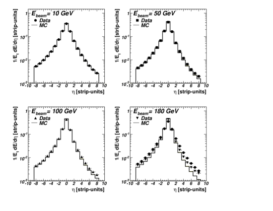
Figure 14: Shape of the energy distribution as a function of the $\eta$-direction in the first calorimeter compartment for beam energies of (a) $E=10$ GeV, (b) $60$ GeV, (c) $100$ GeVand (d) $180$ GeV. Shown are data (closed symbols) and a Monte Carlo simulation (lines). To illustrate the energy dependence the data with an beam energy of $E=10$ GeV are superimposed in d) to the data with $E=180$ GeV. The systematic uncertainty in the Monte Carlo simulation due to the “far” material and the material in front of the PS is shown, but is not visible.

In conclusion, the Monte Carlo simulation predictions are in good agreement with the shower development measured for the data.

8 Determination of the Pion Contamination using Monte Carlo Simulation

The instrumentation of the H8 beam-line used in the present analysis did not allow for a direct measurement of the pion contamination in the electron beam. Only the signal of the scintillator behind the calorimeter can be used to reject pions. The influence of a possible pion contamination has therefore to be estimated by comparing the electron and pion energy shapes predicted by the Monte Carlo simulation to the one measured in the data.

Since the LAr calorimeter has a thickness of about one interaction length, most pions deposit only a fraction of their incident energy. However, a small fraction of them can deposit most of their energy in the LAr calorimeter. For instance, at $E=10$ GeV about $3$% of the pions deposit more than $8$ GeV in the LAr calorimeter. Since these pions can influence the measurements of the electron energy, their fraction has to be determined.

Pions which deposit a lot of energy in the LAr calorimeter interact on average later in the LAr calorimeter than do electrons. Compared to electrons of the same beam energy they deposit therefore less energy in the first compartment and more in the second and third ones. The ratio $E_{1}^{vis}/(E_{2}^{vis}+E_{3}^{vis})$ is shown in Fig. 15a for $E=10\mbox{\rm~{}GeV}~{}$ and Fig. 15b for $E=50\mbox{\rm~{}GeV}~{}$ for data and an appropriate mixture of electrons and pions. The Monte Carlo simulation is able to describe the data. The fraction of pions in the electron beam is determined for each energy and varies from $2$% at $10$ GeV to $22$% at $180$ GeV. The effect on the electron energy measurement will be discussed in section 9.2.

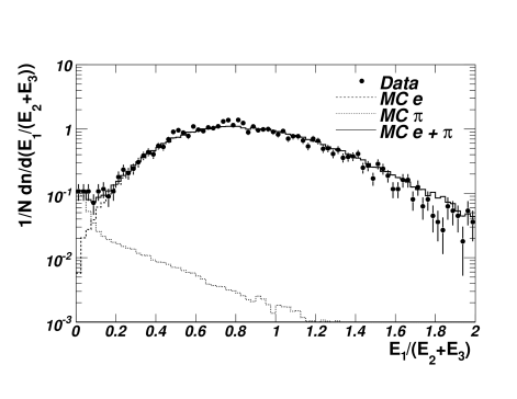
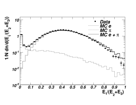
Figure 15: Shape of the ratio of the first ($E_{1}$) over the sum of the second ($E_{2}$) and of the third ($E_{3}$) calorimeter compartment. Shown are data (closed circles) with $E=10$ GeV (a) and $E=50$ GeV (b) and Monte Carlo simulations for electrons (dashed), pions (dotted) and an appropriate mixture of electrons and pions (solid).

9 Linearity and Resolution Results

9.1 Linearity Results

The mean energy is obtained by fitting a Gaussian to the reconstructed energy distribution within two standard deviations for the low energy side and three standard deviations for the high energy side. To determine the uncertainty due to the chosen fit range, results are also considered where the range of the low energy side is restricted to $1.5$ and extended to $2.5$ standard deviations.

The mean reconstructed energy divided by the beam energy is shown in Fig. 16. The error bars indicate the statistical uncertainty as obtained by the fit procedure. Since the absolute calibration of the beam energy is not precisely known, all points are normalised to the value measured at $E=100$ GeV. The inner band represents the uncorrelated uncertainty on the knowledge of the beam energy, while the outer band shows in addition the correlated uncertainty added in quadrature (see section 1). For energies $E>10$ GeV, all measured points are within $\pm 0.1$%. The point $E=10$ GeV is lower by $0.7$% with respect to the other measurements.

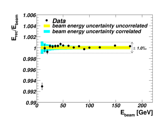
Figure 16: Ratio of the reconstructed electron energy to the beam energy as a function of the beam energy. All points are normalised to the value measured at $E=100$ GeV. The inner band illustrates the uncorrelated uncertainty of the beam energy measurement; in the outer band the correlated uncertainty is added in quadrature to the inner band.

9.2 Systematic Uncertainties on the Linearity Results

The systematic uncertainties induced by various effects on the reconstructed electron energy are shown in Fig. 17. In order to evaluate the size of some of the systematic uncertainties, dedicated Monte Carlo simulations have been produced to calculate new sets of calibration parameters. These samples were typically smaller than the default one.

The uncertainty on the current to energy conversion factor (see section 4.4) of the PS has been studied using the $\chi^{2}$-distribution of the visible energy distribution for data and Monte Carlo simulations for all energy points. The uncertainty is estimated by the scatter for different energies. The same procedure has been repeated by studying the dependence of the mean reconstructed energy on the PS energy in the data and in the Monte Carlo simulations. A consistent result has been found. Since the relative contribution for the PS is larger at low energies, the systematic uncertainty rises towards low energies (see Fig. 17a). While the systematic uncertainty is negligible at $E=180$ GeV, it reaches about $0.1$% at $E=10$ GeV.

The uncertainty due to the relative normalisation difference between the first and the second compartments (see section 4.4) is shown in Fig. 17b. This effect biases the energy measurement by up to about $0.1$%, mostly at low energies.

The systematic uncertainty arising from the incomplete knowledge of the amount of LAr between the PS and the LAr excluder in front of it (see section 3) is shown in Fig. 17c. It introduces an uncertainty of about $0.05$%. Again, low energies are most affected.

Fig. 17d shows the effect of adding ad hoc $0.02$ $X_{0}$ additional material between the PS and the first compartment. The relative variation of the reconstructed beam electron energy is slowly decreasing from low to high energies The effect amounts to about $0.1$% at low energies. At $E=10$ GeV even $0.2\%$ is found.

As explained in section 4, according to the amplitude of a predefined sample in the medium gain, a selection of the gain to be digitised is done. In the test-beam electrons arrive at any time with respect to the $25$ ns clock used by the data acquisition system. When this sample is not at the peak of the signal, it happens around the threshold that the cell is digitised in the high gain while it should have been done in the medium gain. The fraction of such events depends on the trigger phase with respect to the 40 MHz clock. Moreover, in the calibration procedure no continuity of the reconstructed amplitude near the overlap region of high and medium gain has been imposed. A combination of these two effects can induce a change of the reconstructed energy especially in the electron range from $40$ to $80$ GeV. This effect was studied by selecting events sampled near the peak ($10<t_{tdc}<20$ ns) and outside this time window ($t_{tdc}<10$ ns or $t_{tdc}>20$ ns). In ATLAS a timing adjustment will be performed such that the maximum sample is near the maximum of the signal, which corresponds to $15$ ns in the testbeam data taken in asynchronous mode. As shown in Fig. 17e, the largest effect is about $\pm 0.1\%$ at $60$ GeV.

The uncertainty introduced by restricting or extending the fit range of the Gaussian to the reconstructed energy distribution (see section 9.1) is shown in Fig. 17f. At low energies the uncertainty reaches $0.1$%, above $E>60$ GeV it is negligible.

The bias introduced by the uncertainty of the ”far” material and correspondingly of the Bremsstrahlung correction (see section 6.6) is shown in Fig. 17g. The resulting uncertainty is about $0.05\%$ (up to $0.1\%$ at two energies).

To test the influence of an incomplete description of the low energy tail laterally to the shower axis, the whole analysis is repeated using a $5{\rm x5}$ instead of a $3{\rm x3}$ cluster. The change with respect to the standard analysis is shown in Fig. 17h). The uncertainty is about $0.1\%$.

Fig. 17i) shows the effect of using different range cuts in the Monte Carlo simulation. The default value of $20$$\mu$m is decreased to $10$$\mu$m and increased to $100$$\mu$m. Although visible energy and sampling fraction significantly change in the Monte Carlo simulation, the linearity remains constant within about $0.05\%$ ($0.1\%$ in exceptional cases).

In the default Monte Carlo the small deformation of the calorimeter cells in the gravitational field of the earth is modeled (”sagging”). This effect introduces at most a change of $0.05\%$.

In an electromagnetic shower hadronic interactions of mainly photons with nucleons can lead to deposited energy that can not be measured in the calorimeter (nuclear excitation etc.) or can produce particles that escape detection (neutron, neutrinos etc.). According to the Monte Carlo simulation on average about $0.4$% of the energy can not be measured in the calorimeter. However, the energy dependence of this effect is small. While at high energies the relative variation of a Monte Carlo simulation with photon nucleon interactions switched off to the default case is constant, at low energies it is about $0.995-0.999$. This is shown in Fig. 17j).

The correction for the modulation of the reconstructed energy on the $\phi$-impact position within a cell (needed to improve the energy resolution) does not change the mean reconstructed energy within $0.05\%$.

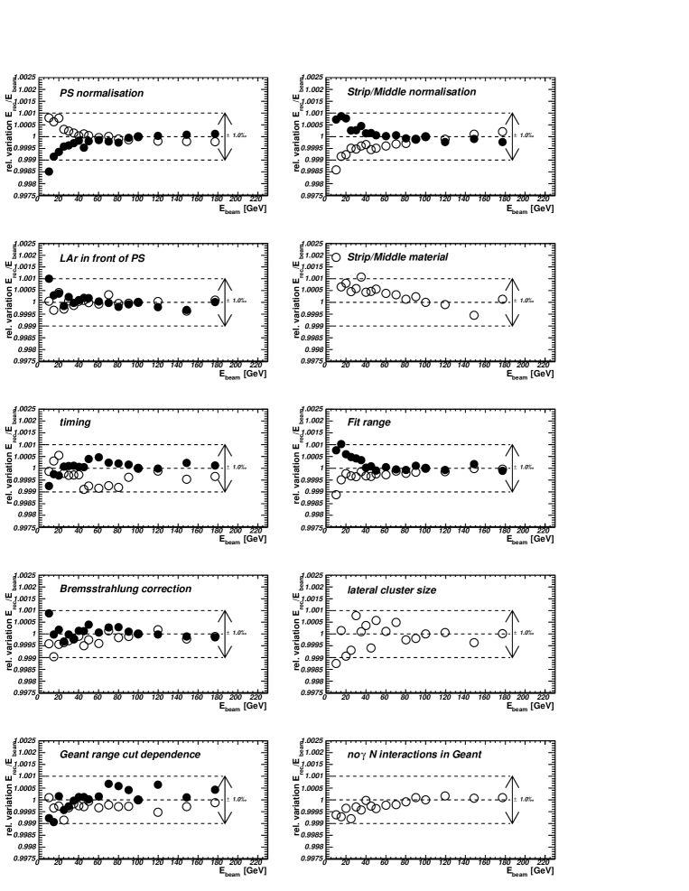
Figure 17: Sensitivity to systematic effects on the electron energy measurements: a) the normalisation of the PS, b) the relative normalisation of the strips and the middle, c) the amount of LAr in front of the PS, d) the amount of material between the PS and the strips e) the event arrival time with respect to the data acquisition clock, f) the range where the Gaussian fit is performed, g) the Bremsstrahlung correction (amount of ”far” material), h) the lateral shower description, i) the dependence on the range cut used in the simulation j) the presence of photon nucleon reactions in the simulation, Shown is the relative variation of the reconstructed to the beam electron energy. All points are normalised to the value measured at $E=100\mbox{\rm~{}GeV}$. The closed and open circles show the variations of the corresponding systematic uncertainties (see text) relative to the default.

To estimate how the reconstructed electron energy is biased by a possible pion contamination, the fraction of pions with a large energy deposit in the LAr is determined from the Monte Carlo simulation (see section 8) and the shift of the reconstructed mean electron energy in the Monte Carlo simulation is calculated. The shift is negligible at all energies.

In addition, data events with $E_{1}^{vis}/(E_{2}^{vis}+E_{3}^{vis})>0.1$ can be selected. Such a cut does not shift the reconstructed energy in the Monte Carlo simulation of electrons and does not change much the expected pion energy distribution. The reconstructed energy in the restricted data sample, where about half of the pions are expected to be removed, does not change.

To ensure a precise measurement of the electron energy, the energy dependence of the calibration parameters has to be taken into account. Since the initial electron energy is not known a-priori, an iterative procedure has to be applied. Starting from the measurement in the accordion calorimeter and using an average calibration parameter for the accordion calorimeter (parameter $d$ in eq. 7), the energy is reconstructed. With this first energy estimate, the calibration corrections are evaluated. This procedure is evaluated until the reconstructed energy does not change significantly. Already after two iterations an accuracy of better than $10^{-5}$ is achieved.

9.3 Interpretation of the Linearity Results

To quantify the non-linearity of the measured data points for $E>10\mbox{\rm~{}GeV}$, a first order polynomial is fitted. The resulting slope ($a_{1}$) is compatible with zero. When the analysis is repeated for each systematic uncertainty, slopes in the range $a_{1}=\pm 5\cdot 10^{-6}\mbox{\rm~{}GeV${}^{-1}$}$ are obtained. All systematic uncertainties combined in quadrature give an uncertainty of $\pm 9\cdot 10^{-6}\mbox{\rm~{}GeV${}^{-1}$}$. Based on purely statistical uncertainties, the $\chi^{2}$ per degree of freedoms for a linear fits to the data points is $\chi^{2}/ndf=2.7$. This, together with the fact that the pull distribution is not Gaussian (RMS is about 1.5), indicates that the measured data points are not fully compatible with a straight line and that systematic uncertainties affect the linearity.

In practical applications like the measurement of the $W^{\pm}$-boson mass, the shift of the measured (transverse) energy spectrum with respect to a reference reaction like that from the $Z^{0}$-boson needs to be understood. Since the transverse energy distribution is roughly peaked at half of the boson mass and slowly decreases towards lower transverse energies, one is interested in the control of the linearity within a few GeV. To estimate the size of local non-linearities for each energy measurement the local slope is calculated from the measurement which have a beam energy difference smaller than $20$ GeV. The result for the default measurement and for the systematic variations added in quadrature at each energy point (where the slope can be calculated) is shown in Fig. 18. In the region relevant for the measurement of the $\mbox{$W$}^{\pm}$-mass the local slope is known to a level of about $\pm 4\cdot 10^{-5}\mbox{\rm~{}GeV${}^{-1}$}$. This translates roughly to an uncertainty of $15$ MeV on the $\mbox{$W$}^{\pm}$-mass.

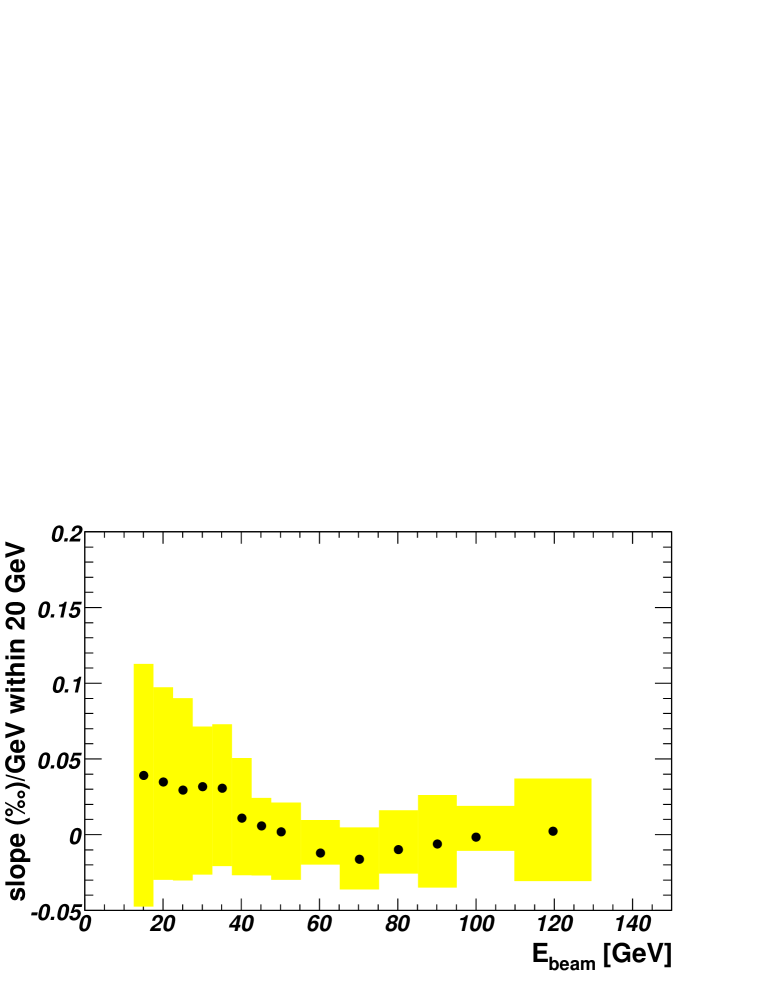
Figure 18: Slope calculated for the energy measurements within $20$ GeV around a given electron energy. The point represent the default result, while the band illustrates the slopes obtained from the systematic variations.

9.4 The Resolution Results

The energy resolution is obtained from the standard deviation of the Gaussian fit described in section 9.1. The relative resolution as a function of the electron beam energy is shown as closed circles in Fig. 19.

Since the noise depends on the electronic gain of the cells, the noise is subtracted for each energy point to obtain the intrinsic resolution of the calorimeter. The noise is evaluated as described in section 3. The noise is about $250$ MeV and slightly increases towards higher energies. The noise contribution to the resolution is shown in Fig. 19 as open squares. The data where the noise contribution and in addition the beam spread has been subtracted are shown in Fig. 19 as open circles. A function of the following form is fitted:

$$\frac{\sigma_{E}}{E}=\frac{a}{\sqrt{E}}\oplus b,\;{\rm with}\;a=10.1\pm 0.1\%\cdot\sqrt{\mbox{\rm~{}GeV}~{}}\;{\rm and}\;b=0.17\pm 0.04\%.$$ (8)

The symbol $\oplus$ indicates that the two terms are added in quadrature. The quoted errors are only statistical. The fit function is overlayed to the data points and gives a good description of the energy dependence in the data. The result is compatible with previous test-beam results taken in this $\eta$ region [11].

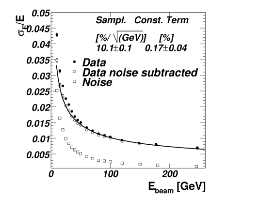
Figure 19: Fractional energy resolution as a function of the beam energy. Shown are the data before (closed circles) and after (open circle) the gain dependent noise subtraction. Overlayed as a line is a parameterisation of the resolution based on eq. 8 obtained from a fit. The open squares indicate the subtracted noise contribution.

Conclusions

Electron energy measurements with a module of the ATLAS electromagnetic barrel LAr calorimeter have been studied in the range from $10$ to $245$ GeV impinging at $\eta=0.687$ at the CERN H8 test-beam upgraded for precision momentum measurement. The beam energy has been monitored in the range $10<E<180$ GeV with an accuracy of $3\cdot 10^{-4}$ for the uncorrelated uncertainty and an uncertainty of $11$ MeV common to all energy points.

A calibration scheme has been developed for electrons that provides a good linearity and a good resolution at the same time. The mean reconstructed energy, the energy distributions, as well as the longitudinal and lateral energy profiles, are well described by the Monte Carlo simulation. Based on this simulation the data have been corrected for various effects involving the intrinsic non-linearities due to the varying sampling fraction, energy losses due to upstream and downstream interactions, energy depositions outside the electron cluster, and losses due to Bremsstrahlung at the beginning of the beam line.

In the energy range $15\leq E\leq 180$ GeV, the reconstructed energy response is linear within $\pm 0.1$%. The point at $E=10$ GeV is about $0.7\%$ lower than the other beam energies. At $E=245$ GeV no precise beam energy measurement was available.

The systematic uncertainties due to the limited knowledge of the test-beam or detector set-up or due to reconstruction effects is generally larger at low energies (up to about $\pm 0.1$%), but negligible at high energies. The non-linearity observed in the energy range of $40$ GeV and higher matches, if extendable to the whole calorimeter, the requirements for the $W^{\pm}$-mass measurement aiming for a precision of $15$ MeV.

The sampling term of the energy resolution is found to be $10\%\cdot\sqrt{\mbox{\rm~{}GeV}~{}}$, the local constant term is $0.17$%.

References

- [1] ATLAS Collab., ”Technical Design Report, Detector and Physics Performance”, CERN/LHCC/99-15 (May 1999).
- [2] ATLAS LAr Calorimeter Collab., ”Technical Design Report”, CERN/LHCC 96-41 (December 1996).
- [3] I. Efthymiopoulos, ”Evaluation of the bending power of the MBN spectrometer magnets of H8”, CERN SL/EA/IE internal note, Geneva (Switzerland) (March 2002).
- [4] A. Gustavson, ”Magnetic field measurements of the MBN magnets”, private communication (September 2002).
- [5] S. Hassani, These Universite Paris-Sud, LAL-02-89, Paris (France) (Sept. 2002).
- [6] G. Graziani, ”Linearity of the response to test beam electrons for the EM barrel module P13”, ATLAS internal note, ATL-COM-LARG-2004-001 (January 2004).
- [7] A. Asner, J. Vlogaert, ”Technical note on the MBN magnets”, CERN LAB-II/EA/note74-3, Geneva (Switzerland) (1974).
- [8] J. Loas, ”Mesure des premiers MBN”, CERN-SPS/EMA/note 77-7, Geneva (Switzerland) (1977).
- [9] B. Aubert et al., Construction, assembly and test of the Atlas electromagnetic barrel calorimeter, Nucl. Instrum. Meth. A 558 (2006) 388.
- [10] J. Agostinelli et al., Geant4: A simulation toolkit, Nucl. Instrum. Meth. A 506 (2003) 250.
- [11] B. Aubert et al., Performance of the Atlas electromagnetic calorimeter barrel module 0, Nucl. Instrum. Meth. A500 (2003) 202.
- [12] W. E. Cleland, E. G. Stern, Signal processing considered for liquid ionization calorimeter in a high rate enviroment, Nucl. Instrum. Meth. A 338 (1994) 467.
- [13] L. Neukermans, P. Perrodo, R. Zitoun, Understanding of the Atlas electromagnetic barrel pulse shape and the absolute e.m. calibration, ATLAS internal note, ATL-LARG-2001-008 (February 2001)
- [14] D. Prieur, ”Etalonnage du calorimètre électromagnétique du détecteur Atlas. Reconstruction des événements avec des photons non pointants dans le cadre d’un modèle supersymétrique GMSB”, These Université Annecy, LAPP-T-2005-03, Annecy (France) (April 2005).
- [15] K. Pinkau, Phys. Rev. 139 (1965) 1548.
- [16] H. Beck, Nucl. Instrum. Meth. 91 (1971) 525.
- [17] C. J. Crannell et al., Experimental determination of the transition effect in electromagnetic cascade showers, Phys. Rev. 182 (1969) 1435.
- [18] W. Flauger et al., Nucl. Instrum. Meth. A 241 (1985) 72.
- [19] J. del Peso, E. Ros, Monte carlo investigation of the transition effect, Nucl. Instrum. Meth. A295 (1990) 330.
- [20] D.C. Carey, K.L. Brown, Ch. Iselin, ”Decay TURTLE (Trace Unlimited Rays Through Lumped Elements) A computer program for simulating charged particle beam transport systems, including decay calculations”, SLAC Report No.246, Standford (USA) 1982, CERN 74-2, February 1974 Geneva (Switzerland), and NAL-64 December 1971.
- [21] J. Colas et al., Position resolution and particle identification with the Atlas em calorimeter, Nucl. Instrum. Meth. A550 (2005) 96.