Precision Calibration of the DØ HCAL in Run II

Abstract

Most of the physics analyses at a hadron collider rely on a precise measurement of the energy of jets in the final state. This requires a precise in situ calibration of the calorimeter with the final detector setup. We present the basic procedure and results of the in situ gain calibration of the D0 HCAL in Run II. The gain calibration works on top of the pulser-based calibration of the readout electronics and is based entirely on collision data.

1 Introduction

The detailed description of the DØ Calorimeter can be found in Run I and Run II instrumentation papers D0nimRunI ; D0nimRunII . Let us briefly summarize some of its basic aspects.

The DØ calorimeter is segmented into towers in $\eta$ and $\phi$. The precision towers divide the calorimeter in 64 segments in the $\phi$ and 72 segments in the $\eta$-direction. Each precision tower consists of four physical layers in the EM part and four or more physical layers in the hadronic part. The calorimeter is also divided into trigger towers, which are 2x2 arrays of precision towers, dividing the calorimeter into 32 segments in $\phi$, and 37 in $\eta$. Trigger towers are the smallest calorimeter units seen by the Level 1 trigger.

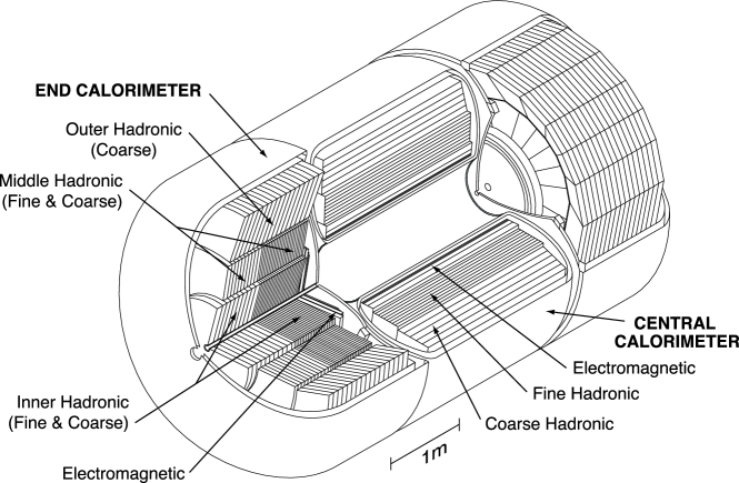
We distinguish a central section covering pseudorapidities $|\eta|$ up to $\approx 1.1$, and two end calorimeters (EC) that extend coverage to $|\eta|\approx 4.2$, with all three housed in separate cryostats, Fig.1. These are sampling LAr calorimeters with mainly Uranium absorber plates. A calorimeter basic unit consists of a 3 mm thick plate of an absorber material, 2.3 mm liquid Argon gap and a signal board consisting of a Copper pad surrounded by G10 insulator coated with high resistivity epoxy. The absorber is grounded and the pad is kept at positive voltage of 2000 V. Charge induced at the pads gives the physical signal. The electron drift time across the 2.3 mm gap is approximately 450 ns.

Figure 1: Isometric view of the DØ central and two end calorimeters in Run II.

Although for Run II the calorimeter itself is unchanged from Run I, the charge integration time has been reduced from $\sim$2.2 $\mu$s in Run I to $\sim$260 ns in Run II, resulting in an enhanced sensitivity to the finite mechanical precision of the calorimeter. Additional mechanical boundaries like module edges, any non-uniformities in the LAr gap and Uranium plate widths or possible board bendings are directly related to the amount of charge collected and the response of the modules and cells. In adittion, the associated readout electronics have been largely redesigned to address the need for a shorter shaping and readout time and the need for analog buffering to store the data until a Level 1 Trigger decision becomes available.

The Run II upgrade strongly influenced the calorimeter in an indirect way as well. The amount of dead material in front of the calorimeter increased significantly with the upgrade and it is non-uniformly distributed. This material comes from pre-shower detectors, the solenoid, fiber tracker and silicon vertex detector. Together with the cryostat walls the particles traverse at least of 3.7 $X_{0}$ before they reach the calorimeter. The amount of dead material depends also significantly on the angle of incidence of the measured particles and increases with the pseudo-rapidity.

Due to this significant changes for the upgrade, the calorimeter had to be calibrated again. Moreover, it was essential to obtain a calorimeter Run II calibration in situ with the final detector setup.

2 Calibration procedure

The calibration procedure for the DØ calorimeter contains two parts: calibration of the readout electronics using pulser data, and correction of non-uniformities due to mechanical variations in the detector using collision data.

The basic idea of the electronics calibration is to send a pulse of known charge into the readout, and to compare it to the measured charge. In this way we identify technical problems in the electronics, e.g. dead channels and correct for the channel-by-channel differences in the response. Pulses of different heights are used to probe the full dynamic range of every readout channel. In this way, the response of every single channel can be linearized, and the gains of the different channels can be equalized.

The gain calibration of the DØ calorimeter factorize into two parts: the calibration of the EM calorimeter and the calibration of the hadronic calorimeter. For this two parts of the calorimeter we determine the energy scale (i.e. a multiplicative correction factor), if possible per cell. Both parts of the calorimeter have been calibrated in two steps. First, the $\phi$-intercalibration to reduce the number of degrees of freedom, where special triggered Run II data was used. Second, the $\eta$-intercalibration to get access to the remaining degrees of freedom, as well as the absolute scale of the EM calorimeter. For the $\eta$-intercalibration we used $Z\to e^{+}e^{-}$ events for the EM calorimeter and QCD dijet events for the hadronic calorimeter.

The best standard candle for the absolute calibration of the EM calorimeter is the $Z$-peak, which is well known from LEP measurements. However, we lack of statistics to use the $Z$-peak alone in calibrating on a tower or cell level. Therefore we used special triggered EM data to intercalibrate over rings of fixed $\eta$. Once the $\phi$-degree of freedom is eliminated, the amount of $Z$ events is sufficiently high to absolutely calibrate each intercalibrated $\eta$-ring.

For this purpose the reconstructed $Z$ mass is written in terms of the electron energies and their opening angle. The electron energies are evaluated as the raw energy measurement from the calorimeter plus a parametrized energy-loss correction from a detailed detector simulation. Calibration constants are multiplicative to the raw cluster energy of each cell. A set of calibration constants is then determined that minimize the experimental resolution on the $Z$ mass and gives the correct LEP measured value. After the fully calibrated EM calorimeter, we address the calibration of the hadronic part.

3 $\phi$-intercalibration of the DØ HCAL

Due to the fact that the $p\bar{p}$ beams in the Tevatron are unpolarized, the energy flow in the direction transverse to the beam should not have any azimuthal dependence. Based on this, we can use an energy flow method with the following basic principle:

Consider in each case a given $\eta$-bin of the calorimeter. Measure the density of calorimeter objects above a given $E_{T}$ threshold as a function of $\phi$. With a perfect detector this density would be flat in $\phi$. Assuming that any $\phi$-non-uniformities are due to energy scale variations, the uniformity of the detector can be improved by applying multiplicative calibration factors to the energies of the calorimeter objects in each $\phi$-region in such a way that the candidate density becomes flat in $\phi$.

A special trigger was designed to record efficiently data for the hadronic $\phi$-intercalibration. It requires a transverse energy threshold of 5 GeV in the Trigger Tower at Level 1, then it requires at Level 2 that 5 GeV is in the hadronic part of the tower and finally it tightens the hadronic transverse energy cut for a Precision Tower at Level 3 to 7 GeV. Data for the $\phi$-intercalibration was taken during normal physics running. The quality of the recorded data was studied in detail to separate failures in redout electronics from gain miscalibrations. Systematic uncertainties from trigger non-unifomities were avoided by placing trigger and offline cuts sufficiently above the trigger conditions.

The task of deriving $\phi$-intercalibration constants for cells in towers at given $\eta$ is divided into the two following steps:

• Finding a tower calibration constant, which is a multiplicative factor for all cells in the tower, such that tower occupancies above an $E_{T}$ threshold are equalized in $\phi$.

• Fitting layer calibration constants, which then intercalibrate cells within the tower. This is performed using cell energy fraction distribution shapes which are compared to the $\phi$-averaged reference shape.

Since the above two steps influence each other, the procedure of layer and tower calibration has to be iterated until stability is reached. The final $\phi$-intercalibration constants are the products of these layer and tower constants.

Figure 2: Spread of calibration constants for the first hadronic layer of the calorimeter. The constants are separately plotted for the central, EC inner-hadronic part.

With the calibration method described, calibration constants on cell level have been determined for the whole $\eta$ region with available trigger information (up to $|\eta|$ of 3.2). Due to statistical limitations in our calibration data sample, for the inter cryostat region and for the region of $|\eta|$ above 2.4 a calibration on tower level is used only.

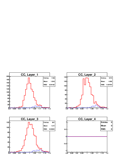
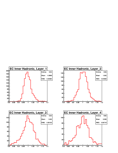
In Fig. 2, as an example, the spread of the calibration constants is plotted for the first hadronic layers of the detector separated into two regions: central calorimeter and EC inner hadronic calorimeter. The calibration constants are mainly in the range of 0.90-1.15 and the root mean squares are at the order of 0.05. Calibration constants are slightly smaller for the central region compared to the EC and for the first hadronic layer compared to the other hadronic layers. The plots of the spread of constants have tails resulting from outliers with higher constants. For the central calorimeter this is mainly due to a single module, whose contribution is plotted separately with dotted lines. In the EC inner hadronic part this outliers are from the region of higher $\eta$’s with the lack of statistics. In these regions only a calibration on tower level is aimed anyway.

The error estimation was done with a MC method: we generate toy simulations of the data with known miscalibrations and compare to the fitted calibration constants of our calibration procedure. The central calorimeter is now calibrated with the precision of the order of 1%, for the high $\eta$-regions it is a few per cent.

Figure 3: $\phi$-intercalibration constants for the first hadronic layer at three different $\eta$-rings at $\eta$ -0.3, -1.6 and -2.4 respectively. The 64 constants corespond to the 64 calorimeter segments in $\phi$-direction.

In general the energy response of the modules is less uniform than it was in Run I. The dominant reason for this is the short integration time in Run II. This amplifies the effect of the finite precision of the calorimeter modules. The electron drift time across the 2.3 mm LAr gap is at the order of 450 ns. While in Run I the integration time was essentially “infinite” on the time scale of this drift time, with the shorter Run II integration time we cut into the signal. The $\phi$-intercalibration accounts for these charge collection effects.

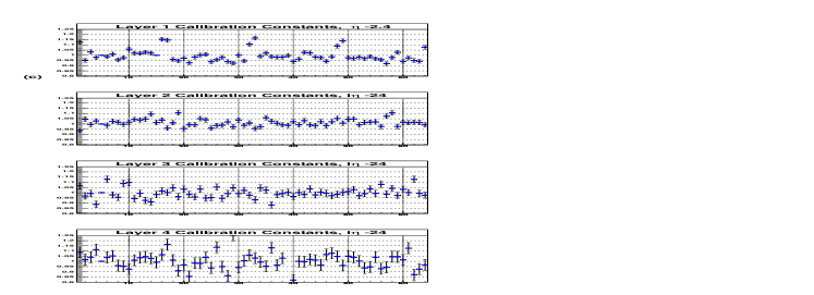
This is illustrated in three examples, where three extreme cases have been choosen. One is a whole module out of the 16 modules in the central calorimeter which has a low response, thus had to be boosted up. As an example we present Fig. 3(a), the calibration constants at $\eta$ of -0.3, but the same pattern is visible in the whole fine hadronic central calorimeter. The spread of calibration constants due to this module is plotted in Fig.2, (dashed line).

In addition, the effect at the edges of this module is stronger and such cells need to be boosted more than at the center of the module. This kind of charge collection effects do not only concern this particular module, they are also visible throughout the hadronic calorimeter. At a closer look to Fig. 3(a), a similar pattern can be recognized for all the modules included in the discussed plot. The same inefficient charge collection is clearly visible in some cells of the end cap calorimeter which are at the boundaries of this calorimeter section. The effects are strongly enhanced by the additional calorimeter borders. An example is plotted in Fig. 3(b) for the $\eta$-ring at -1.6.

The inner hadronic calorimeter was built on one module, thus charge collection effects in the inner hadronic part are of different kind compared to the central part. The inner hadronic modules and absorption layers have been mounted together from half-circles. These modules and absorption layers are oriented within $\pm 90^{\rm o}$ with respect to each other to obtain a structure without any gaps. Charge collection effects due to these rotated semi-circles are visible in the calibration constants. An example is plotted in Fig. 3(c) for the $\eta$-ring at -2.4. Four groups consisting of two constants need to be boosted up due to charge collection effects.

4 $\eta$-intercalibration of the DØ HCAL

The next step in our calibration procedure is the $\eta$-intercalibration, where we determine overall calibration factors for each $\eta$-ring. These will be 64 constants for $-3.2<\eta<3.2$ on top of the $\phi$-intercalibration constants. At this stage the EM layers of the calorimeter are already calibrated and the hadronic cells are equalized in $\phi$. Our aim at the $\eta$-intercalibration is to determine a relative weight between the EM and the hadronic calorimeter which yields the best jet energy resolution. The necessary consequence of this procedure is well known Wigmans:2000vf , the jet response will be non-linear. This is due to the fact that the sampling fraction decreases considerably as the shower develops, because the calorimeter response is smaller for the soft $\gamma$ component in the tail of the shower than for mips. The fraction of energy deposited in the hadronic part of the calorimeter will rise with the energy. The shower starts later and the sampling fraction will rise in this section for the above reasoning. Since a high sampling fraction gives less fluctuations, the hadronic part of the calorimeter demands a higher weight for the best energy resolution. Consequently there are no single optimal constants for all energies. The default constants have been chosen to be optimal for jet of 45 GeV which satisfies the vast majority of physics program at the DØ detector.

Figure 4: $\eta$-intercalibration constants for three different mean jet $p_{T}$ values of 45.2 GeV, 92.3 GeV and 154.6 GeV respectively. Constants are on top of the older ones which roughly reproduced the right sampling fractions.

This discussed non-linearity does not imply that only a certain jet energy is measured correctly. With the presence of the amount of dead material in front of the calorimeter it is anyway non-linear regardless of the weights. The non-linear calorimeter response to jets is corrected with an energy-dependent Jet Energy Scale jiri .

For the $\eta$-intercalibration we used a sample of QCD dijet events where the total missing $p_{T}$-fraction of the events was minimized by weighting the hadronic calorimeter cells within the jets. Only well reconstructed back-to-back two jet events have been selected and an average jet $p_{T}$ well above the trigger threshold was required.

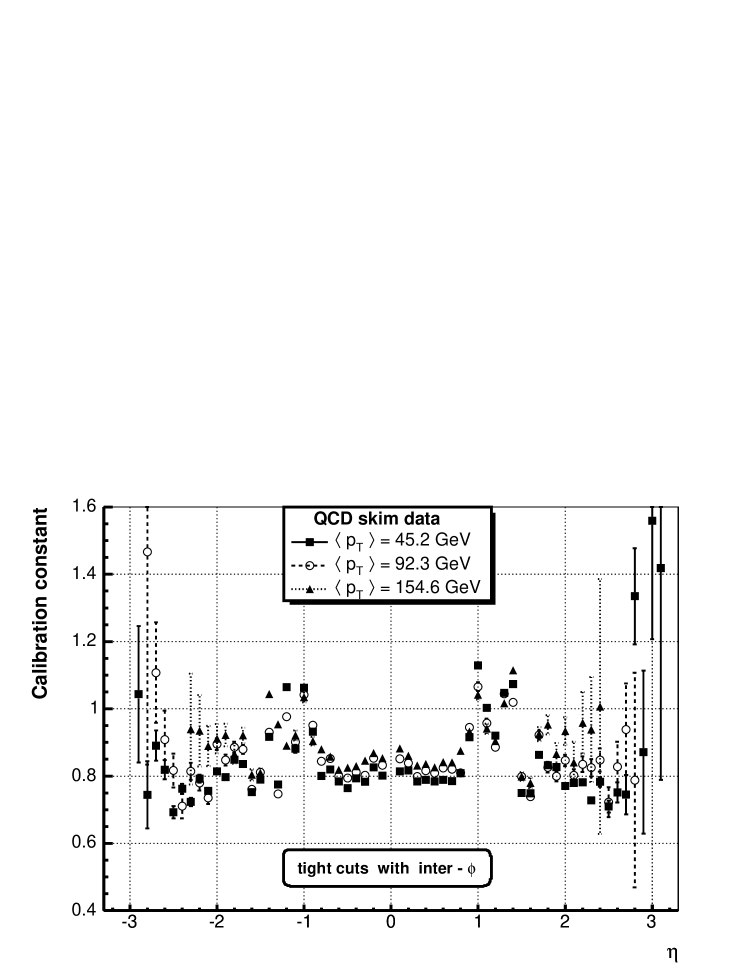
Results of the $\eta$-intercalibration are plotted in Fig.4 for three different mean jet $p_{T}$’s. As discussed, calibration constants rise with the jet $p_{T}$, however there was no appreciable dependence on the jet cone size. These are constants that are on top of the older ones which roughly reproduced the right sampling fractions. There is a discontinuity visible in the constants which is due to the fact that there are no EM cells for $1.2<|\eta|<1.4$. The large error bars at the high $|\eta|$ regions is due to a limited statistics. The correction factor for the regions of $2.0<|\eta|<2.7$ are however stable, thus we choose to extrapolate the mean values of this range to higher $\eta$-values rather than to use the constants with the large errors.

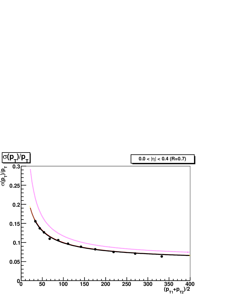
After the full hadronic calorimeter calibration the jet $p_{T}$-resolution were re-determined using dijets and the same 1 fb^-1 sample to account for the improvements due to the hadronic calibration and Jet Energy Scale. The result is plotted in Fig.5 for the $\eta$-range of $0.0<|\eta|<0.4$. The dotted line is the earliest Run II result and the solid line is with the fully calibrated 1 fb^-1 data set. The hadronic calibration lead to significant improvements in the central region (ca. 15% improvement at the energy range of Higgs and top decays).

Figure 5: Jet $p_{T}$-resolution in dijet events from the earliest Run II result (dotted line) and with the fully calibrated 1 fb^-1 data set (solid line) in the $\eta$-range of $0.0<|\eta|<0.4$.

References

- (1) S. Abachi et al. [D0 Collaboration], “The D0 Detector,” Nucl. Instrum. Meth. A 338, 185 (1994).
- (2) V. M. Abazov et al. [D0 Collaboration], “The upgraded D0 detector,” arXiv:physics/0507191, FERMILAB-PUB-05-341-E.
- (3) R. Wigmans, “Calorimetry: Energy measurement in particle physics,” Oxford, UK: Clarendon (2000) 726 p.
- (4) J. Kvita, “Jet Energy Scale determination at DØ,” These proceedings.