Ionization Cooling in all Phase Space Planes with Various Absorber Shapes, Including Parallel-Faced Absorbers

Abstract

Ionization cooling in a straight beamline reduces the transverse emittance of a beam, and has little effect on the longitudinal emittance (generally, in fact, it increases the longitudinal emittance). Once the beamline bends, the introduction of dispersion creates a coupling between the transverse and longitudinal planes. If this coupling is handled properly, one can achieve cooling in all three phase space planes. This is usually done by placing a wedge-shaped absorber in a region where there is dispersion. I will demonstrate using an eigenvalue analysis that there are other configurations of dispersion and absorber shape that will achieve ionization cooling in all phase space planes. In particular, I will show that a one can even achieve cooling in all phase planes with a parallel-faced absorber in a dispersion-free region. I will use perturbation theory to approximate the change in the cooling rates due to longitudinal-transverse coupling. I will then describe how the cooling of longitudinal oscillations can be understood via the projection of the “longitudinal” eigenmodes into the transverse plane.

url]http://pubweb.bnl.gov/people/jsberg/

1 Introduction

Ionization cooling is a method for the rapid reduction of the emittance of a beam by passing the beam through material (hereafter called an “absorber”) [1, 2, 3, 4]. Its primary application has been to muon beams for a neutrino factory or muon collider, but it has been contemplated for other applications as well [5, 6, 7].

In a straight beamline, ionization cooling reduces only the transverse emittance of a beam, generally having little effect on the longitudinal emittance (in fact, generally making it somewhat worse). It reduces the transverse emittance because the total momentum, including the transverse, is reduced when when the beam passes through material, but when the momentum is restored by an RF cavity, the transverse momentum is left unchanged, and thus reduced from its value before the absorber. It is desirable, especially for a muon collider, to reduce the longitudinal emittance as well.

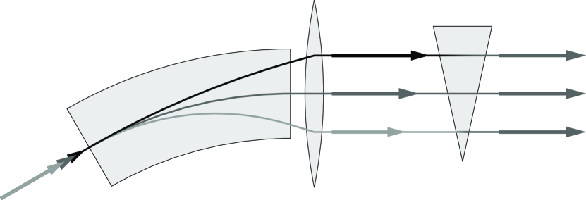
Figure 1: Dispersion generated by a bending magnet (left) means that particles with different energies have different positions. The wedge-shaped absorber (right) then reduces the energies of higher energy particles more than it reduces the energies of lower energy particles.

There is a well-known method for accomplishing this, often referred to as “emittance exchange” [4, 8, 9]. This is generally accomplished by using a wedge-shaped absorber in a region with non-zero dispersion, as shown in Fig. 1. Particles with higher energy will pass through more material than particles with lower energy as a result of the dispersion. Thus, the energy spread in the beam will be reduced. There is a cost to this, however. Imagine that all the energy spread were removed by this. Then there would be no way of removing the spread in transverse position that was introduced by the dispersion. Thus, reduction in longitudinal emittance comes at a cost: the horizontal emittance is increased. If done properly, the cooling accomplished transversely by an absorber can be shared between the longitudinal and transverse planes, giving emittance reduction in all phase space planes.

This paper will demonstrate that achieving cooling in the longitudinal plane can be accomplished by a more general class of methods than just having dispersion in transverse position at a wedge-shaped absorber. It will demonstrate that cooling in all planes happens when there is an appropriate coupling between the longitudinal and transverse planes. The paper will explore multiple ways of generating that coupling and compare their effectiveness.

I will first describe a simplified lattice that will be used in this paper. I will then ascertain whether the lattice is cooling in all phase space planes by examining the eigenvalues for the linear matrix representing that lattice. I will compute the eigenvalues approximately using perturbation theory, where the small parameter in the expansion is the degree of coupling between the longitudinal and transverse planes. I will study coupling that is generated by dispersion and an appropriately shaped absorber, and coupling generated by dispersion in the RF cavity. I will then look at the eigenvalues for cases when the perturbation expansion might not be accurate. Finally, I will develop a more physically intuitive understanding of how transverse cooling can reduce the longitudinal emittance by examining the motion in the coupled system using the eigenvectors of the matrix that represents the lattice, which will give a picture of the coupled motion when it is projected into the longitudinal and transverse planes.

This paper does not address other issues of cooling lattice design, in particular the final equilibrium emittance which results because of multiple scattering and energy straggling. The paper is intended only to present a wider range of ideas on how cooling can be accomplished in all phase space planes, not to present a full generalized theory of ionization cooling or a working cooling lattice design.

2 Lattice

The cooling lattice will consist of a sequence of identical cells with four sections:

1. An absorber, which reduces the energy of the particles

2. An RF cavity, which restores the energy lost in the absorber and provides longitudinal focusing

3. A group of magnets transporting the beam from the absorber to the next RF cavity

4. A group of magnets transporting the beam from the cavity to the next absorber

The details of what is in the “group of magnets” will not be important for this discussion.

There is a planar reference curve which defines the coordinate system that we are using. The vertical coordinate $y$ is perpendicular to the plane in which the curve lies. The horizontal coordinate $x$ is perpendicular to the vertical and to the tangent to the curve, and stays on the same side of the curve. The arc length along the curve, $s$, is the independent variable for the equations of motion. For the examples in this paper, the vertical magnetic field at the reference curve $B_{0}(s)$ will be such that a particle with a reference energy $E_{\text{r}}(s)$ which starts out on the curve and moving tangent to the curve continues to do so. This particle will be referred to as the reference particle. Note that the reference energy depends on the position in the lattice, due to the absorber and the RF cavity.

The magnetic field will be midplane symmetric, meaning that the vertical field is symmetric under $y\to-y$, and the other magnetic fields are antisymmetric under $y\to-y$. There are two consequences of this. The first is that this is not a solenoid focused lattice, which is typical for an ionization cooling lattice, but a quadrupole-focused lattice. The second is that the vertical motion is, to lowest order, decoupled from the horizontal and longitudinal motions. This second reason is the fundamental purpose in choosing a midplane symmetric lattice. The qualitative results found here will continue to hold for a solenoid-focused lattice.

The reference particle will lose an energy $\Delta E$ in the absorber and will gain back that same amount energy in the RF cavity. The energies in the magnets between these elements will be $E_{\pm}=E_{0}\pm\Delta E/2$, the corresponding total momenta are $p_{\pm}=\sqrt{E_{\pm}^{2}/c^{2}-(mc)^{2}}$, and $p_{0}=\sqrt{E_{0}^{2}/c^{2}-(mc)^{2}}$. In these expressions $m$ is the particle mass and $c$ is the speed of light.

2.1 Matrices for Lattice Sections

I want to determine whether for small deviations from the particle with coordinates zero, the amplitude of oscillations is growing or reducing. Thus, this paper will only keep results to first order in these deviations, and will use matrices to represent how these deviations change while propagating through the lattice. The lattice is a sequence of identical cells, and the eigenvalues for the matrix for an entire cell will determine the characteristics of the motion.

I will denote the absorber location by a subscript “a,” and the cavity location by a subscript “c.” The matrix describing the motion through the magnets from the absorber to the cavity is $\mathcal{M}_{\text{ca}}$, and the matrix from the cavity to the absorber is $\mathcal{M}_{\text{ac}}$. I will assume a kind of reflection symmetry at the absorber and cavity such that these matrices can be written as

$$\mathcal{M}_{\text{ac}} =\mathcal{D}_{\text{a}}\mathcal{B}_{\text{a}}\mathcal{R}(\mu_{-},R_{56}^{-})\mathcal{B}_{\text{c}}^{-1}\mathcal{D}_{\text{c}}^{-1}$$ (1)

$$\mathcal{M}_{\text{ca}} =\mathcal{D}_{\text{c}}\mathcal{B}_{\text{c}}\mathcal{R}(\mu_{+},R_{56}^{+})\mathcal{B}_{\text{a}}^{-1}\mathcal{D}_{\text{a}}^{-1},$$ (2)

where

$$\mathcal{B}_{i} =\begin{bmatrix}b_{i}^{1/2}&0&0&0\\ 0&b_{i}^{-1/2}&0&0\\ 0&0&1&0\\ 0&0&0&1\end{bmatrix}$$ (3)

$$\mathcal{R}(\mu,R_{56}) =\begin{bmatrix}\cos\mu&\sin\mu&0&0\\ -\sin\mu&\cos\mu&0&0\\ 0&0&1&R_{56}\\ 0&0&0&1\end{bmatrix}$$ (4)

$$\mathcal{D}_{i} =\begin{bmatrix}1&0&0&d_{i}^{x}\\ 0&1&0&d_{i}^{p}\\ d_{i}^{p}&-d_{i}^{x}&1&0\\ 0&0&0&1\end{bmatrix}.$$ (5)

These quantities are related to the usual accelerator quantities by $b_{i}=\beta_{x}(s_{i})/p_{\text{r}}(s_{i})$, $d_{i}^{x}=D(s_{i})/[\beta_{\text{r}}(s_{i})p_{\text{r}}(s_{i})c]$, and $d_{i}^{p}=D^{\prime}(s_{i})/[\beta_{\text{r}}(s_{i})c]$, where $p_{\text{r}}(s)=\sqrt{E^{2}_{\text{r}}(s)/c^{2}-(mc)^{2}}$, $\beta_{\text{r}}(s)=p_{\text{r}}(s)c/E_{\text{r}}(s)$, $\beta_{x}(s)$ is the Courant-Snyder beta function, and $D(s)$ is the dispersion. Note that since $p_{\text{r}}(s_{\text{a}})=p_{\pm}$ depending on which side of the absorber one is on, the beta functions on each side of the absorber are actually slightly different. The same type of difference exists for the cavity and the dispersion.

Assuming that the only effect of the RF cavity and absorber is to shift the energy of all particles by $\pm\Delta E$, the matrix for the full cell from the absorber back to the next absorber is

$$\mathcal{D}_{\text{a}}\mathcal{B}_{\text{a}}\mathcal{R}(\mu_{-}+\mu_{+},R_{56}^{-}+R_{56}^{+})\mathcal{B}_{\text{a}}^{-1}\mathcal{D}_{\text{a}}^{-1}$$ (6)

Thus, the transverse phase advance per cell is $\mu_{-}+\mu_{+}$, and $R_{56}^{-}+R_{56}^{+}$ is approximately $\eta_{c}TE/(pc)^{2}$, where $\eta_{c}$ is the frequency slip factor, and $T$ is the time for the reference particle to go through one cell. The momentum $p$ and energy $E$ are intentionally left ambiguous: $\eta_{c}$ is only defined for a fixed energy.

The RF cavity is described by a matrix

$$\mathcal{V}=\begin{bmatrix}1&0&0&0\\ 0&1&0&0\\ 0&0&1&0\\ 0&0&\omega V\cos\phi&1\end{bmatrix},$$ (7)

where $V$ is the maximum energy gain in the cavity, the RF phase is $\phi$, where $\phi=0$ is the phase for zero energy gain, and $\omega$ is $2\pi$ times the RF frequency.

The absorber reduces the energy of the particles, maintaining their direction. The horizontal position will thus be the same as it would be if the absorber were a drift. The time to traverse the absorber is well approximated by assuming that the momentum is $p_{+}$ to the center of the absorber, then $p_{-}$ thereafter. Thus, it is a good approximation to treat the absorber as a thin element, with surrounding drifts absorbed into $\mathcal{M}_{\text{ac}}$ and $\mathcal{M}_{\text{ca}}$.

Since the particle direction is maintained, the transverse momentum will be reduced in the absorber by the same factor that the total momentum is reduced, $\kappa_{x}=p_{-}/p_{+}$. Particles whose energy differs from the reference energy will receive a slightly different energy loss than the reference particle, since the energy loss per unit length in the absorber, $dE/dx$, depends on energy. To linear order, the energy loss of a particle with energy $E$ just before the absorber is

$$\Delta E+\Delta E\left(\dfrac{dE}{dx}\right)^{-1}\dfrac{d}{dE}\left(\dfrac{dE}{dx}\right)(E-E_{+})\\ \mbox{}=\Delta E+(1-\kappa_{z})(E-E_{+})$$ (8)

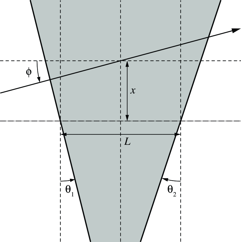
Figure 2: Geometry of the absorber. $\sin\phi=p_{x}/p_{+}$, where $p_{x}$ is the horizontal momentum before the absorber.

Furthermore, if the faces of the absorber are not perpendicular to the reference orbit, there may be an energy loss which depends on the horizontal position or angle (again, I’m ignoring the vertical motion). Using the geometry from Fig. 2, the change in the energy is $a_{+}x+a_{-}Lp_{x}/(2p_{+})$ [10], where

$$a_{\pm}=-\dfrac{dE}{dx}(\tan\theta_{2}\pm\tan\theta_{1}).$$ (9)

These define the matrix for the absorber, which I will denote $\mathcal{A}$:

$$\mathcal{A}=\begin{bmatrix}1&0&0&0\\ 0&\kappa_{x}&0&0\\ 0&0&1&0\\ a_{+}&a_{-}L/(2p_{+})&0&\kappa_{z}\end{bmatrix}.$$ (10)

3 Eigenvalue Analysis

The transfer matrix for the full lattice,including the absorbers and the RF cavities, is

$$\mathcal{A}\mathcal{M}_{\text{ac}}\mathcal{V}\mathcal{M}_{\text{ca}}.$$ (11)

I will be analyzing the eigenvalues of this matrix to determine if I am achieving cooling in both planes. First of all, it is clear that the product of the eigenvalues is $\kappa_{x}\kappa_{z}$, and that the eigenvalues will come in complex conjugate pairs.

Begin with a basic lattice, with no dispersion, and with the absorber face angle $\theta_{1}=\theta_{2}=0$. The characteristic polynomial for the matrix for the cell is

$$(\lambda^{2}-\lambda(1+\kappa_{z}+(R_{56}^{-}+\kappa_{z}R_{56}^{+})\omega V\cos\phi)+\kappa_{z})\\ (\lambda^{2}-\lambda(1+\kappa_{x})\cos(\mu_{+}+\mu_{-})+\kappa_{x}).$$ (12)

The roots of the characteristic polynomial are the eigenvalues.

From this polynomial, we can see that the eigenvalues will be of the form

$$\sqrt{\kappa_{x}}e^{\pm i\mu_{x}} \sqrt{\kappa_{z}}e^{\pm i\mu_{z}}.$$ (13)

It turns out that the eigenvalues remain the same if $d_{\text{a}}^{x}$ and $d_{\text{a}}^{p}$ are nonzero, as long as one minor correction is applied: in $\mathcal{M}_{\text{ac}}$, $d_{\text{a}}^{x}$ should be replaced with $d_{\text{a}}^{x}\sqrt{\kappa_{x}}$, and in $\mathcal{M}_{\text{ca}}$, $d_{\text{a}}^{x}$ should be replaced with $d_{\text{a}}^{x}/\sqrt{\kappa_{x}}$.

Thus, $\sqrt{\kappa_{x}}$ is the magnitude of the transverse eigenvalue, and $\sqrt{\kappa_{z}}$ is the magnitude of the longitudinal eigenvalue. Clearly $\kappa_{x}<1$; unfortunately, in most cases of interest for cooling, $\kappa_{z}>1$. However, the product $\kappa_{x}\kappa_{z}<1$. $\kappa_{z}>1$ because for low energies, $(d/dE)(dE/dx)<0$. While $(d/dE)(dE/dx)$ becomes positive for higher energies, the relative energy loss for a given absorber is less at higher energies, making $\kappa_{x}$ closer to 1, and the product $\kappa_{x}\kappa_{z}$ closer to 1.

Since the product $\kappa_{x}\kappa_{z}<1$, if one could generate coupling between the horizontal and vertical motion, it would be possible to reduce the magnitude of the “longitudinal” eigenvalues (they begin to lose their identity with coupling), at the cost of raising the magnitude of the “transverse” eigenvalues. One could do so in a way that made the magnitudes of both sets of eigenvalues less than 1, and thus gave cooling in all phase space planes.

If the characteristic polynomial for a matrix is Eq. (12) plus some additional polynomial $f(\lambda)$, then one can compute the change in the eigenvalues to lowest order. The lowest-order change in the magnitude of $\lambda_{x}=\sqrt{\kappa_{x}}e^{i\mu_{x}}$ is

$$-\dfrac{\csc\mu_{x}}{2\sqrt{\kappa_{x}}}\operatorname{Im}\left\{\dfrac{e^{-i\mu_{x}}f(\lambda_{x})}{(\lambda_{x}-\lambda_{z})(\lambda_{x}-\lambda^{*}_{z})}\right\}$$ (14)

and the lowest-order change in the magnitude of $\lambda_{z}=\sqrt{\kappa_{z}}e^{i\mu_{z}}$ is

$$-\dfrac{\csc\mu_{z}}{2\sqrt{\kappa_{z}}}\operatorname{Im}\left\{\dfrac{e^{-i\mu_{z}}f(\lambda_{z})}{(\lambda_{z}-\lambda_{x})(\lambda_{z}-\lambda^{*}_{x})}\right\}.$$ (15)

Since a change in the magnitude of $\lambda_{z}$ leads to a corresponding change in the magnitude of $\lambda_{x}$, one only need examine the change in one eigenvalue.

Note that when $\lambda_{x}$ is close to $\lambda_{z}$ or $\lambda_{z}^{*}$, there will be a large change in the eigenvalues. This corresponds to a linear coupling resonance between the longitudinal and horizontal. For our perturbation analysis, we will assume that we are sufficiently far from that resonance condition, but this will be of interest later in the paper nonetheless.

Since $f$ is the difference between the characteristic polynomial for the full system and Eq. (12), we know something more about its properties. First of all, it is a third order polynomial, since all characteristic polynomials of a $4\times 4$ matrix are fourth order polynomials with leading order term $\lambda^{4}$. Secondly, the constant term in the characteristic polynomial is the determinant, and the determinant of the matrix is $\kappa_{x}\kappa_{z}$ in all cases. Thus, $f$ will have no constant term. We can thus write $f(\lambda)$ as $f_{3}\lambda^{3}+f_{2}\lambda^{2}+f_{1}\lambda$.

I will examine the change in the magnitude of $\lambda_{z}$. Using the polynomial expression for $f(\lambda)$, it is

$$\dfrac{\begin{aligned} &2\sqrt{\kappa_{x}\kappa_{z}}(\kappa_{z}f_{3}-f_{1})\cos\mu_{x}\\ &\mspace{2.0mu}\mbox{}-2\kappa_{z}(\kappa_{x}f_{3}-f_{1})\cos\mu_{z}+\sqrt{\kappa_{z}}(\kappa_{z}-\kappa_{x})f_{2}\end{aligned}}{\begin{aligned} &2[\kappa_{z}+\kappa_{x}-2\sqrt{\kappa_{x}\kappa_{z}}\cos(\mu_{x}-\mu_{z})]\\ &\mspace{80.0mu}[\kappa_{z}+\kappa_{x}-2\sqrt{\kappa_{x}\kappa_{z}}\cos(\mu_{x}+\mu_{z})]\end{aligned}}.$$ (16)

There are two methods for generating coupling between the phase space planes. The most common method is to create an absorber with nonzero values for the angles $\theta_{1}$ and $\theta_{2}$ (in most cases with $\theta_{1}=\theta_{2}$, thus referred to as a “wedge”). Another method is to generate the coupling by having dispersion in the RF cavity, which does not require any change in the shape of the absorber.

3.1 Rotated Absorber Faces

The additional terms in the characteristic polynomial when $\theta_{0}$ or $\theta_{1}$ are nonzero but the dispersion at the cavity is zero are

$$\dfrac{a_{+}d^{x}_{\text{a}}}{\sqrt{\kappa_{x}}}[\lambda^{3}(\cos\mu_{x0}-\kappa_{x}s_{+})\\ \mbox{}+\lambda^{2}\cos\mu_{x0}(\kappa_{x}^{2}s_{+}-s_{-})\\ \mbox{}+\lambda\kappa_{x}(s_{-}-\kappa_{x}\cos\mu_{x0})]\\ \mbox{}+a_{+}d^{p}_{\text{a}}b_{\text{a}}\sin\mu_{x0}[\lambda^{3}-\lambda^{2}(\kappa_{x}s_{+}+s_{-})+\lambda\kappa_{x}]\\ \mbox{}-\dfrac{a_{-}Ld_{\text{a}}^{x}}{2p_{+}\sqrt{\kappa_{x}}b_{\text{a}}}\sin\mu_{x0}[\lambda^{3}-\lambda^{2}(\kappa_{x}s_{+}+s_{-})+\lambda\kappa_{x}]\\ \mbox{}+\dfrac{a_{-}Ld^{p}_{\text{a}}}{2p_{+}}[\lambda^{3}(\cos\mu_{x0}-s_{+})\\ \mbox{}+\lambda^{2}\cos\mu_{x0}(s_{+}-s_{-})\\ \mbox{}+\lambda(s_{-}-\cos\mu_{x0})],$$ (17)

where $\mu_{x0}=\mu_{+}+\mu_{-}$ and $s_{\pm}=1+R_{56}^{\pm}\omega V\cos\phi$. Note that from Eq. (12), $\kappa_{z}s_{+}+s_{-}=2\sqrt{\kappa_{z}}\cos\mu_{z}$. The numerator of Eq. (16) for this case is $\sqrt{\kappa_{z}}$ times

$$\dfrac{a_{+}d_{\text{a}}^{x}}{\sqrt{\kappa_{x}}}[s_{-}+\kappa_{x}s_{+}-(1+\kappa_{x})\cos\mu_{x0}]\\ [\kappa_{x}(s_{-}+s_{+}\kappa_{z})-(\kappa_{x}^{2}+\kappa_{z})\cos\mu_{x0}]\\ \mbox{}-a_{+}d_{\text{a}}^{p}b_{\text{a}}(\kappa_{z}-\kappa_{x})\sin\mu_{x0}\\ [s_{-}+\kappa_{x}s_{+}-(1+\kappa_{x})\cos\mu_{x0}]\\ \mbox{}+\dfrac{a_{-}Ld_{\text{a}}^{x}}{2p_{+}\sqrt{\kappa_{x}}b_{\text{a}}}(\kappa_{z}-\kappa_{x})\sin\mu_{x0}\\ [s_{-}+\kappa_{x}s_{+}-(1+\kappa_{x})\cos\mu_{x0}]\\ \mbox{}+\dfrac{a_{-}Ld_{\text{a}}^{p}}{2p_{+}}[s_{-}+\kappa_{x}s_{+}-(1+\kappa_{x})\cos\mu_{x0}]\\ [s_{-}+s_{+}\kappa_{z}-(1+\kappa_{z})\cos\mu_{x0}].$$ (18)

Since $\kappa_{x}\approx\kappa_{z}\approx 1$ in most cases, the quantity $\kappa_{z}-\kappa_{x}$ can be treated as small. Thus, the second and third terms in Eq. (18) can be neglected, as long as one is far from the linear synchro-betatron resonance. Equation (18) indicates that if one has a dispersion in position but not momentum at the absorber, the absorber should have $\theta_{1}=\theta_{2}$ (i.e., a wedge shape), and $\theta_{1}$ positive if the dispersion is positive. This is the usual method of “emittance exchange.”

If, on the other hand, there is no dispersion in position but there is dispersion in horizontal momentum, one should instead use a rotated slab (i.e., $\theta_{1}=-\theta_{2}$). Particles with larger momentum will have an angle in one direction; if the absorber is rotated so there is more material along that direction, there will be a greater energy loss for those particles.

One might ask whether it is easier to construct a lattice that makes the first term large than it is to construct a lattice that makes the fourth term large. In fact, either term can be made large, and which one is used depends on the desired properties of the lattice. Take, for instance, the RFOFO cooling ring described in [11]. $(dE/dx)d_{\text{a}}^{x}$ for that lattice is about 0.027. If one finds the largest value of the momentum dispersion, then $(dE/dx)Ld_{\text{a}}^{p}/(2p_{+})$ is around 0.002. While it may seem that the former is significantly larger than the latter, the fact is that the lattice was designed with a ring shape, which tends to generate position dispersion rather than momentum dispersion. One can construct lattices where $(dE/dx)Ld_{\text{a}}^{p}/(2p_{+})$ is larger, especially when the beta function at the absorber is small, by having one half of the lattice cell bending in one direction and and the other half bending in the reverse direction.

3.2 Dispersion in the RF Cavity

If instead, $\theta_{0}=\theta_{1}=0$, but we have dispersion at the cavity, there is still coupling between the longitudinal and transverse planes, in this case generated by the dispersion at the RF cavity. The additional terms in the characteristic polynomial are

$$\dfrac{\omega V\cos\phi}{2b_{\text{c}}}\lambda(\lambda-1)(\lambda-\kappa_{z})\\ \{[(d_{\text{c}}^{x})^{2}+b_{\text{c}}^{2}(d_{\text{c}}^{p})^{2}](\kappa_{x}+1)\sin(\mu_{+}+\mu_{-})\\ \mbox{}-[(d_{\text{c}}^{x})^{2}-b_{\text{c}}^{2}(d_{\text{c}}^{p})^{2}](\kappa_{x}-1)\sin(\mu_{+}-\mu_{-})\\ \mbox{}-2b_{\text{c}}d_{\text{c}}^{x}d_{\text{c}}^{p}(\kappa_{x}-1)\cos(\mu_{+}-\mu_{-})\}$$ (19)

The numerator of Eq. (16) is then

$$\dfrac{\omega V\cos\phi}{2b_{\text{c}}}(\kappa_{z}-\kappa_{x})[2\kappa_{z}\cos\mu_{z}-\sqrt{\kappa_{z}}(1+\kappa_{z})]\\ \{[(d_{\text{c}}^{x})^{2}+b_{\text{c}}^{2}(d_{\text{c}}^{p})^{2}](\kappa_{x}+1)\sin(\mu_{+}+\mu_{-})\\ \mbox{}-[(d_{\text{c}}^{x})^{2}-b_{\text{c}}^{2}(d_{\text{c}}^{p})^{2}](\kappa_{x}-1)\sin(\mu_{+}-\mu_{-})\\ \mbox{}-2b_{\text{c}}d_{\text{c}}^{x}d_{\text{c}}^{p}(\kappa_{x}-1)\cos(\mu_{+}-\mu_{-})\}$$ (20)

For the RFOFO ring in [11], the quantity

$$\dfrac{\omega V\cos\phi}{2b_{\text{c}}}(d_{\text{c}})^{2}$$ (21)

is around $1.7\times 10^{-3}$. The product of the next two factors in Eq. (20) is around $-0.02$. Thus, compared to an absorber with substantial rotations in its faces, the strength of the coupling generated by dispersion in the RF cavities is relatively weak. The RFOFO ring was not necessarily designed for maximizing coupling in this way, but it is unlikely to be possible to increase the dispersion sufficiently while keeping a reasonably small beta function in the lattice. One may be able to increase the RF voltage somewhat, but certainly not enough to change the overall result.

3.3 Running Closer to Resonance

The perturbation theory analysis assumed that one was far from the point where any two of the eigenvalues of the matrix are close to each other. If they do become close, then the estimates above are not valid, and the eigenvalues should be computed directly.

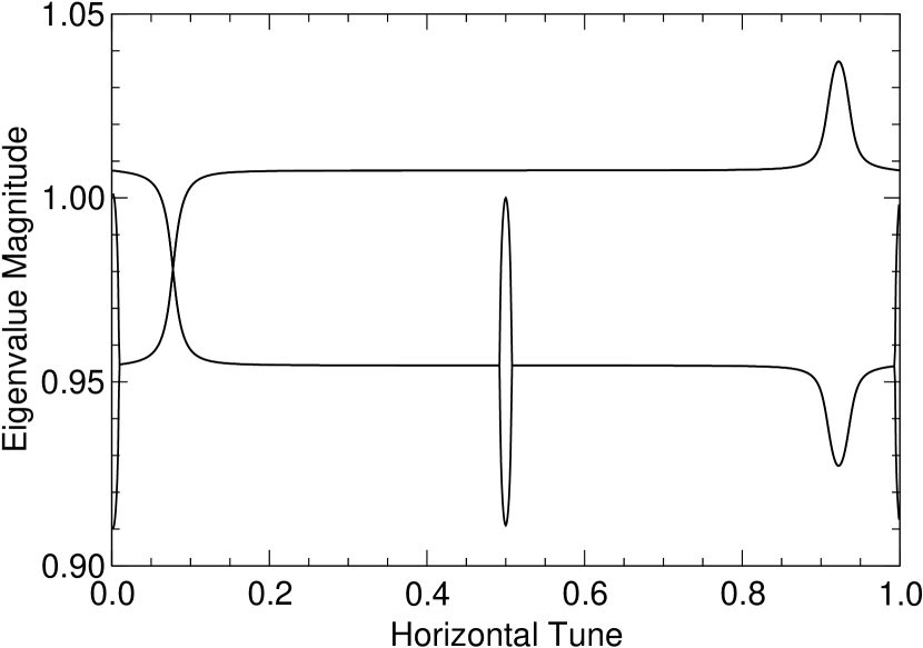
Figure 3: Magnitude of matrix eigenvalues as a function of $(\mu_{+}+\mu_{-})/(2\pi)$ for a lattice with dispersion at the RF cavities and an absorber with $\theta_{1}=\theta_{2}=0$.

Begin with the case where there is dispersion in the RF cavity and $\theta_{0}=\theta_{1}=0$. Figure 3 shows the magnitude of the eigenvalues as a function of $\mu_{+}+\mu_{-}$, where I am taking $\mu_{+}=\mu_{-}$. Note that when $(\mu_{+}+\mu_{-})/(2\pi)\approx 0.08$, which is the synchrotron tune, then the magnitudes of all the eigenvalues become less than 1 [12]. What one is seeing here is the manifestation of a coupling resonance in a non-conservative dynamical system. Note that the same resonance phenomenon at $(\mu_{+}+\mu_{-})/(2\pi)\approx 1-0.08$ results in the longitudinal eigenvalue becoming more unstable: instead of the resonance pulling the eigenvalues together, it pushes them further apart. The signs of these effects are consistent with what one expects from the perturbation calculation in Eq. (20): the sign of $\sin(\mu_{+}+\mu_{-})$ gives the dominant effect for determining whether the magnitude of the longitudinal eigenvalue increases or increases. The loops in Fig. 3 near the tunes of 0 and 0.5 are not important for this discussion: they are simply the linear resonances of the transverse lattice.

This example is furthermore an example of how a difference resonance ($\nu_{x}-\nu_{z}=k$ in this case) tends to lead to often innocuous coupling between planes, whereas a sum resonance ($\nu_{x}+\nu_{z}=k$ in this case) can lead to unbounded growth. The coupling between the planes is in fact an advantage in this case, since one is trying to make the transverse damping affect the longitudinal plane.

Having a low horizontal tune is generally impractical for cooling channels, since that tends to give a larger beta function at the absorber, which results in a larger equilibrium emittance due to multiple scattering [3, 4]. However, one could instead run in the passband with horizontal tunes from 1 to 1.5, which would both create a low beta function and ensure that coupling pulled the magnitudes of the eigenvalues closer to each other. It would also allow for a longer cell, making it possible to increase the synchrotron tune, putting it further from the integer resonance. It may be more difficult to have a large momentum acceptance in such a lattice, however, since the passband from tunes of 1 to 1.5 generally would have a smaller relative momentum acceptance than the lower passbands.

This example is meant more as a proof of principle, demonstrating that one can in principle use any method of longitudinal-transverse coupling to achieve cooling in all degrees of freedom. The method may, however, have practical applications in cases where it is impractical to control the shape of the absorber. One example might be the use of a lithium lens in the final stages of cooling for a muon collider. The method may be more interesting at later stages of a muon collider in any case, since the limited width of the resonance will likely translate into a limited momentum acceptance for such a method, requiring a beam which has already had its longitudinal emittance reduced significantly.

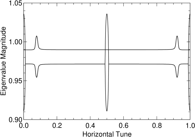
Figure 4: Magnitude of matrix eigenvalues as a function of $(\mu_{+}+\mu_{-})/(2\pi)$ for a lattice with dispersion at a wedge shaped absorber.

It is interesting to compare Fig. 3 with what one would obtain when using a wedge-shaped absorber with dispersion. This is shown in Fig. 4. Note that the eigenvalue magnitudes are closer to each other over the entire range of horizontal tunes (their values without dispersion at the wedges can be deduced from Fig. 3). At both the sum and difference resonances, the magnitudes are pushed further apart. The difference in the behavior near the synchro-betatron resonances between this case and that shown in Fig. 3 is a result of the non-symplectic nature of the coupling that is generated by the wedge with dispersion. Eqs. (16) and (18) do an extremely good job of predicting the behavior in Fig. 4, including the resonant behavior; this is to be expected since the eigenvalues never get too close together, even near the resonance.

4 Physical Explanation

To get some understanding of what is going on physically, one should examine the eigenvectors. The real and imaginary parts of the eigenvectors define an ellipse that the particles move on. Of course, in the case of cooling, the radius of the particles are decreasing (or sometimes increasing), but that piece can be taken out (i.e., the difference of the magnitude of the eigenvalue from 1). To see the ellipse, take the real (or imaginary) part of the eigenvector, multiply the vector by the matrix for the lattice cell, and divide the result by the magnitude of the corresponding eigenvalue. Repeat the process, and one will trace out an ellipse in phase space. Alternatively, if $\vec{v}$ is the eigenvector, then the ellipse is the set of points obtained from

$$\operatorname{Re}\{\vec{v}\}\cos u+\operatorname{Im}\{\vec{v}\}\sin u$$ (22)

by varying $u$ from 0 to $2\pi$.

In the case where there is no coupling, the eigenvectors have components either entirely in the horizontal plane, or entirely in the longitudinal (time-energy) plane. However, once one introduces any type of longitudinal-transverse coupling, all of the eigenvectors will have components in both planes. This is the key to what allows the reduction in transverse momentum spread that the absorber accomplishes to reduce the amplitude of what would otherwise be longitudinal motion. The only effect that actually reduces the beam emittance is the reduction of transverse momentum in the absorber.

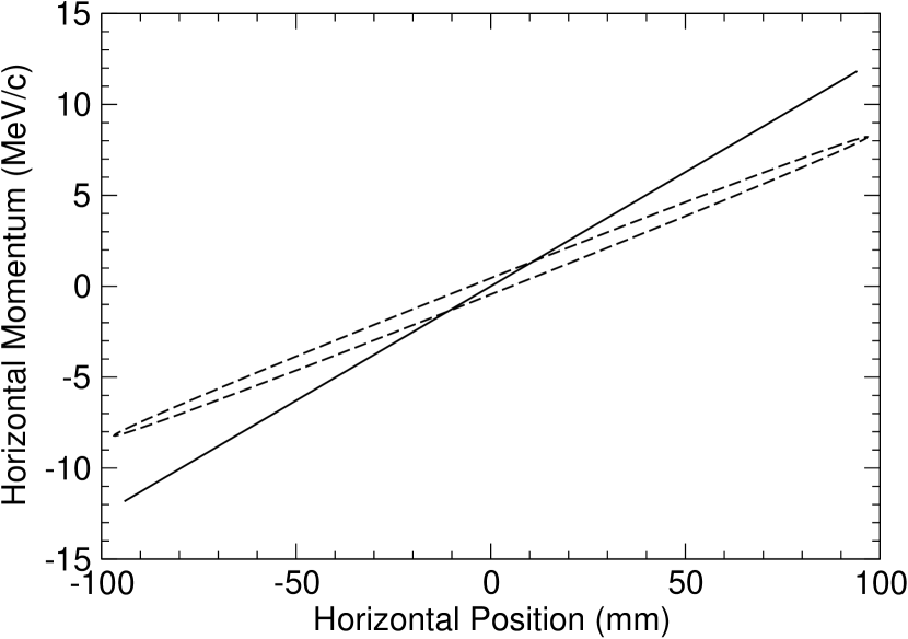
Figure 5: Projection of the longitudinal eigenvector at the absorber into the transverse plane when there is dispersion at the absorber. The solid ellipse (which has no area, so it appears as a line) is for a parallel-faced absorber ($\theta_{1}=\theta_{2}=0$), whereas the dashed ellipse is for a wedge-shaped absorber.

Figure 5 shows the projection of the longitudinal eigenvector (identified by the phase of its corresponding eigenvalue) at the absorber into the transverse plane. The figure shows two cases: one where there is dispersion at the absorber, but the absorber has parallel faces with $\theta_{1}=\theta_{2}=0$, and one where the absorber is wedge shaped, with $\theta_{1}=\theta_{2}>0$. For the parallel-faced case, there is no reduction in the magnitude of the longitudinal eigenvalue, despite the fact that Fig. 5 shows that there is a nonzero projection of the longitudinal eigenvalue onto the horizontal plane (and horizontal momentum in particular). The reason that there is no reduction in the magnitude of the longitudinal eigenvalue is that the ellipse projected into the horizontal plane has no area. The absorber makes positive momenta more negative and negative momenta more positive, reducing the area of an ellipse. But if the ellipse has no area, no reduction can occur. Thus, one needs the projected ellipse to have a nonzero area to see an effect. This is what making the absorber wedge-shaped accomplishes, as can be seen in Fig. 5.

If one changes the horizontal tune to around 0.077, one can see from Fig. 4 that the longitudinal and transverse eigenvalues return almost to their values without coupling. This is reflected in the eigenvectors in that the area of the horizontal projection of the ellipse relative to the area of the longitudinal projection is less than it was for horizontal tunes away from the longitudinal tune (which was shown in Fig. 5).

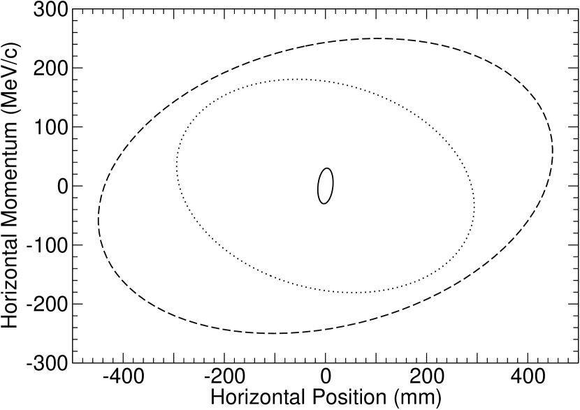
Figure 6: Projection of the longitudinal eigenvector at the absorber into the transverse plane when there is a parallel-faced absorber and dispersion only at the RF cavity. The solid ellipse is for a horizontal tune of 0.75, the dotted ellipse for a horizontal tune of 0.09 (near one coupling resonance), and the dashed ellipse for a horizontal tune of 0.91 (near the other coupling resonance).

Figure 6 shows the ellipses for the case where there is dispersion at the RF cavity and not the absorber (this corresponds to Fig. 3). The ellipses are smaller when one is away from resonance, and larger when one is closer to resonance, reflecting the stronger coupling between the eigenvalues near the resonance, in particular that the magnitude of the longitudinal eigenvalue is reduced (or increased for the higher-tune resonance) there. What the figure does not illustrate is why near the low tune resonance (0.09 for the example in Fig. 6), the magnitude of the longitudinal eigenvalue is reduced, whereas near the high tune resonance, the magnitude of the longitudinal eigenvalue is increased.

To understand this, one must first think about what area means for an ellipse in four-dimensional phase space. Hamilton’s equations of motion can be written as

$$\dfrac{d\vec{z}}{ds}=-J\vec{\nabla}H(\vec{z},s),$$ (23)

where for the example here where only horizontal and longitudinal dimensions are considered,

$$J=\begin{bmatrix}0&1&0&0\\ -1&0&0&0\\ 0&0&0&-1\\ 0&0&1&0\end{bmatrix}.$$ (24)

One can define the area of a four-dimensional ellipse which is described by Eq. (22) to be $\pi$ times

$$(\operatorname{Im}\{\vec{v}\})^{T}J(\operatorname{Re}\{\vec{v}\}).$$ (25)

This gives the expected answer when the ellipse lies entirely in either the horizontal or longitudinal phase space plane, and is thus the obvious extension of the concept. In fact, it is really the sum of the projected areas in the two planes. Furthermore, it is invariant under symplectic transformations of $\vec{v}$, and thus reflects the area-preserving nature of symplectic transformations.

Note that this area, as defined, has a sign. Since the eigenvectors come in complex-conjugate pairs, there are always two areas with the same magnitude and opposite signs generated by the eigenvectors of a matrix, assuming the eigenvectors were not normalized differently. Furthermore, since the area is really a sum of the horizontal area and the longitudinal area, these projected areas individually have signs as well. It turns out that when the longitudinal eigenvalue gets closer in magnitude to the transverse one, the areas have the same sign, whereas when they are pushed away from each other, the areas have opposite signs.

Physically, this is because the sign of the ellipse area is related to the direction which a particle moves around the ellipse in phase space, as can be seen from Eq. (22). There is a “physical” direction that particles move around an ellipse, which is reflected in the signs of the nonzero elements in $J$. Normally, particles with positive horizontal momentum will have an increasing horizontal position; particles with a larger energy will have a shorter time of flight (ignoring momentum compaction). When the signs of the projected areas (horizontal and longitudinal) are identical, the particles are moving in the “physical” direction on both the horizontal and longitudinal ellipses. If, on the other hand, the projected areas have opposite signs, then longitudinal motion in the “physical” direction will appear to have “unphysical” motion in the horizontal plane. Thus, in particular, the reduction in horizontal momentum that the absorber accomplishes will not be translated physically into the area reduction that one hopes for, since the change in horizontal position goes the wrong way. The result is the eigenvalue magnitudes getting further apart, as seen on the right hand side of Fig. 3.

5 Conclusion

I have shown that one can obtain ionization cooling in all phase space planes through two different methods: by generating dispersion at the absorber and shaping the absorber appropriately (this is the usual method), and by using the longitudinal-transverse coupling resonance with a parallel-faced absorber. I have approximated the effect by perturbation theory, and using that have demonstrated that one should shape the absorber in conformity to the dispersion at the absorber, in particular taking into account whether the dispersion is in position or transverse momentum. I have demonstrated that it is the fact that the longitudinal motion has a component in the transverse plane that allows the absorber to cause cooling in the longitudinal plane as well as the transverse. The strength of the effect is related to the area, including sign, of the “longitudinal” ellipse projected into the horizontal plane.

References

- [1] A. A. Kolomenskii, On the oscillation decrements in accelerators in the presence of arbitrary energy losses, At. Energ. 19 (6) (1965) 534–535, English translation in Atomic Energy (Springer) 19(6) 1511–1513.
- [2] Y. M. Ado, V. I. Balbekov, Use of ionization friction in the storage of heavy particles, At. Energ. 31 (1) (1971) 40–44, English translation in Atomic Energy (Springer) 31(1) 731–736.
- [3] A. N. Skrinskiĭ, V. V. Parkhomchuk, Methods of cooling beams of charged particles, Sov. J. Part. Nucl. 12 (3) (1981) 223–247, Russian original is Fiz. Elem. Chastits At. Yadra 12, 557–613 (1981).
- [4] D. Neuffer, Principles and applications of muon cooling, Part. Accel. 14 (1983) 75–90.
-
[5]
Y. Mori, Secondary particle source with FFAG-ERIT scheme, in: Y. Mori,
A. Aiba, K. Okabe (Eds.), The International Workshop on FFAG Accelerators,
December 5–9, 2005, KURRI, Osaka, Japan, 2006, pp. 15–20.
URL http://hadron.kek.jp/FFAG/FFAG05_HP/ - [6] Y. Mori, Development of FFAG accelerators and their applications for intense secondary particle production, Nucl. Instrum. Methods A (2006) 591–595.
- [7] C. Rubbia, A. Ferrari, Y. Kadi, V. Vlachoudis, Beam cooling with ionisation losses, Nucl. Instrum. Methods A (to appear).
- [8] D. Neuffer, Principles and applications of muon cooling, in: Cole and Donaldson [13], pp. 481–484.
- [9] V. V. Parkhomchuk, A. N. Skrinsky, Ionization cooling: Physics and applications, in: Cole and Donaldson [13], pp. 485–485.
- [10] J. S. Berg, Linear model for non-isosceles absorbers, in: J. Chew, P. Lucas, S. Webber (Eds.), Proceedings of the 2003 Particle Accelerator Conference, IEEE, Piscataway, NJ, 2003, pp. 2210–2212.
- [11] R. Palmer, V. Balbekov, J. S. Berg, S. Bracker, L. Cremaldi, R. C. Fernow, J. C. Gallardo, R. Godang, G. Hanson, A. Klier, D. Summers, Ionization cooling ring for muons, Phys. Rev. ST Accel. Beams 8 (6) (2005) 061003.
- [12] J. S. Berg, Longitudinal ionization cooling without wedges, in: P. Lucas, S. Webber (Eds.), Proceedigns of the 2001 Particle Accelerator Conference, IEEE, Piscataway, NJ, 2001, pp. 145–147.
- [13] F. T. Cole, R. Donaldson (Eds.), Proceedings of the 12th International Conference on High-Energy Accelerators, 1983.