Asset Price Dynamics in a Financial Market with Heterogeneous Trading Strategies and Time Delays

Abstract

In this paper we present a continuous time dynamical model of heterogeneous agents interacting in a financial market where transactions are cleared by a market maker. The market is composed of fundamentalist, trend following and contrarian agents who process information from the market with different time delays. Each class of investor is characterized by path dependent risk aversion. We also allow for the possibility of evolutionary switching between trend following and contrarian strategies. We find that the system shows periodic, quasi-periodic and chaotic dynamics as well as synchronization between technical traders. Furthermore, the model is able to generate time series of returns that exhibit statistical properties similar to those of the S$\&$P500 index, which is characterized by excess kurtosis, volatility clustering and long memory.

Key words Dynamic asset pricing; Heterogeneous agents; Complex dynamics; Chaos; Stock market dynamics;

PACS 89.65.Gh, 89.75-k, 89.75.Fb, 89.90.+n

1 Introduction

In recent years there has been a growing disaffection with the standard paradigm of efficient markets and rational expectations. In an efficient market, asset prices are the outcome of the trading of rational agents, who forecast the expected price by exploiting all the information available and know that other traders are rational. This implies that prices must equal the fundamental prices and therefore changes in prices are only caused by changes in the fundamental value. In real markets, however, traders have different information on traded assets and process information differently, therefore the assumption of homogeneous rational traders may not be appropriate. The efficient market hypothesis motivates the use of random walk increments in financial time series modeling: if news about fundamentals are normally distributed, the returns on an asset will be normal as well. However the random walk assumption does not allow the replication of some stylized facts of real financial markets, such as volatility clustering, excess kurtosis, autocorrelation in square and absolute returns, bubbles and crashes. Recently a large number of models that take into account heterogeneity in financial markets has been proposed. contributions to this literature include [1, 2, 3, 4, 11, 12]. [13] analyze a market composed of a continuum of fundamentalists who show delays in information processing. These models allow for the formation of speculative bubbles, which may be triggered by news about fundamentals and reinforced by technical trading. Because of the presence of nonlinearities according to which different investors interact with one another, these models are capable of generating stable equilibria, periodic, quasi-periodic dynamics and strange attractors. This paper builds on the model of [13], which is inspired by the models of thermodynamics of [7], [9], [10] and analyzes a financial market in which there are only fundamental investors who trade according to the mispricing of the asset with delays which are uniformly distributed from initial to current time. We generalize [13] by introducing a continuum of technical traders who behave as either trend followers or contrarians and a switching rule between these technical trading rules. We will analyze how the interaction of different types of investors with path dependent risk aversion determines the dynamics and the statistical properties of the system as key parameters are changed.

2 The model

Let us consider a security continuously traded at price $P(t)$ Assume that this security is in fixed supply, so that the price is only driven by excess demand. Let us assume that the excess demand $D(t)$ is a function of the current price and the fundamental value $F(t)$. A market maker takes a long position whenever the excess demand is negative and a short position whenever the demand excess is positive so as to clear the market. The market maker adjusts the price in the direction of the excess demand with speed equal to $\lambda^{M}$. The instantaneous rate of return is:

$$r(t)\equiv\frac{\dot{P}(t)}{P(t)}=\lambda^{M}D(P(t),F(t));\,\,\,\lambda^{M}>0.$$ (1)

the fundamental value is assumed to grow at a constant rate g, therefore:

$$\frac{\dot{F}(t)}{F(t)}=g.$$ (2)

The market is composed of an infinite number of investors, who choose among three different investment strategies. Let us assume that a fraction $\alpha$ of investors follows a fundamentalist strategy and a fraction $(1-\alpha)$ follows a technical analysis strategy. The fraction of technical analysts is in turn composed of a fraction $\beta$ of trend followers and a fraction $(1-\beta)$ of contrarians. Let $D^{F}(t)$, $D^{TF}(t)$ and $D^{C}(t)$ be respectively the demands of fundamentalists, trend followers and contrarians rescaled by the proportions of agents who trades according to a given strategy. The excess demand for the security is thus given:

$$D(t)=\alpha D^{F}(t)+(1-\alpha)[\beta D^{TF}(t)+(1-\beta)D^{C}(t)]\,;\,\,\alpha,\,\beta\,\epsilon\,[0,1].$$ (3)

Each trader operate with a delay equal to $\tau$, that is, the demand of a particular trader at time $t$ depends on her decision variable at time $t-\tau$. Time delays are uniformly distributed in the interval $[0,t]$. Fundamentalists react to differences between price and fundamental value. The demand of fundamentalists operating with delay $\tau$ is:

$$D^{F\tau}(t)=\lambda^{F\tau}\log\biggl{[}\frac{F(t-\tau)}{P(t-\tau)}\biggl{]}\,;\,\lambda^{F\tau}>0$$ (4)

where $\lambda^{F\tau}$ is a parameter that measures the speed of reaction of fundamental traders; we will assume that $\lambda^{F\tau}=\lambda^{F}$ throughout the paper. This demand function implies that the fundamentalists believe that the price tends to the fundamental value in the long run and reacts to the percentage mispricing of the asset in symmetric way with respect to underpricing and overpricing. If time delays are uniformly distributed, the market demand of fundamentalists is given by:

$$D^{F}(t)=\lambda^{F}\int_{0}^{t}\log\biggl{[}\frac{F(t-\tau)}{P(t-\tau)}\biggl{]}\,d\tau\,;\,\lambda^{F}>0$$ (5)

time differential yields:

$$\dot{D}^{F}(t)=\lambda^{F}\log\biggl{[}\frac{F(t)}{P(t)}\biggl{]}\,;\,\lambda^{F}>0.$$ (6)

Following [13], let us modify equation (6) by introducing the variable $\varsigma$ and adding a term $-\varsigma^{F}(t)D^{F}(t)$ to the RHS:

$$\dot{D}^{F}(t)=\lambda^{F}\log\biggl{[}\frac{F(t)}{P(t)}\biggl{]}-\varsigma(t)^{F}D^{F}(t)\,;\,\lambda^{F}>0.$$ (7)

According to the sign of $\varsigma$, if there is an excess demand, the term either drives it towards zero (if $\varsigma^{F}(t)$ is positive) or foster it (if $\varsigma^{F}(t)$ is negative). The variable $\varsigma^{F}(t)$ may be interpreted as in indicator of the risk that traders bear and their risk aversion (if $\varsigma^{F}(t)$ is negative traders become risk-seekers). The dynamics for $\varsigma^{F}(t)$ are given by:

$$\dot{\varsigma(t)}^{F}(t)=\delta^{F}[D^{F}(t)^{2}-V^{F}]\,;\,\delta^{F}>0$$ (8)

where $V^{F}$ is a factor controlling the variance. Throughout the paper we will assume that $V^{F}$ is given. The rationale of (8) is that the larger an open position on the asset, the more risk averse the agents become. Let us consider now the behavior of technical traders. As for the fundamentalists, their time delays are uniformly distributed in the interval $[0,t]$. A trader operating with delay $\tau$ utilizes the percentage return that occurred at time $t-\tau$ in a linear prediction rule in order to form an expectation of future returns. Let $D^{TF\tau}$ and $D^{C\tau}$ be respectively the demands of trend followers and contrarians operating with delay $\tau$. Without taking risk attitudes into account, technical demands are given by:

$$D^{i\tau}(t)=\lambda^{i\tau}\log[r(t-\tau)]\,;\,i=TF,C\,;\,\lambda^{TF\tau}>0\,;\,\lambda^{C\tau}<0.$$ (9)

Throughout the paper we will assume that $D^{TF\tau}=D^{TF}$ and $D^{C\tau}=D^{C}$. By integrating (9) with respect to $\tau$, time differentiating and adding respectively the terms $-\varsigma^{TF}(t)D^{TF}(t)$ and $-\varsigma^{C}(t)D^{C}(t)$ in order to take into account the risk and risk attitudes of technical traders, we get:

$$\dot{D}^{i}(t)=\lambda^{i}\log[r(t)]-\varsigma^{i}(t)D^{C}(t)\,;\,i=TF,C\,;\,\lambda^{TF\tau}>0\,;\,\lambda^{C\tau}<0$$ (10)

the dynamics for $-\varsigma^{TF}(t)$ and $-\varsigma^{C}(t)$ have the same functional form as $-\varsigma^{F}(t)$:

$$\dot{\varsigma}^{i}(t)=\delta^{i}[D^{i}(t)^{2}-V^{i}]\,;\,\delta^{i}>0\,;\,i=TF,C$$ (11)

We will now consider the fraction $\alpha$ as given, whereas the fraction of trend followers $\beta$ may be path dependent. In fact, $\beta$ is considered as an endogenous variable because both trend followers and contrarians follow technical trading strategies and therefore may be likely to switch them if one is more profitable than the other. We assume that the more profitable is a strategy, the more investors will choose that strategy. The difference in the absolute return at time $t$ between the two strategies is given by $\dot{P}(t)[D^{TF}(t)-D^{C}(t)]$. Moreover, $\beta$ must be bounded in the interval $[0,1]$ and we assume that it tends to move towards 0.5 if both strategies lead to equal profits. These assumption hold if we assume that dynamics for $\beta$ is the following:

$$\dot{\beta}(t)=\cot[\pi\beta(t)]+z\dot{P}(t)[D^{TF}(t)-D^{C}(t)]\,;\,\,z\geq 0$$ (12)

where the first term keeps the fraction of trend followers bounded in the interval $[0,1]$ and $z$ is a parameter that measure the speed of switching between the technical strategies. If z=0 or if the proportion of trend followers and contrarians is taken as a constant, then the system may be made stationary by defining the variable $M(t)\equiv F(t)/P(t)$, whose time derivative is:

$$\dot{M}(t)=g-\lambda^{M}\bigl{[}\alpha D^{F}(t)+(1-\alpha)[\beta D^{TF}(t)+(1-\beta)D^{C}(t)]\bigl{]}.$$ (13)

3 Statistical properties

In this section, we analyze the statistical properties of the simulated time series, which have been generated by integrating the system up to time 9035 and recording the price at integer times starting from $t=5000$ in order to allow the system to get sufficiently close to the asymptotic dynamics and to have time series as long as the daily time series of the S$\&$P500 index between 1 January 1990 and 31 December 2005. The system has been integrated by utilizing Mathematica 5.1. No stochastic elements are added, therefore the features of system-generated time series are endogenous and originate from the nonlinear structure of the systems. The model displays statistical properties similar to those of the index S$\&$P500 using various parameter values. In Table (1) there are reported the statistics of the daily returns on the S$\&$P500 and on the time series generated by the system with parameters $\lambda^{M}=60$, $\lambda^{F}=95/15$, $\lambda^{TF}=0.25$, $\lambda^{C}=-0.22$, $\alpha=0.6$, $\delta^{F}=\delta^{TF}=\delta^{C}=240000$, $V^{F}=V^{TF}=V^{C}=54000$, $g=0.000308$, $z=0$ and initial values $P=1.1$, $F=1$ $D^{F}=\lambda^{F}\log[G(0)/P(0)]$, $D^{TF}=D^{C}=0$, $\varsigma^{F}=\varsigma^{TF}=\varsigma^{C}=1$, $\beta=0.5$. We have also reported the value of the largest Lyapunov exponent. The growth rate of the fundamental, $g$, is equal to the mean growth rate of S$\&$P500, which in turn has been calculated as the rate that in a continuously compounded capitalization regime implies the same return on the index on the overall period. Since the price moves around the fundamental, the mean of the simulated time series match that of the S$\&$P500. The other parameter values have been chosen so as to give rise to statistics similar to those of the S$\&$P500 index. As pointed out by [13], kurtosis and volatility clustering are due to the delayed reaction of investors that determines price overshooting. In a multi-agent modeling, such a process is fostered by the interaction among investors who are heterogeneous not only as concerns the time that they need to process information from the market, but also the strategies that they use to predict future prices. Time series are also characterized by long memory and nonlinear structure, which in turn imply that volatility clustering occurs at different time scales. Such characteristics are typical of multifractal process. According to [8], a multifractal process is a continuous time process with stationary increments which satisfy:

$$E[\mid x(t,\Delta)\mid^{q}]=c(q)(\Delta t)^{\tau(q)+1}\,;\,x(t,\Delta t)=x(t+\Delta t)-x(t)\,\,\,;\,\,\,0\leq t\leq T$$ (14)

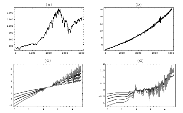
Figure 1: Time series of S$\&$P500 (a), model-generated prices (b), plot of $\log E[\mid x(t,\Delta t)\mid^{q}]$ against $\log[\Delta t]$ for S$\&$P500 (c) and simulations (d) respectively for $q+1=1,1.5,2,2.5,3$ top down at the left side.

under existence conditions given in [8]. Assuming that $x(t)=\log P(t)-\log P(0)$ Table (2) reports the $R^{2}$ of a regression of $\log E[\mid P(t,\Delta)\mid^{q}]$ against $\log\Delta(t)$ with $q+1=1,1.5,2,2.5,3$. $P$ is the daily closure of S$\&$P500 and the model-generated time series. Figure (1) reports the time series and the $\log$-$\log$ plot after normalizing by subtracting $\log E\mid x(t,\ log[10])\mid^{q}]$. Time intervals range from 1 to 100 days. There is no apparent crossover up to a scale of 100 days in the S$\&$P500 and the linear fit is very good, in accord with the behavior of a multifractal process. Crossover occurs in the simulations for values of $t$ between $e^{3}$ and $e^{4}$ and the fluctuations are more erratic than those of S$\&$P500. Such a behavior underlines the capability of the model to generate dynamics typical of a multifractal process, however the dynamics for the fundamental implies that price is mean-reverting around an exponenential trend, which in turn implies that crossover occurs for smaller time intervals than those of real time series. The introduction of stochastic noises or a feedback between fundamental and price determines more a realistic long-run behavior and scaling properties, as we will show for the latter case in Section 4.4.

4 Sensitivity analysis

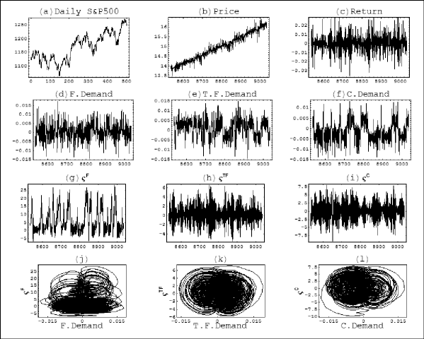
Figure 2: Time series of S$\&$P500 (a), price (b), returns(c), demand of fundamentalists (d), trend followers (e), contrarians (f), risk aversion of fundamentalists (g), trend followers (h), contrarians (i), projection of the phase space on planes $[D^{F},\varsigma^{F}]$ (j), $[D^{TF},\varsigma^{TF}]$ (k), $[D^{C},\varsigma^{C}]$ (l).

In this section we will first analyze the system dynamics and then we will study the variations in dynamics as some key parameters are changed. In Figure (2) there are depicted the time series of the last 500 observations of prices of S$\&$P500 and model, returns, demands, risk attitudes and the projections of the phase space on the planes $[D^{F},\varsigma^{F}]$, $[D^{TF},\varsigma^{TF}]$, $[D^{C},\varsigma^{C}]$. Tables (3,4,5) show statistics for different parameters values. The demands of technical traders switch between positive and negative phases, differently from the fundamentalist demand, which instead tends to move around zero. The presence of long phases of positive and negative demands of technical traders, together with the dynamics for the risk aversions may determine very large price oscillations in both directions. The increase in the fundamental value triggers a stock price increase due to the purchases by fundamentalists, which is reinforced by the action of trend followers. The demand of fundamentalists has smaller oscillations in the periods where the risk aversion is high, because a high risk aversion induces the fundamentalists not to open large positions if the stock is mispriced. Whereas the risk aversion of fundamentalists follows well defined trends and is on average positive, those of technical traders tends to oscillate around zero. As such, technical traders switch between phases in which they are risk averse and phases in which are risk seekers. The dynamics for the risk attitudes may be explained in the following way: let us assume that the price is rising and the demand of trend followers is positive and greater than $\sqrt{V^{TF}}$. Equation (11) implies that their risk aversion rises as well. The increase in price reduces the demand of fundamentalists and contrarians, but reinforces that of trend followers, which on the other hand tends to fall because of the increase in their risk aversion. Once the price falls, the demand of trend followers approaches zero (eventually becoming negative) and, as a consequence, their risk aversion falls. The dynamics are also the same in the case where the cycle is triggered by fundamentalists or contrarians. Risk attitudes may vary considerably even during phases in which the demands are almost steady. Indeed it is sufficient that the absolute value of the demand of investors type $i$ remains for a long time respectively above $\sqrt{V^{i}}$ to get a considerable change in risk aversion. The time derivatives of the risk attitudes tend to reach their lower bounds, which are respectively equal to $-\delta^{F}V^{F}$, $-\delta^{TF}V^{TF}$ and $-\delta^{C}V^{C}$, only when the demands are very close to zero.

4.1. Effects of changing the proportion of fundamentalists and technical traders. In order to analyze the effect of the proportion of fundamentalists and technical traders, we select values of $\alpha$ ranging from 0 to 1 and with a difference of 0.1 between a simulation and the next. If there are no fundamentalists or if their proportion is only ten percent, the price goes to infinity, because technical trading drives the price away from the fundamental. If $\alpha=0.1$ the fundamentalists are able to steer the price to the fundamental value, but prices are subject to large oscillations induced by technical traders. Such oscillations become larger and larger as time goes on. In fact larger departures from the fundamental value are needed for the fundamentalists to bring the price back close to the fundamental value. When $\alpha=0.2$ the departure from the fundamental value brings about long phases in which the fundamentalists go either long or short on the asset, determining in this way an increase in their risk aversion. This in turn implies a lower capability of offsetting technical traders. The overall demand of the latter presents long phases in which the demand is either positive or negative, phases in which it changes sign quickly and phases where the demands of contrarians and trend followers synchronize and offset each other. During phases of synchronization the system reduces by one dimension. When the technical demand is equal or close to zero, fundamentalists bring the price back close to the fundamental value. As a consequence of the fact that the total demand does not change sign for long periods, the price tends to follow a monotonic trajectory when it is far from the fundamental and to oscillate as it gets close to it. Thus, the synchronization of technical traders determines an intermittent behavior in the system with regular monotonic phases interrupted by chaotic bursts. The time series of fundamentalist and technical demands are depicted in Table (3). If $\alpha=0.3$ the proportion of fundamentalist is sufficiently high as to prevent technical trading from bringing about larger and larger departures from the fundamental value. The oscillations have anyway larger amplitudes than in the case where $\alpha=0.4$, and this in turn determines an increase in the variance and a decrease in the kurtosis. If fundamentalists account for half of the investors, the demand of technical traders is generally lower than in the baseline case because fundamental trading prevents strong changes in the price. This leaves little room for a persistent phase of fundamentalist demand and therefore fundamentalists are more likely to became risk seekers. The higher proportion of fundamentalists determines a more regular behavior of the system, as denoted by the decrease in kurtosis. If the fraction of fundamentalists is equal to or greater than sixty percent, the system no longer converges to a strange attractor, but to a quasi-periodic attractor, as denoted by the values of the Lyapunov exponents. If there are only fundamentalists the attractor becomes strange again and the Lyapunov exponent rises up to 0.53689, which would indicate a highly chaotic system. However the rise in the Lyapunov exponent is due to the increase in the amplitudes of the oscillations that in turn are due to the overreaction induced by the delayed reaction of fundamentalists, which brings price above (below) the fundamental price when the security is originally underpriced (overpriced).

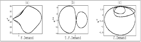
Figure 4: projection of the phase space on planes $[D^{F},\varsigma^{F}]$ (j), $[D^{TF},\varsigma^{TF}]$ (k), $[D^{C},\varsigma^{C}]$ (l) when $\lambda^{F}=190$.

4.2. Effects of changing the speed of expected price adjustment of fundamentalists. Increasing the speed reaction of fundamentalists brings about a decrease in the variance because the price tends to stay close to the fundamental. The system undergoes a global bifurcation as the parameter $\lambda^{F}$ is increased, indeed the dynamics show a cyclical behavior after a transient chaotic phase. This kind of transition, called attractor destruction, is a type of crisis-induced intermittency and has been investigated by [5] and [6]. However, for large values of $\lambda^{F}$ the attractor becomes strange again. Because of the presence of technical traders, which are affected by the changes in prices triggered by the fundamentalists, it is not possible to determine what the dynamics eventually are as the reaction speed of the fundamentalists is further increased. For instance, if $\lambda^{F}=190$ the dynamics are periodic, but if if $\lambda^{F}=300$ the attractor is strange, with a Lyapunov exponent of 0.240495. The projections of a limit cycle to which the system converges when $\lambda^{F}=190$ are represented in Figure (4)

4.3. Effects of switching between trend following and contrarian strategies. So far we have dealt with a model where the proportion between trend followers and contrarians are kept constant. If $z>0$ such proportions become path dependent. The higher the value of $z$, the higher the fraction of trend followers because this strategy is generally more profitable than the contrarian one, since price grows in the long run. Simulations for different values of $z$ show that a higher proportion of trend followers causes greater departures from the fundamental value triggering a reaction by all types of investors. Such dynamics bring about an increase in the variance and skewness of returns. Skewness tends to increase because overshooting is positive on average, since price tends to follow an exponentially growing fundamental. Kurtosis first tends to increase and then to decrease because the increase in variance for high values of $z$ determines that some returns previously in the tails of the distribution now approach the center.

4.4. Effects of introducing a feedback between price and fundamental. We will assume now that the fundamental value is affected by the asset price. The economic rationale is that a higher price boosts consumption and, as a consequence, the real economy as a whole. We assume that the dynamics of the fundamental follows the differential equation:

$$\frac{\dot{F}(t)}{F(t)}=g+m\frac{P(t)}{F(t)}\,\,;\,m=0.5.$$ (15)

The introduction of this kind of feedback induces a unit root behavior in the price time series with scaling properties very to those of S&P500. This is apparent from Figure (5) where there are reported the simulated time series and the plot of $\log E[\mid x(t,\Delta t)\mid^{q}]$ against $\log[\Delta t]$ and from the regression analysis. Indeed the $R^{2}$ values are $R^{2}(q+1=1)=0.986382$, $R^{2}(q+1=1.5)=0.987099$, $R^{2}(q+1=2)=0.987352$, $R^{2}(q+1=2.5)=0.987521$, $R^{2}(q+1=3)=0.987641$.

5 Conclusion

In this paper we have outlined a continuous time deterministic model of a financial market with heterogeneous interacting agents. The dynamical system is able to generate some stylized facts present in real markets, even in a purely deterministic setting: excess kurtosis, volatility clustering and long memory. Even in the case where fundamentalists are the only agents present in the market, they are unable to drive the price back to the fundamental on a steady state trajectory. Moreover, the increase in the fundamentalist reaction speed may even increase the disorder in the system, because the fundamentalists trigger a strong response of technical traders. It may also be possible that, when the fraction of fundamentalists is low, trend followers and contrarians give rise to synchronization in the system, bringing about a dramatic change in the dynamics. The introduction of an evolutionary switching between technical traders leads to an increase in the volatility and in the kurtosis, provided that the speed of switching is not too high because otherwise the increase in the variance makes it less likely that returns will fall in the tails of the distributions. Further research will take into account more realistic distribution functions for the agents, the introduction of stochastic disturbances and a deeper investigation of the interaction between price and fundamental.

	Mean	Variance	Skewness	Kurtosis	Jar.Bera	Lyap.exp.
S$\&$P500	0.0003597	0.0001026	-0.0146	6.700	421.9
Model	0.0003617	0.0001100	-0.0293	6.115	1632	0.2500

Table 1: Statistics of S$\&$P500 and simulated time series.

} $R^{2}$ $q+1=1$ $q+1=1.5$ $q+1=2$ $q+1=2.5$ $q+1=3$ S$\&$P500 0.9870 0.9854 0.9820 0.9771 0.9707 Model 0.848 0.8287 0.7980 0.7492 0.6769

Table 2: $R^{2}$ of $\log E[\mid P(t,\Delta)\mid^{q}]$ regressed against $\log\Delta(t)$

$\alpha$	Mean	Variance	Skewness	Kurtosis	Jar.Bera	Lyap.exp.
0.2	0.004344	0.00527	0.7748	3.330	421.9
0.3	0.00088	0.001154	0.1378	4.107	218	0.269
0.4	0.0003631	0.0001100	-0.02968	6.115	1631	0.2500
0.5	0.0003317	0.00004472	0.2504	5.153	821.1	0.1718
0.6	0.0004837	0.0003519	0.02186	1.595	331.9	0.1118
0.7	0.0005229	0.0004317	0.01568	1.514	370.8	0.03375
0.8	0.000437	0.0002437	0.01894	1.774	252.7	0.03621
0.9	0.0004538	0.0002923	0.130	6.439	1999	0.03992
1	0.0005047	0.0003806	0.6031	22.05	61275	0.536

Table 3: Statistics of the simulated time series as $\alpha$ varies from 0.2 to 1.

$\lambda^{F}$	Mean	Variance	Skewness	Kurtosis	Jar.Bera	Lyap.exp.
19/15	0.0005586	0.000495	0.1102	3.876	137.1	0.2446
38/15	0.0004701	0.0003267	0.134	4.030	190.4	0.2222
57/15	0.0004320	0.0002342	-0.01053	3.660	73.46	0.2639
76/15	0.0003842	0.0001536	0.02541	3.694	81.51	0.248
95/15	0.0003631	0.0001100	-0.02968	6.115	1631	0.2500
114/15	0.0003550	0.00009703	0.05448	6.398	1942	0.2242
133/15	0.0003584	0.0001020	0.1003	4.627	451.7	0.05490
152/15	0.0003565	0.0001000	0.04832	4.922	622.6	0.2196
171/15	0.0003468	0.00007810	-0.155	1.819	250.6	0.2118
190/15	0.00034	0.00007369	0.0004368	5.462	1019	0.002247
190	0.0003355	0.00005448	-0.06733	1.931	194.9	0.07157
300	0.0004425	0.0002832	0.2366	3.589	96.09	0.2404

Table 4: Statistics of the simulated time series as $\lambda^{F}$ varies from 19/15 to 190/15 and $\lambda^{F}=190\,;\,300$.

z	Mean	Variance	Skewness	Kurtosis	Jar.Bera
5	0.000359	0.0001042	0.06756	6.268	1798
10	0.0003588	0.0001083	0.1103	5.439	1007
20	0.0003643	0.0001146	0.08794	5.663	1197
30	0.0003838	0.0001539	0.1881	10.533	9560
40	0.0003900	0.0001465	0.1540	8.243	4635
60	0.0004234	0.0002252	0.3276	7.064	2848
80	0.0004667	0.0003244	0.3391	7.810	3965

Table 5: Statistics of the simulated time series as $z$ varies from 5 to 80.

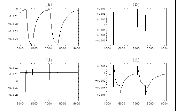
Figure 3: Total demand of fundamentalists (a), trend followers (b), contrarians (c) and market excess demand (d) when $\alpha=0.2$.

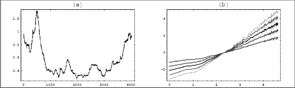
Figure 5: Time series of the price (a) and plot of $\log E[\mid x(t,\Delta t)\mid^{q}]$ against $\log[\Delta t]$ with price-fundamental feedback (b).

References

- [1] A. Beja and M. Goldman, J.Finance 35 (1980), 235-248.
- [2] W. A. Brock and C. H. Hommes, Heteroeneous beleiefs and routes to chaos in a simple asset pricing model, Journal of Economic Dynamics and Control 22 (1998), 1235-1274.
- [3] C. Chiarella, The dynamics of speculative behavior, Annals of Operations Research 37 (1992), 101-124
- [4] C. Chiarella and X.Z. He, Asset Pricing and wealth dynamics under heterogeneous expectations, Quant. Finance 1 (2001), 509-526.
- [5] C. Grebogi, E. Ott and J.A. Yorke, Critical exponent of chaotic transientin nonlinear dynamical systems, Phys. Rev. Lett. 57 (1986), 1284-1287.
- [6] C. Grebogi, E. Ott, F. Romeiras, and J.A. Yorke, Critical exponent for crisis-induced intermittency, Phys. Rev. A 36 (1987), 5365-5380.
- [7] W.G. Hoover, Canonical dynamics: equilibrium phase-space distributions, Phys. Rev. A 31 (1985), 1695-1697.
- [8] B. Mandelbrot, A. Fisher, and L. Calvet, A multifractal model of asset returns, Working paper, Cowles Foundation Discussion Papers 1164 (1997).
- [9] S. Nosè, A molecular dynamics method for simulation in the canonical ensemble, J. Chem. Phys. 81 (1984a), 511-519.
- [10] S. Nosè, Molecular dynamics simulations, Progress of Theoretical Physics Supplement 103 (1984b), 1-49.
- [11] F. Westerhoff, Greed, fear and stock market dynamics, Physica A 343C (2004a), 635-642.
- [12] F. Westerhoff, Market depth and price dynamics: a note, Int. J. Mod. Phys. C 15 (2004b), 1005-1012.
- [13] S. Thurner, E.J. Dockner, A. Gaunersdorfer, S. Thurner, E.J. Dockner, and A. Gaunersdorfer, Asset price dynamics in a model of investors operating on different time horizon, Working paper, SFB-WP 93, University of Vienna (2002).