Synergetic Analysis of the Häussler-von der Malsburg Equations
for Manifolds of Arbitrary Geometry

Abstract

We generalize a model of Häussler and von der Malsburg which describes the self-organized generation of retinotopic projections between two one-dimensional discrete cell arrays on the basis of cooperative and competitive interactions of the individual synaptic contacts. Our generalized model is independent of the special geometry of the cell arrays and describes the temporal evolution of the connection weights between cells on different manifolds. By linearizing the equations of evolution around the stationary uniform state we determine the critical global growth rate for synapses onto the tectum where an instability arises. Within a nonlinear analysis we use then the methods of synergetics to adiabatically eliminate the stable modes near the instability. The resulting order parameter equations describe the emergence of retinotopic projections from initially undifferentiated mappings independent of dimension and geometry.

I Introduction

An important part of the visual system of vertebrate animals are the neural connections between the eye and the brain. At an initial stage of ontogenesis the ganglion cells of the retina have random synaptic contacts with the tectum, a part of the brain which plays an important role in processing optical information. In the adult animal, however, neighboring retinal cells project onto neighboring cells of the tectum (see Figure 1). Further examples of these so-called retinotopic projections are established between the retina and the corpus geniculatum laterale as well as the visual cortex, respectively kandel . This conservation of neighborhood relations is also realized in many other neural connections between different cell sheets. For instance, the formation of ordered projections between the mechanical receptors in the skin and the somatosensorial cortex is called somatotopy. An even more abstract topological projection arises when the spatially resolved detection of similar frequencies in the ear are projected onto neighboring cells of the auditorial cortex. A further notable neural map in the auditory system was discovered in the brain of the owl, where neighboring cells of the Nucleus mesencephalicus lateralis dorsalis (MLD) are excited by neighboring space areas, i.e. every space point is represented by a small zone of the MLD knudsen . The variety of examples suggest that there must be some underlying general mechanism for rearranging the initially disordered synaptic contacts into topological projections.

In the early 1940s, Sperry performed a series of pioneering experiments in the visual system of frogs and goldfish sperry1 ; sperry2 . Fish and amphibians can regenerate axonal tracts in their central nervous system, in contrast to mammals, birds and reptiles. Sperry crushed the optical nerve and found that retinal axons reestablished the previous retinotopically ordered pattern of connections in the tectum. Then in the early 1960s Sperry presented his chemoaffinity hypothesis which proposed that the retinotectal map is set up on the basis of chemical markers carried by the cells sperry3 . However, experiments over several decades have shown that the formation of retinotectal maps cannot be explained by this gradient matching alone goodhill .

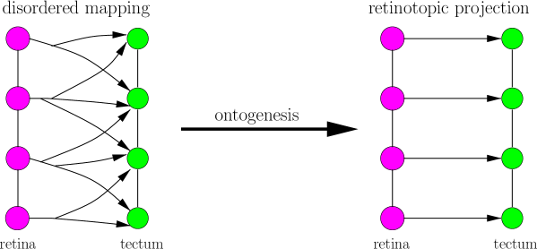
Figure 1: In the course of ontogenesis originally disordered mappings between retina and tectum evolve into ordered projections.

The group of von der Malsburg suggested that these ontogenetic processes result from self-organization. The basic notion in their theory is the following: Once a fibre has already grown from the retina to the tectum, the fibre moves along by strengthening its contacts in some parts of its ramification and by weakening them in others. It is assumed that these modifications are governed by two contradictory rules Malsburg1 ; Malsburg2 : on the one hand, synaptic contacts on neighboring tectal cells stemming from fibres of the same retinal region support each other to be strengthened. On the other hand, the contacts starting from one retinal cell or ending at one tectal cell compete with each other. In the case that retina and tectum are treated as one-dimensional discrete cell arrays, extensive computer simulations have shown that a system based on these ideas of cooperativity and competition establishes, indeed, retinotopy as the final configuration Malsburg2 . This finding was confirmed by a detailed analytical treatment of Häussler and von der Malsburg Malsburg3 where the self-organized formation of the synaptic connections between retina and tectum is described by an appropriate system of ordinary differential equations. Applying the methods of synergetics Haken1 ; Haken2 for one-dimensional discrete cell arrays, they succeeded in classifying the possible retinotopic projections and to discuss the criteria which determine their emergence. The more complicated case of continuously distributed cells on a spherical shell was partially discussed in Ref. Malsburg4 .

It is the purpose of this paper to follow the outline of Ref. Bochum and generalize the original approach by elaborating a model for the self-organized formation of retinotopic projections which is independent of the special geometry and dimension of the cell sheets. There are three essential reasons which motivate this more general approach. First, neurons usually do not establish 1-dimensional arrays but 2- or 3-dimensional networks. Hence the 1-dimensional model of Häussler and von der Malsburg can only serve as a simplistic approximation of the real situation. Secondly, we want to include cell sheets of different extent, which is a more realistic assumption than neural sheets with the same number of cells. The third reason is that a general model is able to reveal what is generic, i.e. what is independent of the special geometry of the problem. Thus, here we generalize the Häussler equations to continuous manifolds of arbitrary geometry. By doing so, we proceed in a phenomenological manner and relegate a microscopic derivation of the underlying equations to future research.

It should be emphasized that our main objective is not the biological modelling of retinotopy. Instead of that our considerations are devoted to the analysis of the dynamics of the nonlinear Häussler equations by using mathematical methods from nonlinear dynamics and synergetics. For the more biological aspects of retinotopy and the vast progress in modelling various retinotopically ordered projections during the last twenty years we refer the reader to the reviews goodhill ; goodhill2 ; swindale .

In Section II we present the general framework of our model and introduce the equations of evolution for the connection weights between retina and tectum. We then perform in Section III a linear stability analysis for the equations of evolution around the stationary uniform state and discuss under which circumstances an instability arises. In Section IV we apply the methods of synergetics, and elaborate within a nonlinear analysis that the adiabatic elimination of the fast evolving degrees of freedom leads to effective equations of evolution for the slow evolving order parameters. They approximately describe the dynamics near the instability where an increase of the uniform growth rate of new synapses onto the tectum beyond a critical value converts an initially disordered mapping into a retinotopic projection. Finally, Section V and VI provide a summary and an outlook.

II General Model

In this section we summarize the basic assumptions of our general model.

II.1 Manifolds and Their Properties

We start with representing retina ($R$) and tectum ($T$) by general manifolds ${\cal M}_{T}$ and ${\cal M}_{R}$, respectively. In the framework of an embedding of these manifolds in an Euclidean space of dimension $D$, the coordinates $x_{R}$, $x_{T}$ of the corresponding cells can be represented by

$$x_{R}=(x_{R}^{1},x_{R}^{2},\ldots,x_{R}^{D})\,,\qquad x_{R}\in{\cal M}_{R}\,;\hskip 28.45274ptx_{T}=(x_{T}^{1},x_{T}^{2},\ldots,x_{T}^{D})\,,\qquad x_{T}\in{\cal M}_{T}\,.$$ (1)

In the following we need measures of distance, i.e. metrics $g_{\mu\nu}^{R}$, $g_{\mu\nu}^{T}$ on the manifolds. The intrinsic coordinates of the $d$-dimensional manifolds ${\cal M}_{R}$, ${\cal M}_{T}$ are denoted by $r^{\mu}$, $t^{\mu}$. Thus, the vectors (1) of the Euclidean embedding space can be parametrized according to $x_{R}=x_{R}(r^{\mu})$, $x_{T}=x_{T}(t^{\mu})$. With the covariant metric tensors

$$g_{\mu\nu}^{R}=\frac{\partial x_{R}}{\partial r^{\mu}}\,\frac{\partial x_{R}}{\partial r^{\nu}}\,,\quad g_{\mu\nu}^{T}=\frac{\partial x_{T}}{\partial t^{\mu}}\,\frac{\partial x_{T}}{\partial t^{\nu}}$$ (2)

the line elements on the manifolds are given by $(ds_{R})^{2}=g_{\mu\nu}^{R}dr^{\mu}dr^{\nu}\,,\,(ds_{T})^{2}=g_{\mu\nu}^{T}dt^{\mu}dt^{\nu}\,.$ The geodetic distances between two points of the manifolds read

$$s_{rr^{\prime}}^{R}=\int\limits_{r^{\prime}}^{r}\!\!\sqrt{g_{\mu\nu}^{R}\,dr^{\mu}dr^{\nu}}\,,\qquad s_{tt^{\prime}}^{T}=\int\limits_{t^{\prime}}^{t}\!\!\sqrt{g_{\mu\nu}^{T}\,dt^{\mu}dt^{\nu}}\,.$$ (3)

We define a measure for the magnitudes of the manifolds by

$$M_{T}=\int\!dt\,,\qquad M_{R}=\int\!dr\,,$$ (4)

where we integrate over all elements of ${\cal M}_{T}$, ${\cal M}_{R}$. We characterize the neural connectivity within each manifold ${\cal M}_{T}$, ${\cal M}_{R}$ by cooperativity functions $c_{T}(t,t^{\prime})$, $c_{R}(r,r^{\prime})$. In lack of any theory for the cooperativity functions we regard them as time-independent, given properties of the manifolds which are only limited by certain global plausible constraints. We assume that the cooperativity functions are positive

$$c_{T}(t,t^{\prime})\geq 0\,,\qquad c_{R}(r,r^{\prime})\geq 0\,,$$ (5)

that they are symmetric with respect to their arguments

$$c_{T}(t,t^{\prime})=c_{T}(t^{\prime},t),\qquad c_{R}(r,r^{\prime})=c_{R}(r^{\prime},r)\,,$$ (6)

and that they fulfill the normalization conditions

$$\int\!dt^{\prime}\,c_{T}(t,t^{\prime})=1,\qquad\int\!dr^{\prime}\,c_{R}(r,r^{\prime})=1\,.$$ (7)

Furthermore, it is neurophysiologically reasonable to assume that the cooperativity functions $c_{T}(t,t^{\prime})$, $c_{R}(r,r^{\prime})$ are larger when the distance between the points $t,t^{\prime}$ and $r,r^{\prime}$ is smaller. This condition of monotonically decreasing cooperativity functions can be written as

$$c_{T}(t,t^{\prime})>c_{T}(t,t^{\prime\prime})\,\mbox{ if }\,(s_{tt^{\prime}}^{T})^{2}<(s_{tt^{\prime\prime}}^{T})^{2}\,,\quad c_{R}(r,r^{\prime})>c_{R}(r,r^{\prime\prime})\,\mbox{ if }\,(s_{rr^{\prime}}^{R})^{2}<(s_{rr^{\prime\prime}}^{R})^{2}\,.$$ (8)

II.2 Equations of Evolution

The neural connections between retina and tectum are described by a connection weight $w(t,r)$ for every ordered pair $(t,r)$ with $t\in{\cal M}_{T},\,r\in{\cal M}_{R}$. In this paper we are interested in the temporal evolution of the connection weight $w(t,r)$ which is essentially determined by the given cooperativity functions $c_{T}(t,t^{\prime})$, $c_{R}(r,r^{\prime})$ of the manifolds ${\cal M}_{T}$, ${\cal M}_{R}$. To this end we generalize a former ansatz of Häussler and von der Malsburg Malsburg3 and assume that the evolution is governed by the following system of ordinary differential equations thesis :

$$\dot{w}(t,r) = \alpha+w(t,r)\,\int\!dt^{\prime}\,\int\!dr^{\prime}c_{T}(t,t^{\prime})\,c_{R}(r,r^{\prime})\,w(t^{\prime},r^{\prime})$$ (9)

$$-\frac{w(t,r)}{2M_{T}}\hskip 2.84526pt\int\!dt^{\prime}\left[\alpha+w(t^{\prime},r)\,\int\!dt^{\prime\prime}\,\int\!dr^{\prime}c_{T}(t^{\prime},t^{\prime\prime})\,c_{R}(r,r^{\prime})\,w(t^{\prime\prime},r^{\prime})\right]$$

$$-\frac{w(t,r)}{2M_{R}}\hskip 2.84526pt\int\!dr^{\prime}\left[\alpha+w(t,r^{\prime})\,\int\!dt^{\prime}\,\int\!dr^{\prime\prime}c_{T}(t,t^{\prime})\,c_{R}(r^{\prime},r^{\prime\prime})\,w(t^{\prime},r^{\prime\prime})\right]\,.$$

Here $\alpha$ denotes the uniform growth-rate of new synapses onto the tectum, which will be the control parameter of our system. These equations of evolution represent a balance between different cooperating and competing processes. To see this, we define the growth rate between the cells at $r$ and $t$

$$f(t,r,w)=\alpha+w(t,r)\int\!dt^{\prime}\,\int\!dr^{\prime}c_{T}(t,t^{\prime})\,c_{R}(r,r^{\prime})\,w(t^{\prime},r^{\prime})\,,$$ (10)

so that the generalized Häussler equations (9) reduce to

$$\dot{w}(t,r)=f(t,r,w)-\frac{w(t,r)}{2M_{T}}\hskip 5.69054pt\int\!dt^{\prime}f(t^{\prime},r,w)-\frac{w(t,r)}{2M_{R}}\hskip 5.69054pt\int\!dr^{\prime}f(t,r^{\prime},w)\,.$$ (11)

The cooperative contribution of the connection between $r^{\prime}$ and $t^{\prime}$ to the growth rate between $r$ and $t$ is given by the product $w(t,r)c_{T}(t,t^{\prime})c_{R}(r,r^{\prime})w(t^{\prime},r^{\prime})$ as shown in Figure 2a. Therefore, this cooperative contribution is integrated with respect to $r^{\prime}$, $t^{\prime}$ and added to the uniform growth rate $\alpha$ to yield the total growth rate (10) between $r$ and $t$. Apart from this cooperative term in the equations of evolution (11), the remaining terms describe competitive processes. The second term accounts for the fact that growth rates between $r$ and $t^{\prime}$ compete with the connections between $r$ and $t$ (see Figure 2b). Correspondingly, the third term describes the competition of the growth rates between $r^{\prime}$ and $t$ with the connections between $r$ and $t$ (see Figure 2c).

a)

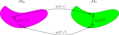
b)

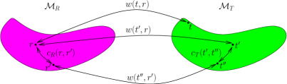
c)

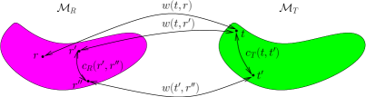
Figure 2: Illustrations for the respective contributions to the generalized Häussler equations (11). Discussion see text.

II.3 Lower Limits for the Connection Strength

Now we show that the evolution of the system due to the generalized Häussler equations (9) leads to a lower bound for the connection weight. To this end we assume the inequality

$$0\leq w(t,r)\leq W$$ (12)

to be fulfilled for some initial configuration. Then we conclude that the quantity

$$C(t,r,w)=\int\!dt^{\prime}\int\!dr^{\prime}c_{T}(t,t^{\prime})\,c_{R}(r,r^{\prime})\,w(t^{\prime},r^{\prime})$$ (13)

is positive as both the cooperativity functions $c_{T}(t,t^{\prime})$, $c_{R}(r,r^{\prime})$ and the connection weight $w(t^{\prime},r^{\prime})$ are positive due to (5) and (12). On the other hand we read off from the normalization of the cooperativity functions (7) that $C(t,r,w)$ cannot be larger than $W$: $0\leq C(t,r,w)\leq W$. With this we can find a lower bound for $\dot{w}(t,r)$ as follows. The growth rate (10) reads together with (13): $f(t,r,w)=\alpha+w(t,r)\,C(t,r,w)$. It can be minimized by setting $C(t,r,w)=0$, i.e.

$$f(t,r,w)_{\rm min}=\alpha\,,$$ (14)

whereas its maximum value follows from $C(t,r,w)=W$:

$$f(t,r,w)_{\rm max}=\alpha+W^{2}\,.$$ (15)

To obtain a lower bound for $\dot{w}(t,r)$ in the Häussler equations (11), we insert the minimum (14) of the growth rate for the cooperative first term and its maximum (15) for the remaining competitive terms:

$$\dot{w}(t,r)_{\rm min} = \alpha-w(t,r)\left(\alpha+W^{2}\right)\,.$$ (16)

Hence a small but positive $w(t,r)$ is prevented by a positive rate $\alpha$ from becoming zero. In this way we can conclude that the connection weight $w(t,r)$ is positive, when the inequality (12) is valid in an initial configuration. All further investigations will concentrate on solutions of the Häussler equations (9) with $w(t,r)\geq 0$. Note that, in particular, the growth rates (10) for such configurations are positive.

II.4 Complete Orthonormal System

To perform both a linear and a nonlinear analysis of the underlying Häussler equations (9) we need a complete orthonormal system for both manifolds ${\cal M}_{T}$ and ${\cal M}_{R}$. With the help of the contravariant components $g^{\lambda\mu}_{T}$, $g^{\lambda\mu}_{R}$ of the metric introduced in Section II.1 we define the respective Laplace-Beltrami operators on the manifolds

$$\Delta_{T}=\frac{1}{\sqrt{g_{T}}}\,\partial_{\lambda}\left(g^{\lambda\mu}_{T}\sqrt{g_{T}}\,\partial_{\mu}\right)\,,\hskip 28.45274pt\Delta_{R}=\frac{1}{\sqrt{g_{R}}}\,\partial_{\lambda}\left(g^{\lambda\mu}_{R}\sqrt{g_{R}}\,\partial_{\mu}\right)\,,$$ (17)

where $g_{T},g_{R}$ represent the determinants of the covariant components $g_{\lambda\mu}^{T}$, $g_{\lambda\mu}^{R}$ of the metric. The Laplace-Beltrami operators allow to introduce a complete orthonormal system by their eigenfunctions $\psi_{\lambda_{T}}(t)$, $\psi_{\lambda_{R}}(r)$ according to

$$\Delta_{T}\,\psi_{\lambda_{T}}(t)=\chi^{T}_{\lambda_{T}}\,\psi_{\lambda_{T}}(t)\,,\hskip 28.45274pt\Delta_{R}\,\psi_{\lambda_{R}}(r)=\chi^{R}_{\lambda_{R}}\,\psi_{\lambda_{R}}(r)\,.$$ (18)

Here $\lambda_{T}$, $\lambda_{R}$ denote discrete or continuous numbers which parameterize the eigenvalues $\chi^{T}_{\lambda_{T}}$, $\chi^{R}_{\lambda_{R}}$ of the Laplace-Beltrami operators which could be degenerate. By construction, they fulfill the orthonormality relations

$$\int\!dt\,\psi_{\lambda_{T}}(t)\psi_{\lambda_{T}^{\prime}}^{*}(t)=\delta_{\lambda_{T}\lambda_{T}^{\prime}}\,,\hskip 28.45274pt\int\!dr\,\psi_{\lambda_{R}}(r)\psi_{\lambda_{R}^{\prime}}^{*}(r)=\delta_{\lambda_{R}\lambda_{R}^{\prime}}\,,$$ (19)

and the completeness relations

$$\sum_{\hskip 5.69054pt{}_{\lambda_{T}}}\psi_{\lambda_{T}}(t)\psi_{\lambda_{T}}^{*}(t^{\prime})=\delta(t-t^{\prime})\,,\hskip 28.45274pt\sum_{\hskip 5.69054pt{\lambda_{R}}}\psi_{\lambda_{R}}(r)\psi_{\lambda_{R}}^{*}(r^{\prime})=\delta(r-r^{\prime})\,.$$ (20)

Note that the explicit form (17) of the Laplace-Beltrami operators enforces the eigenvalues $\chi^{T}_{\lambda_{T}=0}=0\,,\chi^{R}_{\lambda_{R}=0}=0$ with the constant eigenfunctions

$$\psi_{\lambda_{T}=0}(t)=\frac{1}{\sqrt{M_{T}}}\,,\hskip 28.45274pt\psi_{\lambda_{R}=0}(r)=\frac{1}{\sqrt{M_{R}}}$$ (21)

because of (4) and the orthonormality relations (19). The cooperativity functions can be expanded in terms of the eigenfunctions according to

$$c_{T}(t,t^{\prime})=\sum_{\hskip 5.69054pt{\lambda_{T}}}\sum_{\hskip 5.69054pt{\lambda_{T}^{\prime}}}F_{\lambda_{T}\lambda_{T}^{\prime}}\psi_{\lambda_{T}}(t)\psi_{\lambda_{T}^{\prime}}^{*}(t^{\prime})\,,\quad c_{R}(r,r^{\prime})=\sum_{\hskip 5.69054pt{\lambda_{R}}}\sum_{\hskip 5.69054pt{\lambda_{R}^{\prime}}}F_{\lambda_{R}\lambda_{R}^{\prime}}\psi_{\lambda_{R}}(r)\psi_{\lambda_{R}^{\prime}}^{*}(r^{\prime})\,.$$ (22)

In the following we assume for the sake of simplicity that the corresponding expansion coefficients are diagonal $F_{\lambda_{T}\lambda_{T}^{\prime}}=f_{\lambda_{T}}\delta_{\lambda_{T}\lambda_{T}^{\prime}}\,,\,F_{\lambda_{R}\lambda_{R}^{\prime}}=f_{\lambda_{R}}\delta_{\lambda_{R}\lambda_{R}^{\prime}}\,,$ so we have

$$c_{T}(t,t^{\prime})=\sum_{\hskip 5.69054pt{\lambda_{T}}}f_{\lambda_{T}}\psi_{\lambda_{T}}(t)\psi_{\lambda_{T}}^{*}(t^{\prime})\,,\hskip 28.45274ptc_{R}(r,r^{\prime})=\sum_{\hskip 5.69054pt{\lambda_{R}}}f_{\lambda_{R}}\psi_{\lambda_{R}}(r)\psi_{\lambda_{R}}^{*}(r^{\prime})\,.$$ (23)

Thus, $\psi_{\lambda_{T}}(t)$, $\psi_{\lambda_{R}}(r)$ are not only eigenfunctions of the Laplace-Beltrami operators as in (18) but also eigenfunctions of the cooperativity functions according to

$$\int\!dt^{\prime}\,c_{T}(t,t^{\prime})\,\psi_{\lambda_{T}}(t^{\prime})=f_{\lambda_{T}}\,\psi_{\lambda_{T}}(t)\,,\hskip 28.45274pt\int\!dr^{\prime}\,c_{R}(r,r^{\prime})\,\psi_{\lambda_{R}}(r^{\prime})=f_{\lambda_{R}}\,\psi_{\lambda_{R}}(r)\,.$$ (24)

Note that the normalization of the cooperativity functions (7) and the orthonormalization relations (19) lead to the constraints $f_{\lambda_{T}=0}=f_{\lambda_{R}=0}=1\,.$

III Linear Stability Analysis

Now we employ the methods of synergetics Haken1 ; Haken2 and investigate the underlying equations of evolution (9) in the vicinity of the stationary uniform solution. Inserting the ansatz $w(t,r)=w_{0}$ into the Häussler equations (9), we take into account (4) as well as the normalization of the cooperativity functions (7). By doing so, we deduce $w_{0}=1$. Let us introduce the deviation from this stationary uniform solution $v(t,r)=w(t,r)-1\,,$ and rewrite the Häussler equations (9). Defining the linear operators

$$\hat{C}(t,r,x) = \int\!dt^{\prime}\int\!dr^{\prime}\,c_{T}(t,t^{\prime})\,c_{R}(r,r^{\prime})\,x(t^{\prime},r^{\prime})\,,$$ (25)

$$\hat{B}(t,r,x) = \frac{1}{2M_{T}}\int\!dt^{\prime}\,x(t^{\prime},r)+\frac{1}{2M_{R}}\int\!dr^{\prime}\,x(t,r^{\prime})\,,$$ (26)

the resulting equations of evolution assume the form

$$\dot{v}(t,r)=\hat{L}(t,r,v)+\hat{Q}(t,r,v)+\hat{K}(t,r,v)\,.$$ (27)

Here the linear, quadratic, and cubic terms, respectively, are given by

$$\hat{L}(t,r,v) = -\alpha v+\hat{C}(t,r,v)-\hat{B}(t,r,v)-\hat{B}(t,r,\hat{C}(t,r,v))\,,$$ (28)

$$\hat{Q}(t,r,v) = v\,\left(\hat{C}(t,r,v)-\hat{B}(t,r,v)-\hat{B}(t,r,\hat{C}(t,r,v))\right)-\hat{B}\left(t,r,v\,\hat{C}(t,r,v)\right)\,,$$ (29)

$$\hat{K}(t,r,v) = -v\,\hat{B}\left(t,r,v\,\hat{C}(t,r,v)\right)\,.$$ (30)

To analyze the stability of the stationary uniform solution we neglect for the time being the nonlinear terms in (27) and investigate the linear problem

$$\dot{v}(t,r)=\hat{L}(t,r,v)\,.$$ (31)

Solutions of (31) depend exponentially on the time $\tau$, $v(t,r)=v_{\lambda_{T}\lambda_{R}}(t,r)\exp\left(\Lambda_{\lambda_{T}\lambda_{R}}\,\tau\right)$ with $v_{\lambda_{T}\lambda_{R}}$ and $\Lambda_{\lambda_{T}\lambda_{R}}$ denoting the eigenfunctions and eigenvalues of the linear operator $\hat{L}$:

$$\hat{L}\left(t,r,v_{\lambda_{T}\lambda_{R}}\right)=\Lambda_{\lambda_{T}\lambda_{R}}\,v_{\lambda_{T}\lambda_{R}}(t,r)\,.$$ (32)

Now we use the complete and orthonormal system on the manifolds ${\cal M}_{T}$, ${\cal M}_{R}$, which have been defined in Section II.4, and show that the eigenfunctions of $\hat{L}$ are products of the form

$$v_{\lambda_{T}\lambda_{R}}(t,r)=\psi_{\lambda_{T}}(t)\,\psi_{\lambda_{R}}(r)\,.$$ (33)

Indeed, when the operator (25) acts on (33), the expansion of the cooperativity functions (23) leads, together with the orthonormality relations (19), to

$$\hat{C}(t,r,v_{\lambda_{T}\lambda_{R}})=f_{\lambda_{T}}\,f_{\lambda_{R}}\,v_{\lambda_{T}\lambda_{R}}(t,r)\,.$$ (34)

Thus, the operator $\hat{C}$ has the eigenfunctions $v_{\lambda_{T}\lambda_{R}}(t,r)$ with the eigenvalues $f_{\lambda_{T}}f_{\lambda_{R}}$. In a similar way we obtain for the operator (26):

$$\hat{B}(t,r,v_{\lambda_{T}\lambda_{R}})=\left\{\begin{array}[]{ccc}v_{\lambda_{T}\lambda_{R}}&&\lambda_{T}=\lambda_{R}=0\,,\\[5.69054pt] v_{\lambda_{T}\lambda_{R}}/2&&\lambda_{T}=0\,,\lambda_{R}\not=0;\lambda_{R}=0\,,\lambda_{T}\not=0\,,\\[5.69054pt] 0&&\mbox{otherwise}\,.\end{array}\right.$$ (35)

Combining the eigenvalue problems (34), (35) for $\hat{C}$ and $\hat{B}$, we find

$$\hat{B}\left(t,r,\hat{C}(v_{\lambda_{T}\lambda_{R}})\right)=\left\{\begin{array}[]{ccc}f_{\lambda_{T}}f_{\lambda_{R}}v_{\lambda_{T}\lambda_{R}}&&\lambda_{T}=\lambda_{R}=0\vspace{0.15cm}\,,\\ f_{\lambda_{T}}f_{\lambda_{R}}v_{\lambda_{T}\lambda_{R}}/2&&\lambda_{T}=0\,,\lambda_{R}\not=0;\lambda_{R}=0\,,\lambda_{T}\not=0\vspace{0.15cm}\,,\\ 0&&\mbox{otherwise}\,.\end{array}\right.$$ (39)

Thus, we conclude from (34)–(39) that the linear operator $\hat{L}$ fulfills the eigenvalue problem (32) with the eigenfunctions (33) and the eigenvalues

$$\Lambda_{\lambda_{T}\lambda_{R}}=\left\{\begin{array}[]{ccc}-\alpha-1&&\lambda_{T}=\lambda_{R}=0\vspace{0.15cm}\,,\\ -\alpha+(f_{\lambda_{T}}f_{\lambda_{R}}-1)/2&&\lambda_{T}=0\,,\lambda_{R}\not=0;\lambda_{R}=0\,,\lambda_{T}\not=0\vspace{0.15cm}\,,\\ -\alpha+f_{\lambda_{T}}f_{\lambda_{R}}&&\mbox{otherwise}\,.\end{array}\right.$$ (40)

By changing the uniform growth rate $\alpha$ in a suitable way, the real parts of some eigenvalues (40) become positive and the system can be driven to the neighborhood of an instability. Which eigenvalues (40) become unstable in general depends on the respective values of the given expansion coefficients $f_{\lambda_{T}}$, $f_{\lambda_{R}}$. The situation simplifies, however, if we follow Ref. Malsburg3 and assume that the absolute values of the expansion coefficients $f_{\lambda_{T}}$, $f_{\lambda_{R}}$ are equal or smaller than the normalization value $f_{0}=1$: $|f_{\lambda_{T}}|\leq 1\,,|f_{\lambda_{R}}|\leq 1$. Then the eigenvalue in (40) with the largest real part is given by some parameters $\lambda_{T}^{u},\lambda_{R}^{u}$ with $\Lambda_{\rm max}=\Lambda_{\lambda_{T}^{u}\lambda_{R}^{u}}=-\alpha+f_{\lambda_{T}^{u}}f_{\lambda_{R}^{u}}$. Thus, the linear stability analysis reveals that the instability arises at the critical uniform growth rate

$$\alpha_{c}=\mbox{Re}\,(f_{\lambda_{T}^{u}}f_{\lambda_{R}^{u}})$$ (41)

and that its neighborhood is characterized by

$$\mbox{Re}\,(\Lambda_{\lambda_{T}^{u}\lambda_{R}^{u}})\approx 0\,;\hskip 28.45274pt\mbox{Re}\,(\Lambda_{\lambda_{T}\lambda_{R}})\ll 0\,,\quad(\lambda_{T};\lambda_{R})\not=(\lambda_{T}^{u};\lambda_{R}^{u})\,.$$ (42)

Consequently, the absolute values of the eigenvalues of the unstable modes $(\lambda_{T}^{u};\lambda_{R}^{u})$ are much smaller than those of the stable modes $(\lambda_{T};\lambda_{R})\not=(\lambda_{T}^{u};\lambda_{R}^{u})$:

$$|\mbox{Re}\,(\Lambda_{\lambda_{T}^{u}\lambda_{R}^{u}})|\ll|\mbox{Re}\,(\Lambda_{\lambda_{T}\lambda_{R}})|\,,\qquad(\lambda_{T};\lambda_{R})\not=(\lambda_{T}^{u};\lambda_{R}^{u})\,.$$ (43)

The resulting spectrum is schematically illustrated in Figure 3.

Figure 3: Schematic representation of the eigenvalues (40) at the instability. The unstable part consists of those eigenvalues which nearly vanish whereas the stable part lies in a region separated by a finite distance from the stable part.

IV Nonlinear Analysis

In this section we perform a detailed nonlinear analysis of the Häussler equations (9). Using the methods of synergetics Haken1 ; Haken2 we derive our main result in form of the order parameter equations which describe the emergence of retinotopic projections from initially undifferentiated mappings.

IV.1 Unstable and Stable Modes

We return to the nonlinear equations of evolution (27) for the deviation from the stationary uniform solution $v(t,r)$. As the eigenfunctions $\psi_{\lambda_{T}}(t)$, $\psi_{\lambda_{R}}(r)$ of the Laplace-Beltrami operators $\Delta_{T}$, $\Delta_{R}$ represent a complete orthonormal system on the manifolds ${\cal M}_{T}$, ${\cal M}_{R}$, we can expand the deviation from the stationary solution according to

$$v(t,r)=\hskip 5.69054ptV_{\lambda_{T}\lambda_{R}}\psi_{\lambda_{T}}(t)\psi_{\lambda_{R}}(r)\,.$$ (44)

Here we have introduced Einstein’s sum convention, i.e. repeated indices are implicitly summed over. The sum convention is adopted throughout. Motivated by the linear stability analysis of the preceding section, we decompose the expansion (44) near the instability which is characterized by (41):

$$v(t,r)=U(t,r)+S(t,r)\,.$$ (45)

We can expand the unstable modes in the form

$$U(t,r)=U_{\lambda_{T}^{u}\lambda_{R}^{u}}\psi_{\lambda_{T}^{u}}(t)\psi_{\lambda_{R}^{u}}(r)\,,$$ (46)

where the expansion amplitudes $U_{\lambda_{T}^{u}\lambda_{R}^{u}}$ will later represent the order parameters indicating the emergence of an instability. Correspondingly,

$$S(t,r)=S_{\lambda_{T}\lambda_{R}}\,\psi_{\lambda_{T}}(t)\psi_{\lambda_{R}}(r)$$ (47)

denotes the contribution of the stable modes. Note that the summation in (47) is performed over all parameters $(\lambda_{T};\lambda_{R})$ except for $(\lambda_{T}^{u};\lambda_{R}^{u})$, i.e. from now on the parameters $(\lambda_{T};\lambda_{R})$ stand for the stable modes alone. In the following we aim at deriving separate equations of evolution for the amplitudes $U_{\lambda_{T}^{u}\lambda_{R}^{u}}$, $S_{\lambda_{T}\lambda_{R}}$. To this end we define the operators

$$\hat{P}_{\lambda_{T}^{u}\lambda_{R}^{u}}(x) := \int\!dt\int\!dr\,\psi_{\lambda_{T}^{u}}^{*}(t)\psi_{\lambda_{R}^{u}}^{*}(r)\,x(t,r)\,,$$ (48)

$$\hat{P}_{\lambda_{T}\lambda_{R}}(x) := \int\!dt\int\!dr\,\psi_{\lambda_{T}}^{*}(t)\psi_{\lambda_{R}}^{*}(r)\,x(t,r)\,,\quad(\lambda_{T};\lambda_{R})\not=(\lambda_{T}^{u};\lambda_{R}^{u})\,,$$ (49)

which project, out of $v(t,r)$, the amplitudes of the unstable and stable modes, respectively: $U_{\lambda_{T}^{u}\lambda_{R}^{u}}=\hat{P}_{\lambda_{T}^{u}\lambda_{R}^{u}}(v)\,,$ $S_{\lambda_{T}\lambda_{R}}=\hat{P}_{\lambda_{T}\lambda_{R}}(v)\,.$ These equations follow from (45)–(49) by taking into account the orthonormality relations (19). With these projectors the nonlinear equations of evolution (27) decompose into

$$\dot{U}_{\lambda_{T}^{u}\lambda_{R}^{u}} = \Lambda_{\lambda_{T}^{u}\lambda_{R}^{u}}\,U_{\lambda_{T}^{u}\lambda_{R}^{u}}+\hat{P}_{\lambda_{T}^{u}\lambda_{R}^{u}}\left(\hat{Q}(t,r,U+S)\right)+\hat{P}_{\lambda_{T}^{u}\lambda_{R}^{u}}\left(\hat{K}(t,r,U+S)\right)\,,$$ (50)

$$\dot{S}_{\lambda_{T}\lambda_{R}} = \Lambda_{\lambda_{T}\lambda_{R}}S_{\lambda_{T}\lambda_{R}}+\hat{P}_{\lambda_{T}\lambda_{R}}\left(\hat{Q}(t,r,U+S)\right)+\hat{P}_{\lambda_{T}\lambda_{R}}\left(\hat{K}(t,r,U+S)\right)\,.$$ (51)

Note that we used the eigenvalue problem (32) for the linear operator $\hat{L}$ and its eigenfunctions (33) to derive the first term on the right-hand side in (50) and (51), where Einstein’s sum convention is not applied.

In general, it appears impossible to determine a solution for the coupled amplitude equations (50), (51). Near the instability which is characterized by (41), however, the methods of synergetics Haken1 ; Haken2 allow elaborating an approximate solution which is based on the inequality (43). To this end we interpret (43) in terms of a time-scale hierarchy, i.e. the stable modes evolve on a faster time-scale than the unstable modes:

$$\tau_{u}=\frac{1}{|\mbox{Re}\,(\Lambda_{\lambda_{T}^{u}\lambda_{R}^{u}})|}\gg\tau_{s}=\frac{1}{|\mbox{Re}\,(\Lambda_{\lambda_{T}\lambda_{R}})|}\,.$$ (52)

Due to this time-scale hierarchy the stable modes $S_{\lambda_{T}\lambda_{R}}$ quasi-instantaneously take values which are prescribed by the unstable modes $U_{\lambda_{T}^{u}\lambda_{R}^{u}}$. This is the content of the well-known slaving principle of synergetics: the stable modes are enslaved by the unstable modes. In our context it states mathematically that the dynamics of the stable modes $S_{\lambda_{T}\lambda_{R}}$ is determined by the center manifold $H$ according to

$$S_{\lambda_{T}\lambda_{R}}=H_{\lambda_{T}\lambda_{R}}\left(U_{\lambda_{T}^{u}\lambda_{R}^{u}}\right)\,.$$ (53)

Inserting (53) in (51) leads to an implicit equation for the center manifold $H$ which we approximately solve in the vicinity of the instability below. By doing so, we adiabatically eliminate the stable modes from the relevant dynamics. Then we use the center manifold $H$ in the equations of evolution (50), i.e. we reduce the original high-dimensional system to a low-dimensional one for the order parameters $U_{\lambda_{T}^{u}\lambda_{R}^{u}}$. The resulting order parameter equations describe the dynamics near the instability where an increase of the uniform growth rate $\alpha$ beyond its critical value (41) converts disordered mappings into retinotopic projections.

IV.2 Integrals

It turns out that the derivation of the order parameter equations contains integrals over products of eigenfunctions which have the form

$$I^{\lambda}_{\lambda^{(1)}\lambda^{(2)}\ldots\lambda^{(n)}}=\hskip 2.84526pt\int\!dx\,\psi_{\lambda}^{*}(x)\,\psi_{\lambda^{(1)}}(x)\,\psi_{\lambda^{(2)}}(x)\,\cdots\,\psi_{\lambda^{(n)}}(x)\,,$$ (54)

where $\lambda$, $x$ stand for the respective quantities $\lambda_{T}$, $t$ and $\lambda_{R}$, $r$ of the manifolds ${\cal M}_{T}$ and ${\cal M}_{R}$. Examples for such integrals are:

$$I^{\lambda}=\int\!dx\,\psi_{\lambda}^{*}(x)\,,\,\,\,I^{\lambda}_{\lambda^{\prime}}=\int\!dx\,\psi_{\lambda}^{*}(x)\,\psi_{\lambda^{\prime}}(x)\,,\,\,\,I^{\lambda}_{\lambda^{\prime}\lambda^{\prime\prime}}=\int\!dx\,\psi_{\lambda}^{*}(x)\,\psi_{\lambda^{\prime}}(x)\,\psi_{\lambda^{\prime\prime}}(x)\,.$$ (55)

The first two integrals of (55) follow from the orthonormality relations (19) by taking into account (21):

$$I^{\lambda}=\sqrt{M}\,\delta_{\lambda 0}\,,\quad I^{\lambda}_{\lambda^{\prime}}=\delta_{\lambda\lambda^{\prime}}\,,$$ (56)

where $M$ corresponds to $M_{T}$ or $M_{R}$, respectively. Note that we will later make frequently use of the following consequence of (55) and (56):

$$\hskip 2.84526pt\int\!dx\,\psi_{1}(x)=0\,.$$ (57)

Integrals with products of more than two eigenfunctions cannot be evaluated in general, they have to be determined for each manifold separately. At present we can only make the following conclusion. Expanding the product $\psi_{\lambda^{\prime}}(x)\,\psi_{\lambda^{\prime\prime}}(x)$ in terms of the complete orthonormal system

$$\psi_{\lambda^{\prime}}(x)\,\psi_{\lambda^{\prime\prime}}(x)=C_{\lambda^{\prime}\lambda^{\prime\prime}\lambda^{\prime\prime\prime}}\psi_{\lambda^{\prime\prime\prime}}(x)\,,$$ (58)

the latter integral of (55) is given by

$$I^{\lambda}_{\lambda^{\prime}\lambda^{\prime\prime}}=C_{\lambda^{\prime}\lambda^{\prime\prime}\lambda}\,.$$ (59)

In addition, we will need also integrals of the type

$$J_{\lambda^{(1)}\lambda^{(2)}\ldots\lambda^{(n)}}=\int\!dx\,\psi_{\lambda^{(1)}}(x)\,\psi_{\lambda^{(2)}}(x)\,\cdots\,\psi_{\lambda^{(n)}}(x)\,,$$ (60)

for instance,

$$J_{\lambda\lambda^{\prime}} = \int\!dx\,\psi_{\lambda}(x)\,\psi_{\lambda^{\prime}}(x)\,.$$ (61)

Again we use the orthonormality relations (19), the expansion (58), and take into account (21) to obtain

$$J_{\lambda\lambda^{\prime}} = \sqrt{M}\,C_{\lambda\lambda^{\prime}0}\,,$$ (62)

where again $M$ corresponds to $M_{T}$ or $M_{R}$, respectively.

IV.3 Center Manifold

Now we approximately determine the center manifold (53) in lowest order. To this end we read off from (29), (30), and (51) that the nonlinear terms in the equations of evolution for the stable modes $S_{\lambda_{T}\lambda_{R}}$ are of quadratic order in the unstable modes $U_{\lambda_{T}^{u}\lambda_{R}^{u}}$. Thus, the stable modes can be approximately determined from

$$\dot{S}_{\lambda_{T}\lambda_{R}}=\Lambda_{\lambda_{T}\lambda_{R}}\,S_{\lambda_{T}\lambda_{R}}+N_{\lambda_{T}\lambda_{R}}(U)$$ (63)

with the nonlinearity

$$N_{\lambda_{T}\lambda_{R}}(U)=\hat{P}_{\lambda_{T}\lambda_{R}}\left(U\hat{C}(U)-U\hat{B}(U)-U\hat{B}\left(\hat{C}(U)\right)-\hat{B}\left(U\hat{C}(U)\right)\right)\,.$$ (64)

Using the definitions of the linear operators (25), (26) and the decomposition of the unstable modes (46) as well as the projector for the stable modes (49), we see that the second and the third term in (64) vanish due to (57)

$$\hat{P}_{\lambda_{T}\lambda_{R}}\left(U\hat{B}(U)\right)=\hat{P}_{\lambda_{T}\lambda_{R}}\left(U\hat{B}\left(\hat{C}(U)\right)\right)=0\,,$$ (65)

whereas the first term yields

$$\hat{P}_{\lambda_{T}\lambda_{R}}\left(U\hat{C}(U)\right)=f_{\lambda_{T}^{u}{}^{\prime}}\,f_{\lambda_{R}^{u}{}^{\prime}}\,I^{\lambda_{T}}_{\lambda_{T}^{u}\lambda_{T}^{u}{}^{\prime}}\,I^{\lambda_{R}}_{\lambda_{R}^{u}\lambda_{R}^{u}{}^{\prime}}\,U_{\lambda_{T}^{u}\lambda_{R}^{u}}\,U_{\lambda_{T}^{u}{}^{\prime}\lambda_{R}^{u}{}^{\prime}}\,,$$ (66)

and the fourth term leads to

$$\hat{P}_{\lambda_{T}\lambda_{R}}\left(\hat{B}\left(U\hat{C}(U)\right)\right) = \frac{1}{2}f_{\lambda_{T}^{u}{}^{\prime}}\,f_{\lambda_{R}^{u}{}^{\prime}}U_{\lambda_{T}^{u}\lambda_{R}^{u}}\,U_{\lambda_{T}^{u}{}^{\prime}\lambda_{R}^{u}{}^{\prime}}\left[\frac{1}{\sqrt{M_{T}}}\,J_{\lambda_{T}^{u}\lambda_{T}^{u}{}^{\prime}}\,I^{\lambda_{R}}_{\lambda_{R}^{u}\lambda_{R}^{u}{}^{\prime}}\,\delta_{\lambda_{T}0}\right.$$ (67)

$$\left.+\frac{1}{\sqrt{M_{R}}}\,J_{\lambda_{R}^{u}\lambda_{R}^{u}{}^{\prime}}\,I^{\lambda_{T}}_{\lambda_{T}^{u}\lambda_{T}^{u}{}^{\prime}}\,\delta_{\lambda_{R}0}\right]\,.$$

Therefore, we read off from (64)–(67) the decomposition

$$N_{\lambda_{T}\lambda_{R}}(U)=Q^{\lambda_{T}\lambda_{R}}_{\lambda_{T}^{u}\lambda_{R}^{u},\lambda_{T}^{u}{}^{\prime}\lambda_{R}^{u}{}^{\prime}}\,U_{\lambda_{T}^{u}\lambda_{R}^{u}}U_{\lambda_{T}^{u}{}^{\prime}\lambda_{R}^{u}{}^{\prime}}\,,$$ (68)

where the expansion coefficients are given by

$$Q^{\lambda_{T}\lambda_{R}}_{\lambda_{T}^{u}\lambda_{R}^{u},\lambda_{T}^{u}{}^{\prime}\lambda_{R}^{u}{}^{\prime}} = f_{\lambda_{T}^{u}{}^{\prime}}\,f_{\lambda_{R}^{u}{}^{\prime}}\Bigg{[}I^{\lambda_{T}}_{\lambda_{T}^{u}\lambda_{T}^{u}{}^{\prime}}\,I^{\lambda_{R}}_{\lambda_{R}^{u}\lambda_{R}^{u}{}^{\prime}}-\frac{1}{2}\,\left(\frac{1}{\sqrt{M_{T}}}\,J_{\lambda_{T}^{u}\lambda_{T}^{u}{}^{\prime}}\,I^{\lambda_{R}}_{\lambda_{R}^{u}\lambda_{R}^{u}{}^{\prime}}\,\delta_{\lambda_{T}0}\right.$$ (69)

$$\left.+\frac{1}{\sqrt{M_{R}}}\,J_{\lambda_{R}^{u}\lambda_{R}^{u}{}^{\prime}}\,I^{\lambda_{T}}_{\lambda_{T}^{u}\lambda_{T}^{u}{}^{\prime}}\,\delta_{\lambda_{R}0}\right)\Bigg{]}\,.$$

Note that Einstein’s sum convention is not to be applied. To solve the approximate equations of evolution for the stable modes (63) with the quadratic nonlinearity in the order parameters (68), we assume that the center manifold (53) has the same quadratic nonlinearity:

$$S_{\lambda_{T}\lambda_{R}}=H^{\lambda_{T}\lambda_{R}}_{\lambda_{T}^{u}\lambda_{R}^{u},\lambda_{T}^{u}{}^{\prime}\lambda_{R}^{u}{}^{\prime}}\,U_{\lambda_{T}^{u}\lambda_{R}^{u}}U_{\lambda_{T}^{u}{}^{\prime}\lambda_{R}^{u}{}^{\prime}}\,.$$ (70)

Inserting (70) in (63), we only need the linear term in (50) to determine the expansion coefficients of the center manifold:

$$H^{\lambda_{T}\lambda_{R}}_{\lambda_{T}^{u}\lambda_{R}^{u},\lambda_{T}^{u}{}^{\prime}\lambda_{R}^{u}{}^{\prime}}=\left(\Lambda_{\lambda_{T}^{u}\lambda_{R}^{u}}+\Lambda_{\lambda_{T}^{u}{}^{\prime}\lambda_{R}^{u}{}^{\prime}}-\Lambda_{\lambda_{T}\lambda_{R}}\right)^{-1}\,Q^{\lambda_{T}\lambda_{R}}_{\lambda_{T}^{u}\lambda_{R}^{u},\lambda_{T}^{u}{}^{\prime}\lambda_{R}^{u}{}^{\prime}}\,.$$ (71)

Here, again, Einstein’s sum convention is not to be applied. Therefore, the Eqs. (69)–(71) define the lowest order approximation of the center manifold.

IV.4 Order Parameter Equations

Knowing that the center manifold depends in lowest order quadratically on the unstable modes near the instability, we can determine the order parameter equations up to the cubic nonlinearity. Because of (29), (30), and (50) they read

$$\dot{U}_{\lambda_{T}^{u}\lambda_{R}^{u}}=\Lambda_{\lambda_{T}^{u}\lambda_{R}^{u}}\,U_{\lambda_{T}^{u}\lambda_{R}^{u}}+N_{\lambda_{T}^{u}\lambda_{R}^{u}}(U,S)\,,$$ (72)

where the nonlinear term decomposes into three contributions:

$$N_{\lambda_{T}^{u}\lambda_{R}^{u}}(U,S)=Q_{\lambda_{T}^{u}\lambda_{R}^{u}}(U)+K_{1,\lambda_{T}^{u}\lambda_{R}^{u}}(U)+K_{2,\lambda_{T}^{u}\lambda_{R}^{u}}(U,S)\,.$$ (73)

The first and the second term represent a quadratic and a cubic nonlinearity which is generated by the order parameters themselves

$$Q_{\lambda_{T}^{u}\lambda_{R}^{u}}(U) = \hat{P}_{\lambda_{T}^{u}\lambda_{R}^{u}}\left(U\hat{C}(U)-U\hat{B}(U)-U\hat{B}\left(\hat{C}(U)\right)-\hat{B}\left(U\hat{C}(U)\right)\right)\,,$$ (74)

$$K_{1,\lambda_{T}^{u}\lambda_{R}^{u}}(U) = -\hat{P}_{\lambda_{T}^{u}\lambda_{R}^{u}}\left(U\hat{B}\left(U\hat{C}(U)\right)\right)\,,$$ (75)

whereas the third one denotes a cubic nonlinearity which is affected by the enslaved stables modes according to

$$K_{2,\lambda_{T}^{u}\lambda_{R}^{u}}(U,S) = \hat{P}_{\lambda_{T}^{u}\lambda_{R}^{u}}\left(U\hat{C}(S)-U\hat{B}(S)-U\hat{B}\left(\hat{C}(S)\right)-\hat{B}\left(U\hat{C}(S)\right)\right.$$ (76)

$$\left.+S\hat{C}(U)-S\hat{B}(U)-S\hat{B}\left(\hat{C}(U)\right)-\hat{B}\left(S\hat{C}(U)\right)\right)\,.$$

It remains to evaluate the respective contributions by using the definitions of the linear operators (25), (26) and the decompositions (46), (47) as well as the projector (48). We start by noting that the last three terms in (74) vanish due to (57), i.e.

$$\hat{P}_{\lambda_{T}^{u}\lambda_{R}^{u}}\left(U\hat{B}(U)\right)=\hat{P}_{\lambda_{T}^{u}\lambda_{R}^{u}}\left(U\hat{B}\left(\hat{C}(U)\right)\right)=\hat{P}_{\lambda_{T}^{u}\lambda_{R}^{u}}\left(\hat{B}\left(U\hat{C}(U)\right)\right)=0\,,$$ (77)

so the first term in (74) leads to the nonvanishing result

$$Q_{\lambda_{T}^{u}\lambda_{R}^{u}}(U)=f_{\lambda_{T}^{u}{}^{\prime\prime}}\,f_{\lambda_{R}^{u}{}^{\prime\prime}}\,I^{\lambda_{T}^{u}}_{\lambda_{T}^{u}{}^{\prime}\lambda_{T}^{u}{}^{\prime\prime}}\,I^{\lambda_{R}^{u}}_{\lambda_{R}^{u}{}^{\prime}\lambda_{R}^{u}{}^{\prime\prime}}\,U_{\lambda_{T}^{u}{}^{\prime}\lambda_{R}^{u}{}^{\prime}}\,U_{\lambda_{T}^{u}{}^{\prime\prime}\lambda_{R}^{u}{}^{\prime\prime}}\,.$$ (78)

Correspondingly, we obtain for (75)

$$K_{1,\lambda_{T}^{u}\lambda_{R}^{u}}(U) = -\frac{1}{2}\,f_{\lambda_{T}^{u}{}^{\prime\prime\prime}}\,f_{\lambda_{R}^{u}{}^{\prime\prime\prime}}\,U_{\lambda_{T}^{u}{}^{\prime}\lambda_{R}^{u}{}^{\prime}}\,U_{\lambda_{T}^{u}{}^{\prime\prime}\lambda_{R}^{u}{}^{\prime\prime}}\,U_{\lambda_{T}^{u}{}^{\prime\prime\prime}\lambda_{R}^{u}{}^{\prime\prime\prime}}$$ (79)

$$\times\left(\frac{1}{M_{R}}\,I^{\lambda_{T}^{u}}_{\lambda_{T}^{u}{}^{\prime}\lambda_{T}^{u}{}^{\prime\prime}\lambda_{T}^{u}{}^{\prime\prime\prime}}\,\delta_{\lambda_{R}^{u}\lambda_{R}^{u}{}^{\prime}}\,J_{\lambda_{R}^{u}{}^{\prime\prime}\lambda_{R}^{u}{}^{\prime\prime\prime}}+\frac{1}{M_{T}}\,I^{\lambda_{R}^{u}}_{\lambda_{R}^{u}{}^{\prime}\lambda_{R}^{u}{}^{\prime\prime}\lambda_{R}^{u}{}^{\prime\prime\prime}}\,\delta_{\lambda_{T}^{u}\lambda_{T}^{u}{}^{\prime}}\,J_{\lambda_{T}^{u}{}^{\prime\prime}\lambda_{T}^{u}{}^{\prime\prime\prime}}\right)\,.$$

Furthermore, taking into account (57), we observe that four of the eight terms in (76) vanish:

$$\hat{P}_{\lambda_{T}^{u}\lambda_{R}^{u}}\left(S\hat{B}(U)\right)\,,\hat{P}_{\lambda_{T}^{u}\lambda_{R}^{u}}\left(\hat{B}\left(U\hat{C}(S)\right)\right)\,,\hat{P}_{\lambda_{T}^{u}\lambda_{R}^{u}}\left(S\hat{B}\left(\hat{C}(U)\right)\right)\,,\hat{P}_{\lambda_{T}^{u}\lambda_{R}^{u}}\left(\hat{B}\left(S\hat{C}(U)\right)\right)=0\,.$$ (80)

The nonvanishing terms in (76) read

$$\hat{P}_{\lambda_{T}^{u}\lambda_{R}^{u}}\left(U\hat{C}(S)\right) = f_{\lambda_{T}}\,f_{\lambda_{R}}\,I^{\lambda_{T}^{u}}_{\lambda_{T}^{u}{}^{\prime}\lambda_{T}}\,I^{\lambda_{R}^{u}}_{\lambda_{R}^{u}{}^{\prime}\lambda_{R}}\,\,U_{\lambda_{T}^{u}{}^{\prime}\lambda_{R}^{u}{}^{\prime}}S_{\lambda_{T}\lambda_{R}}\,,$$ (81)

$$\hat{P}_{\lambda_{T}^{u}\lambda_{R}^{u}}\left(S\hat{C}(U)\right) = f_{\lambda_{T}^{u}{}^{\prime}}\,f_{\lambda_{R}^{u}{}^{\prime}}\,I^{\lambda_{T}^{u}}_{\lambda_{T}^{u}{}^{\prime}\lambda_{T}}\,I^{\lambda_{R}^{u}}_{\lambda_{R}^{u}{}^{\prime}\lambda_{R}}\,\,U_{\lambda_{T}^{u}{}^{\prime}\lambda_{R}^{u}{}^{\prime}}\,S_{\lambda_{T}\lambda_{R}}\,,$$ (82)

and

$$\hat{P}_{\lambda_{T}^{u}\lambda_{R}^{u}}\left(U\hat{B}(S)\right) = -\frac{1}{2}\left(\frac{1}{\sqrt{M_{T}}}\,\delta_{\lambda_{T}0}\,\delta_{\lambda_{T}^{u}\lambda_{T}^{u}{}^{\prime}}\,I^{\lambda_{R}^{u}}_{\lambda_{R}^{u}{}^{\prime}\lambda_{R}}\right.$$ (83)

$$\left.+\frac{1}{\sqrt{M_{R}}}\,\delta_{\lambda_{R}0}\,\delta_{\lambda_{R}^{u}\lambda_{R}^{u}{}^{\prime}}\,I^{\lambda_{T}^{u}}_{\lambda_{T}^{u}{}^{\prime}\lambda_{T}}\right)U_{\lambda_{T}^{u}{}^{\prime}\lambda_{R}^{u}{}^{\prime}}\,S_{\lambda_{T}\lambda_{R}}\,,$$

as well as

$$\hat{P}_{\lambda_{T}^{u}\lambda_{R}^{u}}\left(U\hat{B}\left(\hat{C}(S)\right)\right) = -\frac{1}{2}\,\left(\,\frac{1}{\sqrt{M_{T}}}\,\delta_{\lambda_{T}0}\,\delta_{\lambda_{T}^{u}\lambda_{T}^{u}{}^{\prime}}\,f_{\lambda_{R}}\,I^{\lambda_{R}^{u}}_{\lambda_{R}^{u}{}^{\prime}\lambda_{R}}\right.$$ (84)

$$\left.+\frac{1}{\sqrt{M_{R}}}\,\delta_{\lambda_{R}0}\delta_{\lambda_{R}^{u}\lambda_{R}^{u}{}^{\prime}}\,f_{\lambda_{T}}\,I^{\lambda_{T}^{u}}_{\lambda_{T}^{u}{}^{\prime}\lambda_{T}}\right)U_{\lambda_{T}^{u}{}^{\prime}\lambda_{R}^{u}{}^{\prime}}\,S_{\lambda_{T}\lambda_{R}}\,,$$

where we used $f_{0}=1$ in the last equation. Therefore, we obtain for (76)

$$K_{2,\lambda_{T}^{u}\lambda_{R}^{u}}(U,S)=U_{\lambda_{T}^{u}{}^{\prime}\lambda_{R}^{u}{}^{\prime}}\,S_{\lambda_{T}\lambda_{R}}\left\{\left[f_{\lambda_{T}}\,f_{\lambda_{R}}+f_{\lambda_{T}^{u}{}^{\prime}}\,f_{\lambda_{R}^{u}{}^{\prime}}\,\right]I^{\lambda_{T}^{u}}_{\lambda_{T}^{u}{}^{\prime}\lambda_{T}}\,I^{\lambda_{R}^{u}}_{\lambda_{R}^{u}{}^{\prime}\lambda_{R}}\right.$$

$$\left.-\frac{1}{2}\,\Big{[}\,\frac{1}{\sqrt{M_{T}}}\,\delta_{\lambda_{T}0}\,\delta_{\lambda_{T}^{u}\lambda_{T}^{u}{}^{\prime}}\,\left(1+f_{\lambda_{R}}\right)\,I^{\lambda_{R}^{u}}_{\lambda_{R}^{u}{}^{\prime}\lambda_{R}}+\,\frac{1}{\sqrt{M_{R}}}\,\delta_{\lambda_{R}0}\,\delta_{\lambda_{R}^{u}\lambda_{R}^{u}{}^{\prime}}\,\left(1+f_{\lambda_{T}}\right)\,I^{\lambda_{T}^{u}}_{\lambda_{T}^{u}{}^{\prime}\lambda_{T}}\Big{]}\right\}\,.$$ (85)

Taking into account (70), we read off from (72), (78), (79), and (85) that the general form of the order parameter equations is independent of the geometry of the problem:

$$\dot{U}_{\lambda_{T}^{u}\lambda_{R}^{u}} = \Lambda_{\lambda_{T}^{u}\lambda_{R}^{u}}\,U_{\lambda_{T}^{u}\lambda_{R}^{u}}+A^{\lambda_{T}^{u}\lambda_{T}^{u}{}^{\prime}\lambda_{T}^{u}{}^{\prime\prime}}_{\lambda_{R}^{u}\lambda_{R}^{u}{}^{\prime}\lambda_{R}^{u}{}^{\prime\prime}}\,U_{\lambda_{T}^{u}{}^{\prime}\lambda_{R}^{u}{}^{\prime}}\,U_{\lambda_{T}^{u}{}^{\prime\prime}\lambda_{R}^{u}{}^{\prime\prime}}$$ (86)

$$+B^{\lambda_{T}^{u}\lambda_{T}^{u}{}^{\prime}\lambda_{T}^{u}{}^{\prime\prime}\lambda_{T}^{u}{}^{\prime\prime\prime}}_{\lambda_{R}^{u}{}\lambda_{R}^{u}{}^{\prime}\lambda_{R}^{u}{}^{\prime\prime}\lambda_{R}^{u}{}^{\prime\prime\prime}}U_{\lambda_{T}^{u}{}^{\prime}\lambda_{R}^{u}{}^{\prime}}\,U_{\lambda_{T}^{u}{}^{\prime\prime}\lambda_{R}^{u}{}^{\prime\prime}}\,U_{\lambda_{T}^{u}{}^{\prime\prime\prime}\lambda_{R}^{u}{}^{\prime\prime\prime}}\,.$$

The corresponding coefficients can be expressed in terms of the expansion coefficients $f_{\lambda_{T}}$, $f_{\lambda_{R}}$ of the cooperativity functions (23) and integrals over products of the eigenfunctions $\psi_{\lambda_{T}}(t)$, $\psi_{\lambda_{R}}(r)$ which have the form (54) or (60). They read

$$A^{\lambda_{T}^{u}\lambda_{T}^{u}{}^{\prime}\lambda_{T}^{u}{}^{\prime\prime}}_{\lambda_{R}^{u}\lambda_{R}^{u}{}^{\prime}\lambda_{R}^{u}{}^{\prime\prime}}=f_{\lambda_{T}^{u}{}^{\prime\prime}}\,f_{\lambda_{R}^{u}{}^{\prime\prime}}\,I^{\lambda_{T}^{u}}_{\lambda_{T}^{u}{}^{\prime}\lambda_{T}^{u}{}^{\prime\prime}}\,I^{\lambda_{R}^{u}}_{\lambda_{R}^{u}{}^{\prime}\lambda_{R}^{u}{}^{\prime\prime}}\,,$$ (87)

and

$$B^{\lambda_{T}^{u},\lambda_{T}^{u}{}^{\prime}\lambda_{T}^{u}{}^{\prime\prime}\lambda_{T}^{u}{}^{\prime\prime\prime}}_{\lambda_{R}^{u}{},\lambda_{R}^{u}{}^{\prime}\lambda_{R}^{u}{}^{\prime\prime}\lambda_{R}^{u}{}^{\prime\prime\prime}}=-\frac{1}{2}\,f_{\lambda_{T}^{u}{}^{\prime\prime\prime}}\,f_{\lambda_{R}^{u}{}^{\prime\prime\prime}}\left(\frac{1}{M_{R}}\,I^{\lambda_{T}^{u}}_{\lambda_{T}^{u}{}^{\prime}\lambda_{T}^{u}{}^{\prime\prime}\lambda_{T}^{u}{}^{\prime\prime\prime}}\,\delta_{\lambda_{R}^{u}\lambda_{R}^{u}{}^{\prime}}\,J_{\lambda_{R}^{u}{}^{\prime\prime}\lambda_{R}^{u}{}^{\prime\prime\prime}}+\frac{1}{M_{T}}\,I^{\lambda_{R}^{u}}_{\lambda_{R}^{u}{}^{\prime}\lambda_{R}^{u}{}^{\prime\prime}\lambda_{R}^{u}{}^{\prime\prime\prime}}\delta_{\lambda_{T}^{u}\lambda_{T}^{u}{}^{\prime}}\right.$$

$$\times J_{\lambda_{T}^{u}{}^{\prime\prime}\lambda_{T}^{u}{}^{\prime\prime\prime}}\bigg{)}+\left\{\left[f_{\lambda_{T}}\,f_{\lambda_{R}}+f_{\lambda_{T}^{u}{}^{\prime}}\,f_{\lambda_{R}^{u}{}^{\prime}}\,\right]I^{\lambda_{T}^{u}}_{\lambda_{T}^{u}{}^{\prime}\lambda_{T}}\,I^{\lambda_{R}^{u}}_{\lambda_{R}^{u}{}^{\prime}\lambda_{R}}-\frac{1}{2}\,\left[\,\frac{1}{\sqrt{M_{T}}}\,\delta_{\lambda_{T}0}\,\delta_{\lambda_{T}^{u}\lambda_{T}^{u}{}^{\prime}}\,\left(1+f_{\lambda_{R}}\right)I^{\lambda_{R}^{u}}_{\lambda_{R}^{u}{}^{\prime}\lambda_{R}}\right.\right.$$

$$\left.\left.+\,\frac{1}{\sqrt{M_{R}}}\,\delta_{\lambda_{R}0}\,\delta_{\lambda_{R}^{u}\lambda_{R}^{u}{}^{\prime}}\,\left(1+f_{\lambda_{T}}\right)\,I^{\lambda_{T}^{u}}_{\lambda_{T}^{u}{}^{\prime}\lambda_{T}}\right]\right\}H^{\lambda_{T}\lambda_{R}}_{\lambda_{T}^{u}{}^{\prime\prime}\lambda_{R}^{u}{}^{\prime\prime},\lambda_{T}^{u}{}^{\prime\prime\prime}\lambda_{R}^{u}{}^{\prime\prime\prime}}\,\,.$$ (88)

As is common in synergetics, the coefficients (88) in general consist of two parts, one stemming from the order parameters themselves and the other representing the influence of the center manifold $H$.

With (86)–(88) we have derived the generic form of the order parameter equations for the connection weights between two manifolds of different geometry and dimension. These equations represent the central new result of our synergetic analysis. Specifying the geometry means inserting the corresponding eigenfunctions of the Laplace-Beltrami operators (17) into the integrals (54), (60) appearing in (87) and (88). Because the synergetic formalism needs not be applied to every geometry anew, our general procedure means a significant facilitation and tremendous progress as compared to the special approach in Ref. Malsburg3 .

V Summary

In this

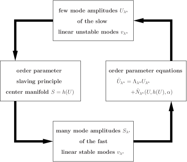
Figure 4: Circular causality chain of synergetics for the order parameter equations of the generalized Häussler equations (9). The control parameter $\alpha$ denotes the growth rate of new synapses onto the tectum.

paper we have proposed that the self-organized formation of retinotopic projections between manifolds of different geometries and dimensions is governed by a system of ordinary differential equations (9) which generalizes a former ansatz by Häussler and von der Malsburg Malsburg3 . The linear stability analysis determines the instability where an increase of the uniform growth rate $\alpha$ beyond the critical value (41) converts an initially disordered mapping into a retinotopic projection. Furthermore, it gives rise to a decomposition of the deviation from the stationary uniform solution $v(t,r)$ near the instability in unstable and stable contributions. By inserting this decomposition in the nonlinear Häussler equations (9), we obtain equations for the mode amplitudes of the unstable and stable modes, respectively. In the vicinity of the instability point the system generates a time-scale hierarchy, i.e. the stable modes evolve on a faster time-scale than the unstable modes. This leads to the slaving principle of synergetics: the stable modes are enslaved by the unstable modes. In the literature this enslaving $S=h(U)$ is usually achieved by invoking an adiabatic elimination of the stable modes, which amounts to solving the equation $\dot{S}=0$. However, the mathematically correct approach for determining the center manifold $h(U)$ is to determine it from the corresponding evolution equations for the stable modes wwp . It can be shown that only for real eigenvalues this approach leads to the same result obtained by the approximation $\dot{S}=0$. Thus, it is possible to reduce the original high-dimensional system to a low-dimensional one which only contains the unstable amplitudes. The general form of the resulting order parameter equations (86) is independent of the geometry of the problem. It contains typically a linear, a quadratic and a cubic term of the order parameters. As a general feature of synergetics, the coefficients (86), (88) consist of two parts, one stemming from the order parameters themselves and the other representing the influence of the center manifold on the order parameter dynamics.

Our results can be interpreted as an example for the validity of the circular causality chain of synergetics, which is illustrated in Figure 4. On the one hand, the order parameters, i.e. the few amplitudes $U_{\lambda^{u}}$ of the slowly evolving linear unstable modes $v_{\lambda^{u}}$, enslave the dynamics of the many stable mode amplitudes $S_{\lambda^{s}}$ of the fast evolving stable modes $v_{\lambda^{s}}$ through the center manifold. On the other hand, the center manifold of the stable amplitudes acts back on the order parameter equations.

VI Outlook

The order parameter equations (86)–(88) represent the central new result of this paper, and in the forthcoming publication gpw2 they will serve as the starting point to analyze in detail the self-organization in cell arrays of different geometries. To this end we assume that the manifolds are characterized by spatial homogeneity and isotropy, i.e. neither a point nor a direction is preferred to another, respectively. This additional assumption requires the manifolds to have a constant curvature and their metric turns out to be the stationary Robertson-Walker metric of general relativity Weinberg . We therefore have to discuss the three different cases where the curvature of the manifolds is positive, vanishes, or is negative. This corresponds to modelling retina and tectum by the sphere, the plane, or the pseudosphere.

A further intriguing problem concerns the question under what circumstances non-retinotopic modes become unstable and destroy the retinotopic order. One could imagine that some types of pathological development in animals corresponds to this case.

As already mentioned, lacking any theory for the cooperativity functions, we have regarded them as time-independent given properties of the manifolds. They are determined by the lateral connections between the cells of retina and tectum, respectively Malsburgskript . But neither a reason for their time-independence nor a detailed discussion of their precise mathematical form is available. To fill this gap it will be necessary to elaborate a self-consistent theory of the cooperativity functions.

Our generalized Häussler equations are fully deterministic. In real systems, however, there are always fluctuations. To take into account such unpredictable small variations a stochastic force has to be added to the deterministic part of the equation. Such fluctuations are known to play an important role, especially in the vicinity of instability points Risken ; Horsthemke .

Finally, delayed processes could be included in our considerations. Synergetic concepts have been successfully applied to time-delayed dynamical systems in Refs. wwp ; Grigorieva ; Simmendinger ; sp ; sp2 . In neurophysiological systems delays occur due to the finite propagation velocity of nerve signals bpw1 ; bpw2 as well as the finite duration of physiological processes such as the change of synaptic connection weights. Thus, it would be also worthwhile to expand the investigations to time-delayed Häussler equations.

References

- (1) E. R. Kandel, J. H. Schwartz, and T. M. Jessell (Eds.), Principles of Neural Science, fourth edition (McGraw-Hill, New York, 2000).
- (2) E. I. Knudsen and M. Konishi, Science 200, 795 (1978).
- (3) R. W. Sperry, J. Exper. Zool. 92, 263 (1943).
- (4) R. W. Sperry, J. Comp. Neurol. 79, 33 (1943).
- (5) R. W. Sperry, Proc. Natl. Acad. Sci. U.S.A. 50, 703 (1963).
- (6) G. J. Goodhill and L. J. Richards, Trends Neurosci. 22, 529 (1999).
- (7) C. von der Malsburg and D. J. Willshaw, Proc. Natl. Acad. Sci. U.S.A. 74, 5176 (1977).
- (8) D. J. Willshaw and C. von der Malsburg, Philos. Trans. R. Soc. London B 287, 203 (1979).
- (9) A. F. Häussler and C. von der Malsburg, J. Theoret. Neurobiol. 2, 47 (1983).
- (10) H. Haken, Synergetics – An Introduction, third edition (Springer, Berlin, 1983).
- (11) H. Haken, Advanced Synergetics (Springer, Berlin, 1983).
- (12) W. Wagner and C. von der Malsburg, private communication.
- (13) M. Güßmann, A. Pelster, and G. Wunner, A General Model for the Development of Retinotopic Projections Between Manifolds of Different Geometries; in R. P. Würtz and M. Lappe (Editors), Proceedings of the 4. Workshop Dynamic Perception, Bochum, Germany, November 14-15, 2002; Akademische Verlagsgesellschaft Berlin, p. 253 (2002).
- (14) G. J. Goodhill and J. Xu, Network 16, 5 (2005).
- (15) N. V. Swindale, Network 7, 161 (1996).
-
(16)
M. Güßmann, Self-Organization between Manifolds of Euclidean and non-Euclidean
Geometry by Cooperation and Competition, Ph.D. Thesis (in german), Universität Stuttgart (2006);
internet: www.itp1.uni-stuttgart.de/publikationen/guessmann_doktor_2006.pdf. - (17) W. Wischert, A. Wunderlin, A. Pelster, M. Olivier, and J. Groslambert, Phys. Rev. E, 49, 203 (1994).
- (18) M. Güßmann, A. Pelster, and G. Wunner, Ann. Phys. (Leipzig) 16, 395 (2007)
- (19) S. Weinberg, Gravitation and Cosmology – Principles and Applications of the General Theory of Relativity (John Wiley & Sons, New York, 1972).
-
(20)
C. von der Malsburg, Neural Network Self-organization (I) – Self-organization in the Development of the Visual System. Lecture Notes (2000);
internet: www.neuroinformatik.ruhr-uni-bochum.de/VDM/
exercises/ALL/SS/courses/summer.pdf. - (21) H. Risken, The Fokker-Planck Equation. Methods of Solution and Applications, second edition (Springer, Berlin, 1989).
- (22) W. Horsthemke and R. Lefever, Noise-Induced Transitions (Springer, New York, 1984).
- (23) E. Grigorieva, H. Haken, S.A. Kashchenko, and A. Pelster, Physica D 125, 123 (1999)
- (24) C. Simmendinger, A. Pelster, and A. Wunderlin, Phys. Rev. E 59, 5344 (1999)
- (25) M. Schanz and A. Pelster, Phys. Rev. E 67, 056205 (2003).
- (26) M. Schanz and A. Pelster, SIAM Journ. Appl. Dyn. Syst. 2, 277 (2003).
- (27) S. F. Brandt, A. Pelster, and R. Wessel, Phys. Rev. E 74, 036201 (2006).
- (28) S. F. Brandt, A. Pelster, and R. Wessel, eprint: physics 0701225.